2019
Enhancing the performance of energy harvesting
wireless communications using optimization and
machine learning
Ala'eddin A. Masadeh
Iowa State University
Follow this and additional works at:
https://lib.dr.iastate.edu/etd
Part of the
Computer Engineering Commons, and the
Electrical and Electronics Commons
This Dissertation is brought to you for free and open access by the Iowa State University Capstones, Theses and Dissertations at Iowa State University Digital Repository. It has been accepted for inclusion in Graduate Theses and Dissertations by an authorized administrator of Iowa State University Digital Repository. For more information, please [email protected].
Recommended Citation
Masadeh, Ala'eddin A., "Enhancing the performance of energy harvesting wireless communications using optimization and machine learning" (2019).Graduate Theses and Dissertations. 17263.
optimization and machine learning
by
Ala’eddin Masadeh
A dissertation submitted to the graduate faculty in partial fulfillment of the requirements for the degree of
DOCTOR OF PHILOSOPHY
Co-majors: Electrical Engineering; Computer Engineering Program of Study Committee:
Ahmed E. Kamal, Co-major Professor Zhengdao Wang, Co-major Professor
Daji Qiao Lu Ruan Sang W. Kim
The student author, whose presentation of the scholarship herein was approved by the program of study committee, is solely responsible for the content of this dissertation. The
Graduate College will ensure this dissertation is globally accessible and will not permit alterations after a degree is conferred.
Iowa State University Ames, Iowa
2019
DEDICATION
I would like to dedicate this thesis to my family, especially to my extraordinary parents. All of this was, is and always will be for them.
TABLE OF CONTENTS
CHAPTER LIST OF FIGURES . . . vi
LIST OF ABBREVIATIONS . . . viii
LIST OF SYMBOLS . . . x
ACKNOWLEDGEMENTS . . . xiii
ABSTRACT . . . xiv
CHAPTER 1. INTRODUCTION . . . 1
1.1 Background . . . 1
1.1.1 Energy Harvesting Wireless Devices . . . 2
1.1.2 Cognitive Radio . . . 2
1.1.3 Cooperative Relaying . . . 3
1.2 Related Works . . . 4
1.2.1 Energy Harvesting Cognitive Radio with Cooperative Communications . 4 1.2.2 Energy Harvesting Communications with Non-Causal Knowledge . . . . 5
1.2.3 Energy Harvesting Communications with Statistical Knowledge . . . 6
1.2.4 Energy Harvesting Communications in Unknown Environments . . . 7
1.2.5 Exploration and Exploitation in Reinforcement Learning . . . 8
1.2.6 Model-free and Model-based Reinforcement Learning . . . 9
1.2.7 Off-policy Reinforcement Learning . . . 11
1.3 Thesis Scope and Contributions . . . 12
1.4 Thesis Organization . . . 15
CHAPTER 2. MARKOV DECISION PROCESS AND REINFORCEMENT LEARNING 16 2.1 Markov Decision Process . . . 16
2.2 Problem Formulation of Decision Making in Uncertain Environments . . . 18
2.3 Value Functions . . . 18
2.4 Reinforcement Learning . . . 19
CHAPTER 3. COGNITIVE RADIO NETWORKING WITH ENERGY HARVESTING AND COOPERATIVE RELAYING . . . 22
3.1 System Model . . . 22
3.2 Problem Formulation . . . 24
3.3 Proposed Solution . . . 27
3.4 Simulation Results . . . 31
CHAPTER 4. LOOK-AHEAD AND LEARNING APPROACHES FOR ENERGY
HARVESTING COMMUNICATIONS SYSTEMS . . . 35
4.1 System Model . . . 36
4.2 Problem Formulation . . . 37
4.2.1 Throughput Maximization Problem . . . 37
4.2.2 MDP Reformulation . . . 39
4.3 Look-ahead Policy for EH Communications (known underlying model) . . . 40
4.3.1 Two-step look-ahead throughput . . . 41
4.3.2 Look-ahead throughput algorithm . . . 41
4.4 RL for EH Communications (unknown underlying model) . . . 42
4.4.1 RL prediction methods . . . 42
4.4.2 RL exploration algorithms . . . 43
4.5 Complexity . . . 47
4.6 Simulation Results . . . 47
4.6.1 Comparison with the upper bound . . . 49
4.6.2 Comparison in large scenario . . . 50
4.6.3 RL algorithms - harvested energy levels with equal probabilities . . . . 52
4.6.4 Effect of theτ in Convergence-based algorithm . . . 52
4.6.5 Effect of theζ in Convergence-based algorithm . . . 53
4.6.6 Effect of the in-greedy algorithm . . . 54
4.7 Chapter Summary . . . 55
CHAPTER 5. REINFORCEMENT LEARNING ARCHITECTURES . . . 57
5.1 The Estimator-Selector-Actor-Critic Architecture . . . 58
5.1.1 Actor-Critic . . . 58
5.1.2 Selector-Actor-Critic . . . 60
5.1.3 Tuner-Actor-Critic . . . 61
5.1.4 Estimator-Selector-Actor-Critic . . . 63
5.1.5 Discussions . . . 65
5.2 Energy Harvesting Communications Supported by Reinforcement Learning Architectures . . . 66
5.2.1 System Model and Problem Formulation . . . 66
5.2.2 EH Communications System Supported by RL Architectures . . . 66
5.2.3 Exponential Softmax Policy . . . 68
5.2.4 Experimental Results . . . 69
5.3 Chapter Summary . . . 76
CHAPTER 6. AN ACTOR-CRITIC REINFORCEMENT LEARNING APPROACH FOR ENERGY HARVESTING COMMUNICATIONS SYSTEMS . . . 78
6.1 System Model . . . 78 6.2 Problem Formulation . . . 79 6.3 Actor-Critic . . . 81 6.3.1 Actor . . . 81 6.3.2 Critic . . . 83 6.4 Simulation Results . . . 83
6.4.1 The cumulative discounted return for actor-critic versus hasty . . . 84
6.4.2 The effect of the approximated value function on the cumulative discounted return . . . 85
CHAPTER 7. CONCLUSIONS AND FUTURE WORK . . . 87
7.1 Conclusions and Contributions . . . 87
7.2 Future Work . . . 90
LIST OF FIGURES
Figure 2.1 The agent-environment interaction in MDP. . . 16
Figure 2.2 Markov decision process. . . 17
Figure 3.1 Cooperative underlay CR system with EH. . . 23
Figure 3.2 Slotted system model for EH nodes. . . 24
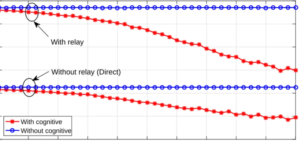
Figure 3.3 Secondary sum rate of direct and relayed transmission systems with and without CR versus primary SINR. . . 32
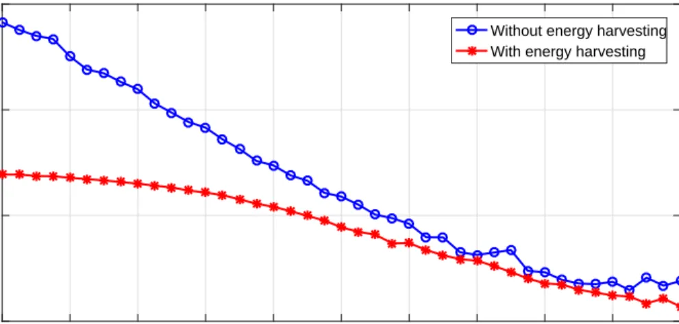
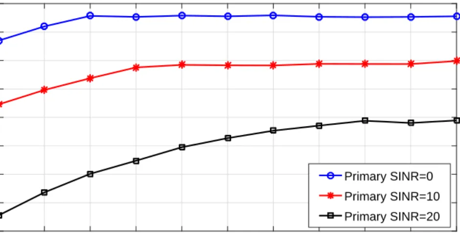
Figure 3.4 Sum rate from the SR to the SD with and without EH versus different values for SINR at the primary network. . . 33
Figure 3.5 The effect of increasing the extra time on sum rate the SR to the SD versus number of extra time slots. . . 34
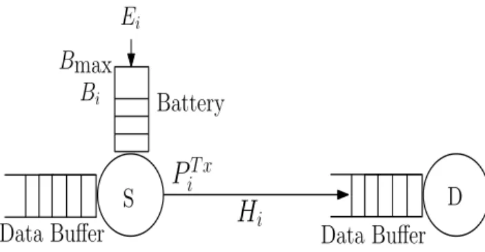
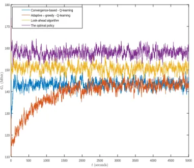
Figure 4.1 Point-to-point communication system with an energy harvesting source. 36 Figure 4.2 The discounted returnGt versus timet for different approaches. . . 50
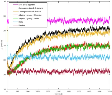
Figure 4.3 The discounted returnGt versus timet for different approaches. . . 51
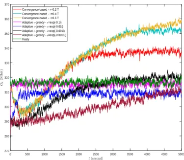
Figure 4.4 The discounted return Gt versus time t for different RL exploration algorithms. . . 53
Figure 4.5 The discounted returnGt versus timet for different values of theτ. . . 54
Figure 4.6 The discounted returnGt versus timet for different values of theζ. . . 55
Figure 4.7 The discounted returnGt versus timet for different values of the. . . 56
Figure 5.1 Actor-critic architecture. . . 59
Figure 5.2 Selector-actor-critic architecture. . . 61
Figure 5.3 Tuner-actor-critic architecture. . . 62
Figure 5.4 Estimator-selector-actor-critic architecture. . . 64
Figure 5.5 The cumulative discounted returnGt versust. . . 71
Figure 5.6 The total rewardsG0 versusT. . . 72
Figure 5.7 The cumulative discounted returnGt versustwhen γ = 0.9. . . 73
Figure 5.8 The total rewardsG0 versusT when γ = 0.9. . . 73
Figure 5.9 The returnGt versust when γ= 0.0. . . 74
Figure 5.10 The fitted returnGt versustwhen γ = 0.0. . . 75
Figure 5.11 The average returnGt(w) versustwhen γ = 1.0. . . 75
Figure 5.12 The average rewardG0(w) versuswwhen γ = 1.0. . . 76
Figure 6.2 The cumulative discounted returnGt versus t. . . 84
LIST OF ABBREVIATIONS
AC Actor-Critic
AF Amplify and Forward
AI Artificial Intelligence
CR Cognitive radio
CRN Cognitive Radio Network
CSI Channel State Information
DF Decode and Forward
DP Dynamic Programming
EH Energy Harvesting
EnHANTs Energy-Harvesting Active Networked Tags
ESAC Estimator-Selector-Actor-Critic
FCC Federal Communications Commission
i.i.d Independent and Identically Distributed
MDP Markov Decision Process
MLAC Model Learning Actor-Critic
RMAC Reference Model Actor-Critic
MPI Modified Policy Iteration
PAMDP Parameterized Action Space Markov Decision Processes
PI Policy Iteration Algorithm
QoS Quality of Service
RF Radio Frequency
RL Reinforcement Learning
SAC Selector-Actor-Critic
SINR Signal-to-Interference-plus-Noise Ratio
TAC Tuner-Actor-Critic
TD Temporal-Difference
LIST OF SYMBOLS
Bmax The maximum capacity of a battery
Bi Battery level at time sloti
Bx,i Battery level of node x at time sloti
PT xi Transmission power during time slot i
PT xx,i Transmission power by node x during time sloti
Ei Harvested energy during time sloti
Ex,i Harvested energy by node x during theith time slot
d(x,y) Distance between node x and node y
Hi The channel signal gain at time sloti
H(x,y),i Channel signal gain between the nodes x and y during time slot i
˜
H(x,y),i The fading coefficient between x and y during time slot i
αpl Path loss exponent
yx,i The received signal at node x during the time sloti
xx,i The transmitted signal from node x during the time sloti
nx,i The additive Gaussian noise at node x during time sloti
σn2 The noise variance
σn,i2 The noise variance during time slot i
σ The standard deviation of the normal distribution
µ The mean of the normal distribution
Γx,i The SINR at node x during time sloti
Γ The predefined SINR QoS threshold
log(·) Logarithm function
| · | Absolute value of a function or cardinality of a set
B Bandwidth
i Time step number
T Final time step of an episode
S Set of possible states
A Set of possible actions
Si The state at time sloti
Ai The taken action at time sloti
s A state
a An action
ag The greedy action at states, i.e., ag = argmax
b
Q(s, b), ∀bats
al Thelth action
sj Thejth state
A(s) The set of actions available at states
Ns The total number of all possible states
Na The total number of available actions
π(s) Action taken in state sunder deterministic policy π
π(a|s,θ) Probability selecting actionaat statesgiven parameter vectorθ
θ Parameter vector of target policy
w Vector of weights used to approximate value function
π∗ The optimal policy
J(θ) Performance measure for policy π(a|s,θ)
dπ(s) The steady-state distribution of the underlying MDP using policyπ
E[Z] Expectation of a random variableZ
Pr(Z =z) Probability that a random variableZ takes a value ofz
p(s0|s, a) Probability of transition from states to states0 under action a
r(s, a, s0) The expected reward for state-action-next-state
Ri Reward at timei
vπ∗(s) State-value ofsunder the optimal policy
qπ(s, a) Action-value of state-action pair (s, a) under policyπ
qπ∗(s, a) Action-value of state-action pair (s, a) under the optimal policy
V Estimate of state-value functionvπ
Q Estimate of action-value functionqπ
φ(s) vector of features at states
φ(s, a) vector of features for (s, a) state-action pair
u Random disturbance
γ Discount factor
α, β Step-size parameters
ζ The action-value function convergence error in the convergence-based
exploration algorithm
τ The exploration time threshold in the convergence-based exploration algorithm
Probability of random action in-greedy policy
B The set of battery levels
bj Thejth battery level
NB Number of possible battery levels
En The set of energy levels that can be harvested
ej Thejth level of energy that can be harvested
Ne Number of energy levels that can be harvested
pEn(e
0|e) The transition probability from harvested energy leveleto levele0
H The set of channel gains
hj Thejth channel gain
NH Number of possible channel gains
pH(h0|h) The transition probability from channel gainh to channel gainh0
PT x The set of transmission power levels
pT xj Thejth power level that can be transmitted
ACKNOWLEDGEMENTS
“After all this time”... “Always”.
Firstly, I thank Allah for allowing me to reach this milestone. This journey would have been meaningless without him. He has been my source of strength all throughout. I thank Allah for the extraordinary parents he has given me. I am nothing without them. Secondly, I thank my wonderful major advisers Professor Ahmed E. Kamal and Professor Zhengdao Wang for their support, patience, and guidance in almost every step throughout my thesis. And finally, I thank my friends I have made along the way. They have left wonderful memories for me.
ABSTRACT
The motivation behind this thesis is to provide efficient solutions for energy harvesting
communications. Firstly, an energy harvesting underlay cognitive radio relaying network
is investigated. In this context, the secondary network is an energy harvesting network.
Closed-form expressions are derived for transmission power of secondary source and relay that maximizes the secondary network throughput. Secondly, a practical scenario in terms of information availability about the environment is investigated. We consider a communications system with a source capable of harvesting solar energy. Two cases are considered based on the knowledge availability about the underlying processes. When this knowledge is available, an algorithm using this knowledge is designed to maximize the expected throughput, while reducing the complexity of traditional methods. For the second case, when the knowledge
about the underlying processes is unavailable, reinforcement learning is used. Thirdly, a
number of learning architectures for reinforcement learning are introduced. They are called
selector-actor-critic, tuner-actor-critic, and estimator-selector-actor-critic. The goal of the
selector-actor-critic architecture is to increase the speed of learning a suboptimal policy by approximating the most promising action at the current state. The tuner-actor-critic aims at improving the learning process by providing the actor with a more accurate estimation about the value function. Estimator-selector-actor-critic is introduced to support intelligent agents. This architecture mimics rational humans in the way of analyzing available information, and making decisions. Then, a harvesting communications system working in an unknown environment is evaluated when it is supported by the proposed architectures. Fourthly, a realistic energy harvesting communications system is investigated. The state and action spaces of the underlying Markov decision process are continuous. Actor-critic is used to optimize the system performance. The critic uses a neural network to approximate the action-value function. The actor uses policy gradient to optimize the policy’s parameters to maximize the throughput.
CHAPTER 1. INTRODUCTION
1.1 Background
Energy harvesting (EH) technology has been considered as an efficient solution that provides sustainable wireless communication systems. EH communications have been introduced to develop communication devices that are able to recharge their batteries using natural sources, and then use this energy for data transmission [1]. The lifetimes of EH devices are determined by their hardware lifetimes, since they are able to recharge their batteries. In addition, the possibility of deploying these devices in hard-to-reach places [2].
To implement efficient EH communications networks, it is important to consider two objectives, which are prolonging the network’s lifetime and maximizing its throughput. This can be achieved by optimizing and managing the networks’ resources especially in unknown environments [3].
Managing the use of the harvested energy for data transmission is the main challenge facing EH communications [3]. This is because of changing the amount of energy that can be harvested over time [1]. To overcome this challenge and to improve the performance of such systems, it is important to design power allocation policies that consider time-variant EH and the channel fading processes.
The issue of designing power allocation policies for data transmission based on the available information at the EH nodes has been investigated. This available knowledge at EH nodes can be classified into three groups. The first one is the non-causal knowledge. In this case, it is assumed that the EH nodes have perfect non-causal knowledge about the EH and the channel fading processes. This assumption insures an optimal allocation policy. The second group is the statistical knowledge, where the EH and the channel fading processes are stationary random
processes. The last group is the causal knowledge, which is the most realistic one. This means that at every time slot, EH nodes have only current and past information about harvested energy and channel gains [3].
Considering the most realistic scenario introduces a challenge in designing power allocation policies for EH networks. This challenge is to balance energy saving and energy consumption in unknown environments [3]. One of the promising methods to design allocation policies in such environments is reinforcement learning (RL). RL is known as a learning technique to know what to do in an unknown environment in order to maximize a numerical return [4].
1.1.1 Energy Harvesting Wireless Devices
Recently, EH has been considered as one of the promising solutions for sustainable wireless communications. EH technology converts the ambient energy into usable electric energy [5]. Current EH techniques are able to provide limited levels of energy, e.g., an outdoor solar panel
can get the benefit of 10 mW/cm2 solar energy flux with harvesting efficiency taking values
between 5% and 30%, depending on the used material [6].
EH wireless devices are characterized by a number of properties, which make them attractive to a number of applications. One of these properties is their ability to provide communications in hard-to-reach or inaccessible areas, where replenishing batteries or recharging them is difficult. In addition, these devices have lifetimes that are limited by the lifetimes of their hardware [2]. Last but not least, They provide green or environment friendly devices that preserve the environment by reducing the pollution [7].
For EH wireless nodes, there are five types of energy that can be converted to electrical energy to power this type of nodes. These types are vibration, ambient light, radio frequency (RF) waves, temperature difference, and human body energy [8].
1.1.2 Cognitive Radio
Demands on wireless services have been increasing, which yields to what is known as spectrum congestion. Spectrum congestion can be defined as the spectrum scarcity, which makes it difficult to accommodate a number of wireless devices at the same time [9].
A number of recent studies have shown that the actual utilization of the licensed spectrum band varies from 15% to 85%, which motivated the Federal Communications Commission (FCC) to propose opportunistic utilization of the licensed band to overcome the spectrum shortage problem [9].
Cognitive radio (CR) can be defined as the technology that enables secondary users to utilize the primary spectrum (i.e. the licensed spectrum) opportunistically. The importance of this technology comes from the possibility of improving the spectrum utilization in a way that allows the next generation mobile devices to utilize the available spectrum efficiently [10].
There are three operating modes for cognitive radio networks (CRN), which are underlay, overlay or interweave [11; 12]. In a CR underlay setup, both primary and secondary users access the spectrum simultaneously. In order to protect the primary Quality-of-Service (QoS), the interference from all secondary nodes should be kept under a certain tolerance limit [13]. The overlay mode is based on cooperation between secondary and primary users. For instance, the secondary user relays the primary user’s signal in order to get an opportunity to transmit its data using the primary spectrum [14]. In the interweave mode, the secondary users are allowed to utilize the primary spectrum holes opportunistically when they are unoccupied by the licensed users. In this mode, there is a crucial process that should be taken before utilizing the primary spectrum by the secondary users, which is the spectrum sensing [14]. It is reported by a number of works that imperfect sensing may result in degrading the network performance [15; 16].
1.1.3 Cooperative Relaying
Cooperative communication is characterized by a number of properties that make it an efficient technology in wireless communications. Some of the main properties of this technology can be summarized as its ability to improve the capacity, reduce the transmission powers, extend the coverage area, and combat fading of wireless channels [17; 18].
Using this technology, relay(s) are used to forward data from the source to the destination
[17]. For this technology, there is a number of protocols to implement cooperative
protocols, there are two well-known protocols, which are amplify and forward (AF) and decode and forward (DF). In AF, a relay amplifies received signals from the source, and then, transmits them to the destination. On the other hand, in DF relaying, a relay is used to decode the received signal firstly, and then, it re-encodes and transmits the signal to the destination [17].
1.2 Related Works
Before going into the details of our proposed models, some recent related works are reviewed in this chapter.
1.2.1 Energy Harvesting Cognitive Radio with Cooperative Communications Energy Harvesting Cooperative Communications. Recently, EH has been considered as one of the promising solutions for sustainable wireless communications. Energy harvesting technology converts the ambient energy into usable electric energy [5]. Current EH techniques are able to provide limited levels of energy, e.g., an outdoor solar panel can get the benefit of
10 mW/cm2 solar energy flux with harvesting efficiency taking values between 5% and 30%,
depending on the used material [6]. At the same time, cooperative communication is one of the advanced technologies in wireless communications [20; 19], where the wireless nodes assist each other in delivering their data in order to achieve more reliable communication [21]. Combining EH with cooperative relaying can further achieve energy efficient reliable communication, in [22] the authors examined EH with cooperative communication system and energy transfer property. They assume that both source and relay can harvest energy from ambient environment. In addition, the relay can harvest energy RF signals from the source. The framework objective is to maximize the end-to-end throughput by optimizing transmission powers and energy transfer.
Energy Harvesting Cognitive Radio Networks. Combining EH with CR aims to allocate the spectrum efficiently in a green manner [23; 24; 25; 26]. In a CR underlay setup, both primary and secondary users access the spectrum simultaneously. In order to protect the primary Quality-of-Service (QoS), the interference from all secondary nodes should be kept
under a certain tolerance limit [27]. For instance, the authors in [13] study the EH underlay CRN with cooperation between the secondary and the primary users, where the secondary user, who shares the spectrum owned by the primary, is equipped with EH capability and has finite capacity battery for energy storing. In return, the secondary user transfers portion of its energy to the primary user.
Energy Harvesting Cognitive Radio Networks with Cooperative Relaying.
Moreover, cooperative communication can be used in EH-CR networks in order to enhance the system performance, where the performance of the EH-CR combined with cooperative relay outperforms the performance of the direct link communication (i.e., without relays) specially if the distance between the communication terminals is relatively large, the available energy is limited, and the interference constraint is very low.
Combining these three technologies has been investigated [28; 29]. For instance, the authors in [28] studied a cooperative EH with a cognitive overlay system, in which the secondary user utilizes portion of the primary time for its transmission data. In return, acting as a relay for the primary user, the secondary user can help in primary transmission. In their proposed model, two RF EH techniques were used at the relay side. In [29], the authors investigated the problem of observing the secondary users sequentially to be used as cooperative relay to the primary transmitter. They derived an optimal stopping rule that selects a relay from a set of candidates to help in relay transmission, which maximizes the observation efficiency.
1.2.2 Energy Harvesting Communications with Non-Causal Knowledge
EH communications systems with non-causal knowledge have been widely discussed [30; 31; 32; 33; 34; 35]. Management approaches in this case are called offline approaches, where the amounts of harvested energy and their arrival times are known at the beginning of the communication session [36]. Despite the difficulty of considering this assumption in reality, it is used to find the upper bound performance [30].
In [30], the problem of maximizing the throughput of EH single hop communication system with non-causal knowledge is investigated. The authors prove that this problem can be modeled
as the minimization of the time required for transmitting a fixed amount of data. The problem of identifying the offline transmission policy for EH communications system with cooperative relay is discussed in [31]. The goal is to maximize the amount of data received by the destination within a given time interval. In the proposed model, both the transmitter and the relay are EH nodes. The model is investigated under two scenarios, which are half-duplex and full-duplex relaying for communications. In [35], the problem of finding the offline transmission power allocation for EH communications system with multiple half-duplex relays is studied. The problem is formulated as a convex optimization problem to find the optimal power allocation for the goal of maximizing the amount of delivered data by a deadline.
1.2.3 Energy Harvesting Communications with Statistical Knowledge
For modeling more realistic EH communications systems, it is assumed that the EH, and data generation processes are discrete Markov processes with full statistical knowledge [37; 38; 39]. A Markov decision process (MDP) is characterized by its ability to provide a suitable mathematical framework for modeling decision-making problems when the system has processes that follow the Markov property [38]. Due to its efficiency, MDP has been adopted to deal with a number of problems considering EH [37; 38; 39; 40]. In [38], a point-to-point wireless communication system is studied, where the transmitter is able to harvest energy and store it in a rechargeable battery. The goal is to maximize the expected total transmitted data during the activation time of the transmitter. The problem is formulated as a discounted MDP problem. The state space consists of the battery state, the size of the packet to be transmitted, the current channel state, and the amount of energy needed for transmitting this packet successfully. At the beginning of each time slot, the transmitter makes a binary decision, whether to drop or to transmit the packet based on the current conditions. In this work, policy iteration (PI) is employed to solve the problem. In [40], an CRN with a secondary user that is capable of harvesting RF energy is investigated. In this model, the secondary user cannot execute EH and data transmission simultaneously, since it has only one interface. As a result, at the beginning of each time slot, the secondary user has to select either harvesting or transmitting. The mode management problem is formulated as an MDP. The primary channel is modeled
as a three-state Markov chain, these states are occupied, idle with bad quality, and idle with good quality. The state space of the modeled MDP is a combination of the primary channel states and the secondary user energy levels. The action space consists of two actions, which are to harvest or to transmit. Value iteration (VI) is used to find the optimal policy, and the performance is compared with the greedy policy.
While traditional methods such as VI are able to find the optimal policy for MDP problems [41; 42], the complexity to find optimal solution grows as the number of states and actions
increases. The complexity of finding the optimal solution using VI is O(|A|.|S|2), where A
is the set of actions, S is the set of states for the problem [43]. This has encouraged finding
alternative methods for solving MDP problems, especially in the case of having large numbers of states and actions [37; 40; 44; 45]. The authors in [37] consider a network of objects equipped with energy-harvesting active networked tags (EnHANTs). The goal is to design an optimal transmission strategy for the EnHANTs to adapt to changes in the amounts of harvested energy and the identification request. The problem is formulated as an MDP. Modified policy iteration (MPI) method [46] is employed to solve the problem and to overcome the complixity of exhaustive search. In [45], the idea of using a mobile energy gateway is investigated, which has the capability of receiving energy from a fixed charging facility, as well as transferring energy to other users. The goal is to maximize the utility by taking the optimal action of energy charging/transferring. The problem is formulated as an MDP. The authors prove that there is a threshold structure of the optimal policy with respect to the system states, which helps in obtaining the optimal policy especially for MDPs with large numbers of states. The goal of determining these thresholds is to select immediate optimal actions based on the current state instead of using the traditional methods such as VI.
1.2.4 Energy Harvesting Communications in Unknown Environments
In the previous two frameworks, a priori knowledge, either deterministic or statistical, about the EH process is required. However, this knowledge might be unavailable, in which case reinforcement learning (RL) can be used to improve the performance of such systems [36]. RL enables an autonomous agent to optimize its policy in an unknown environment [4; 47].
In [3; 36], the problem of optimizing EH communications systems is investigated using RL. In this context, at any time, the EH nodes have only current local knowledge of the EH process. The authors aim to find a power allocation policy that maximizes the throughput. In these two works, the RL algorithm, which is known as the state-action-reward-state-action (SARSA), is
used to evaluate the taken actions. On the other hand, the -greedy exploration algorithm is
used to balance between exploring and exploiting available actions.
In [38], a point-to-point communications system is investigated. The transmitter is capable of harvesting energy and storing it in a rechargeable battery. The energy and data arrivals are formulated as Markov processes. In this work, the authors use Q-learning to find the optimal transmission policy when the system does not have a priori information about the
Markov processes governing the system. They use the-greedy exploration algorithm to balance
between exploration and exploitation.
1.2.5 Exploration and Exploitation in Reinforcement Learning
RL enables an autonomous agent to optimize its policy to maximize its total expected reward. Here, the agent is placed in an unknown environment, and learns by trial and error [48].
A deterministic policy π can be defined as a function specifying the action π(s) that is
taken by the agent when it is in states. At any time, there is at least one action for each state
that has highest estimated value, this action is called a greedy action. If the greedy action is selected, this mode is called exploitation, where the agent exploits its current knowledge to determine the current best action (i.e. greedy action), and then use it. On the other hand, when a nongreedy action is selected, this mode is called exploration. Exploration enables the agent to improve its estimates about the nongreedy actions, and discover which of them has higher value than the greedy action [4].
Exploitation should be used when the available time is limited, in which exploring new actions may degrade the performance. If this short time is used for exploration, it may result in exploring unfavorable actions, hence wasting the opportunity of exploiting a current greedy action. Meanwhile, when the available time is abundant and there is ample time to explore
all available actions, then exploration may result in discovering better actions, and exploit them in the remaining time. Balancing between exploration and exploitation is a crucial factor that affects the cumulative rewards. This introduces the importance of balancing between exploration and exploitation, which is one of the main challenges that face RL, and is known as the exploration-exploitation dilemma [4; 49].
Boltzmann and -greedy exploration algorithms are considered as the most popular
exploration algorithms [50], where they are intensively used in the literature [49; 51; 52; 53; 54; 55; 47]. These methods depend on random action selection to learn about new actions [50]. In
-greedy, the agent selects a new action from uniformly distributed actions with probability,
while the greedy action is selected with probability 1− [53]. On the other hand, Boltzmann
or softmax exploration uses Boltzmann distribution to assign selection probability to actions [49].
Developing new and efficient exploration algorithms is an active area of research [56], where the goal is to enhance RL algorithms, and make them applicable for real applications. Due to these reasons, this topic has been widely investigated [56; 57; 58]. In [56], a counting-based
exploration algorithm is designed. The count for state-action visitation count(s, a) is added
to the Boltzmann equation to control the exploration. Each time an action a at state s is
selected, the count(s, a) increases by one. The main idea of adding this parameter is for
balancing between exploration and exploitation and improving the performance.
In [57], the authors proposed the idea of adapting existing exploration algorithms, and combining them with each other. This work studies structured parameterized action space Markov decision processes (PAMDP), where there is a set of discrete actions, each action is parameterized with continuous parameters. For the goal of addressing the exploration of both discrete actions and the continuous parameters, it is proposed to use Boltzmann equation for discrete exploration, and Gaussian exploration to explore the continuous parameters.
1.2.6 Model-free and Model-based Reinforcement Learning
RL methods are categorized into two classes, which are model-free learning and model-based learning. Model-free learning updates the value function after interacting with an environment
without learning the underlying model. On the other hand, model-based learning estimates the dynamics of an environment firstly, and then, dynamic programming (DP) is used to optimize the policy [59; 60].
Each learning class has its own advantages, and suffers from a number of weaknesses. Model-based learning is characterized by its efficiency in learning [61], but at the same time,
it struggles in complex problems [62]. On the other hand, model-free learning has strong
convergence guarantees under certain situations [4], but the value functions change slowly over time [63], especially, when the learning rate is small.
Merging methods from the two learning classes aims at implementing intelligent agents, and to overcome the mutual weaknesses of these two classes. Combining methods from both learning classes has been discussed in many works [64; 65; 66; 67; 68; 69; 70]. In [64], a method called model-guided exploration was presented. This method integrated a learned model into an off-policy learning such as the Q-learning. The learned model is used to generate good trajectories using trajectory optimization, and then, these trajectories are mixed with on-policy experience to learn the agent. The improvement of this method is quite small even when the learned model is the true model. This returns to the reason of using two completely different policies for learning. This also can be explained by the need to learn bad actions too, so that the agent can distinguish between bad and good actions.
To overcome the weaknesses of the model-guided exploration algorithm, another algorithm called imagination rollout was designed [64]. It was proposed for applications that need large amounts of experience, or when undesirable actions are expensive. In this approach, synthetic samples are generated from the learned model that are called the imagination rollouts. These rollouts, the on-policy samples, and the optimized trajectories from the learned model are used with various mixing coefficients to evaluate each experiment. In each experiment, additional on-policy synthetic rollouts are generated from each visited state, and the model is refitted.
In [66], an algorithm called approximate model-assisted neural fitted Q-iteration was proposed. Using this algorithm, virtual trajectories are generated from a learned model to be used for updating the Q function. This work mainly aimed at reducing the amount of real trajectories required to learn a good policy.
Actor-critic (AC) is a model-free RL method, where the actor learns the policy that is modeled by a parameterized distribution, and the critic learns the value function. The actor optimizes the policy’s parameters to maximize the return, while the critic evaluates the performance of the policy. In [65], the framework of human-machine nonverbal communication was discussed. The goal was to enable machines to understand people intention from their behavior. AC with model-based learning were used. The learned dynamics of the underlying model are used to control over the temporal difference error (TD), and the actor uses the TD to optimize the policy for exploring different actions.
In [67], two learning algorithms were designed. The first one is called model learning
actor-critic (MLAC), while the second one is called reference model actor-critic (RMAC). The MLAC is an algorithm that combines AC with model-based learning. In this algorithm, the
gradient of the approximated state-value function ˆV(s) with respect to the state s, and the
gradient of the approximated model s0 = f(s, a) with respect to the action a are calculated.
The actor is updated by calculating the gradient of ˆV(s) with respect toausing the chain rule
and the previously mentioned two gradients. However, using RMAC, two functions are learned.
The first function is the underlying model. The second one is the reference model s0 =R(s),
which maps statesto the desired next states0 with the highest possible value. Then, using the
inverse of the approximated underlying model, the desired action can be found. The integrated paradigm of the reference model and the approximated underlying model serves as an actor, which maps states to actions.
1.2.7 Off-policy Reinforcement Learning
One of the promising methods for developing data efficient RL is off-policy RL. It does not learn from the policy being followed like on-policy methods, it utilizes and learns from data generated from past interactions with the environment [71]. Off-policy learning has been investigated in many works [71; 72; 73; 74].
Q-learning is considered as the most well known off-policy RL method [72]. It enables agents to act optimally in Markovian environments. This method evaluates an action at a state using its current value, the received immediate reward resulting from this action, and the value of the
expected best action at the next state. This expected best action at the next state is selected independently of the currently executed policy, which is the reason for classifying this method as an off-policy learning method.
Combining off-policy learning with AC was studied in [73]. As mentioned, it is the first AC algorithm that can be applied off-policy, where a target policy is learned while following and getting data from another behavior policy. A stream of data (a sequence of states, rewards, and actions) is generated according to a fixed behavior policy. Using this algorithm, the critic learns off-policy estimates of the value function. Then, these estimates are used by the actor for updating the weights of the target policy, and so on.
Using off-policy data to estimate the policy gradient accurately for a target policy was
investigated in [71]. A method called behavior policy gradient [75] is used to generate a
behavior policy with low variance estimates from a target policy. Trajectories generated from the behavior policy are used to estimate the direction of the policy gradient of the target policy.
1.3 Thesis Scope and Contributions
The thesis aims at providing energy efficient planning for wireless communications and developing algorithms to achieve this goal. The main contributions are summarized as follows:
1. In Chapter 3, the problem of optimizing the transmission power for underlay CR
networking with cooperative relaying and EH is investigated. The contributions can
be summarized as follows:
• Formulating an offline optimization problem aims at maximizing the sum rate of EH
source and relay in the secondary network while satisfying the primary QoS.
• The optimization problem is a non-convex problem. The problem is transformed to
an equivalent convex form using change of variables.
• The projected subgradient method is used to find the power allocated to the
secondary network.
• Finally, comparisons are made between the proposed system and other conventional
2. Chapter 4 investigates the performance of a point-to-point EH communications system in uncertain environments. Two scenarios are considered. The first one assumes that the EH node has only statistical knowledge about the harvested energy and channel gains. In the second scenario, the EH node works in an unknown environment. The contributions of this chapter can be summarized as follows
• The decision making problem for the considered EH communications is formulated
as an optimization problem.
• Due to the unavailability of non-causal knowledge about the channel gain and energy
arrival processes, the problem is reformulated as a discrete state and action MDP.
• An algorithm was designed to find a suboptimal power allocation policy when the
statistical knowledge about the environment is available. This algorithm is called “Look-ahead Algorithm for EH Communications”.
• RL is used when the EH nodes have only causal knowledge about the environment.
• A new exploration algorithm for RL called “convergence-based algorithm” is
introduced.
• The introduced algorithms were evaluated by comparing their performance with
other algorithms.
3. In Chapter 5, a number of proposed architectures for RL are presented. These
architectures are called tuner-actor-critic (TAC), selector-actor-critic (SAC), and estimator-selector-actor-critic (ESAC). The main contributions are:
• A number of elements are added to the conventional actor-critic (AC) model to
implement the introduced architectures, where the AC architecture consists of an actor and a critic. The actor optimizes a stochastic parameterized policy to maximize a performance measure, while the critic estimates a value function and criticises the policy optimized by the actor.
• In SAC, a selector determines the action with the best value at the current state. Then, this action is used by the actor to increase the speed of learning a suboptimal policy.
• In TAC, the newly added components to the conventional AC are a model learner and
a tuner. The model learner approximates the dynamics of the underlying model. The tuner uses the approximated value function by the critic and the learned underlying model to improve the learning process.
• ESAC combines the advantages of TAC, and SAC to provide an architecture for
intelligent agents. This architecture mimics rational humans in the way of analyzing the available information to make decisions.
• A point-to-point EH communications system working in an uncertain and unknown
environment is investigated. The agent-environment interaction is modeled by a discrete state and action MDP. The system performance is evaluated when the considered system is supported by AC, SAC, TAC, and ESAC.
4. Finally, Chapter6investigates the performance of an EH point-to-point communications
system working in unknown and uncertain environments, when the state and action spaces are continuous. The main contributions are:
• The agent-environment interaction is modeled by a continuous state and action
MDP.
• A neural network is implemented to approximate the action-value function.
• A stochastic parameterized policy is used and modeled by a normal distribution with
parameterized standard deviation and mean.
• Policy gradient is used to optimize the parameterized mean and standard deviation
to maximize the system throughput.
• The performance of the considered EH communications system supported by AC
1.4 Thesis Organization
The rest of this thesis is organized as follows:
Chapter 2includes a brief background on main concepts of MDP and RL.
Chapter 3 investigates the problem of power allocation for CR networking with cooperative
relaying and EH.
Chapter 4 presents two algorithms supporting EH communications systems working in
uncertain environments. The first algorithm is used when the statistical knowledge about the underlying model is known, while the second one supports systems working in unknown environments.
Chapter 5 presents learning architectures for RL. These architectures are TAC, SAC, and
ESAC. This chapter also investigates the problem of optimizing the transmission power for EH communications system in unknown and uncertain environments, using the proposed RL architectures, when the state and action spaces are discrete.
Chapter 6 investigates the problem of learning a suboptimal power allocation policy for EH
communications system in unknown and uncertain environments, when agent-environment interaction is modeled by an MDP with continuous state and action spaces.
Chapter 7 concludes this work and outline its main contributions. Then, some potential open
CHAPTER 2. MARKOV DECISION PROCESS AND REINFORCEMENT LEARNING
Before presenting a detailed discussion on the main contributions of the thesis, this chapter provides a brief background on main concepts of Markov decision process (MDP) and reinforcement learning (RL). It is not a comprehensive tutorial, but includes essential concepts needed to understand the main contributions presented in the thesis. MDP is characterized by its ability to provide a framework for decision making problems, where outcomes are partly
random and partly under control. When the complete and perfect model of an MDP is
unavailable, RL is a good choice that can be used to solve such problems [4].
2.1 Markov Decision Process
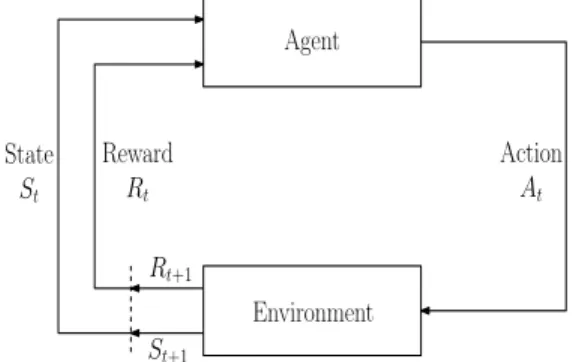
MDP is defined as a stochastic control process, each time, the environment is at a state
St∈ S, and the agent (decision maker) responses by an actionAt∈ A. At the next time slot,
the environment responses by moving into a new random state St+1, and gives the agent a
corresponding reward Rt+1 ∈ R. Figure 2.1 shows the interaction between the agent and the
environment [59]. Agent Environment Action At Rt+1 St+1 Reward Rt State St
In finite MDPs, the sets of states S, actions A, and rewards R have finite numbers of
elements. Rt and St are random variables (RVs) with discrete probability distributions that
depend on the previous state and action only. The mathematical model of finite MDPs can be defined using the following elements [59]:
1. A set of statesS.
2. A set of actionsA.
3. The state-transition probabilities, where p(s0|s, a) is the probability of reaching state
s0∈ S given that action a∈ Ais taken at states∈ S.
4. The expected reward for state-action-next-stater(s, a, s0).
5. The discount factor γ ∈ [0,1] that determines the weight of the immediate reward
compared to future rewards.
Figure 2.2 shows a finite MDP with two states, S = {Tired,Active}. At each state, the
decision maker can decide whether to sleep or work. The action set is A = {Sleep,Work}.
Working in the tired state leaves the agent at the tired state with probability 1 and results in a reward of 0.7. Sleeping in the tired state moves the agent to the active state with probability 1 and 0 reward. On the other hand, if the agent decides to sleep in the active state, it will stay active with probability 1 and get a 0 reward. Deciding to work in the active state results in a reward of 5, leaves the agent in the active state with probability 0.8, and moves it to the tired state with probability 0.2.
Tired Active −−Sleep · · ·Work p= 1,r= 0 p= 1,r= 0:7 p= 0:2,r= 5 p= 0:8,r= 5 p= 1,r= 0
2.2 Problem Formulation of Decision Making in Uncertain Environments
According to [76], a general problem formulation of decision under stochastic uncertainty is described by the system’s state evolution function, a random disturbance depending on the
context, a policy π used to control actions’ selection, and an objective function.
Given an action aselected at states, the state evolution formula is given by
s0 =f(s, a, u) (2.1)
where s0 is the next state, u ∈ U is a random disturbance, U is the disturbance set, and f is
the function that describes the mechanism of evolving the states.
The random disturbance u is characterized by a probability distribution Pr(u|s, a) that
may depend on the current state-action pair. The policy π controls selecting actions at the
available states. A deterministic policy π maps states into a particular action at each state,
π(·) :s→a,∀s. A parameterized stochastic policyπ(a|s,θ) selects each actionawith a certain
probability given a statesand a policy’s parameter vectorθ [59]. π(a|s,θ) is given by
π(a|s,θ) = Pr(a|s,θ) (2.2)
where Pr(·) is a probability distribution describing the probabilities of selecting actions.
Due to the presence of the disturbance u, the objective function J is formulated as the
expected cumulative cost over a period of time. An optimal policy π∗ is the policy that
minimizesJ; that is,
J∗ = min
π∈ΠJ (2.3)
where Π is the set of all admissible policies.
2.3 Value Functions
To evaluate different policies, value functions (state-value function vπ(s) and action-value
function qπ(s, a)) can be used. The state-value function is the expected cumulative reward
starting from state sand then following policyπ thereafter.
vπ(s) =Eπ " ∞ X i=0 γiRt+i+1 St=s # (2.4)
The action-value function of a state-action pair (s, a) is defined as the expected cumulative
reward starting from stateswith actiona, and then following policy π successively [4].
qπ(s, a) =Eπ " ∞ X i=0 γiRt+i+1 St=s, At=a # (2.5)
The optimal policy π∗ has expected cumulative reward that is better than or equal to any
other policyπ in all states (i.e., vπ∗(s)≥vπ(s), ∀s∈ S) [38], where
vπ∗(s) = max
π vπ(s), ∀s∈ S (2.6)
The optimal action-value function is given by
qπ∗(s, a) = max π qπ(s, a), ∀s∈ S,∀a∈ A (2.7) From (2.6), (2.7) vπ∗(s) = max a qπ ∗(s, a), ∀s∈ S (2.8) 2.4 Reinforcement Learning
Machine Learning types are mainly divided into three categories based on their purposes. These categories are supervised learning, unsupervised learning, and RL [77]. In supervised learning, the algorithms are provided by a set of features with their correct labels. Once the mapping of provided features to their labels is learned, it is used to map unseen features to their labels. On the other hand, unsupervised learning aims to extract meaningful representations for data without using labels. In RL, there is an agent interacts with an environment. This interaction results a feedback signal, which is used to modify the agent’s interaction and improve its performance [78; 79].
The main point that characterises RL from other types of learning is that it uses training information for evaluating the taken action. On the other hand, the other types use these
information for instructing by giving correct actions [4]. RL mainly aims at enabling an
autonomous agent to optimize its policy to maximize its total expected reward. Here, the agent is placed in an unknown environment, and learns by trial and error [48].
Exploration and exploitation are fundamental concepts in RL, which are used to optimizes the agent’s policy. At any time, there is at least one action for each state with the highest
estimated value, this action is called a greedy action. If the greedy action is selected, this mode is called exploitation, where the agent exploits its current knowledge to determine the current best action (i.e. greedy action). On the other hand, when a nongreedy action is selected, this mode is called exploration. Using exploration, the agent can improve its estimates about nongreedy actions, and discover actions with higher values than the greedy action [4]. Balancing between exploration and exploitation is an important factor affecting the cumulative rewards. Balancing is one of the main challenges facing RL, and it is known as the exploration-exploitation dilemma [4; 49].
Methods used for learning an optimal policy in RL can be categorized into two main classes, which are value-based RL methods, and policy gradient RL methods. Value-based RL is defined as methods that learn the values of actions, and then, select actions according to the estimated actions’ values (i.e., policies are extracted from the estimated actions’ values). Value-based methods use a sequence of policy evaluation and policy improvement cycles. Policy evaluation is used to estimate a value function for the agent’s current policy, while policy improvement is used to improve the policy based on the new estimated value function [59]. Temporal difference (TD) learning is one of the well known value-based reinforcement learning methods. The idea of the TD methods is to estimate a value function from the difference between temporally successive estimates. State-action-reward-state-action (SARSA) is an example of TD prediction methods, which estimates values of state-action pairs according to
Q(s, a)←Q(s, a) +α(r(s, a, s0) +γ Q(s0, a0)−Q(s, a)) (2.9)
where α is the learning rate, Q(s, a) is the estimate of the current state-action pair (s, a),
Q(s0, a0) is the estimate of the next state-action pair (s0, a0), r(s, a, s0) is the reward resulting
from taking actionaat states, andδ = (r(s, a, s0) +γ Q(s0, a0)−Q(s, a)) is the TD error, which
is the difference between the target (r(s, a, s0) +γ Q(s0, a0)) and the current predictionQ(s, a).
Policy gradient RL is defined as methods learning a parameterized policy, which is able to select actions without consulting a value function. Using this type of learning, value functions may be used to learn the policy’s parameters, but they are not needed for actions selection [59]. Policy gradient methods are characterized by a number advantages, which are summarized as
follows. The first one is the ability to learn mixed strategies, which are balanced stochastically. The second one is their convergence properties, which are better than those of value-based methods. They are able to converge to at least a local optimal policy. The third advantage is their capability of learning in problems with continuous action spaces [80]. One of the well known policy gradient learning algorithms is the REINFORCE [81]. This algorithm uses a
differentiable policy π(a|s,θ) parameterised by a vector of adjustable weights θ. Stochastic
gradient ascent is used to optimize θ to maximize a policy performance measure.
Actor-critic (AC) are learning algorithms combining value-based and policy gradient RL methods. AC algorithms mainly consist of an actor and a critic. The actor estimates a value function, while the critic optimizes the policy’s parameters.
CHAPTER 3. COGNITIVE RADIO NETWORKING WITH ENERGY HARVESTING AND COOPERATIVE RELAYING
In this chapter, an underlay cognitive radio energy harvesting (CR-EH) system assisted by a decode and forward (DF) relay is considered, where the secondary users can access the primary user frequency band by exploiting the allowance of its signal-to-interference-plus-noise ratio (SINR) constraints. Moreover, both the secondary source and relay are considered as buffer-aided nodes that can buffer infinite data and store finite energy. The main goal of this work is to derive the optimal power policy that maximizes the number of bits received by the secondary destination. Finally, the performance of the proposed scheme is analyzed to verify our findings, and compared with other schemes to check its validity and efficiency.
The remainder of this chapter is organized as follows. Section 3.1 describes the proposed
EH-CR system. The problem formulation is given in Section3.2. Then, the proposed solution
is discussed in Section 3.3. Numerical simulation results are presented in Section3.4. Finally,
this chapter is concluded in Section 3.5.
3.1 System Model
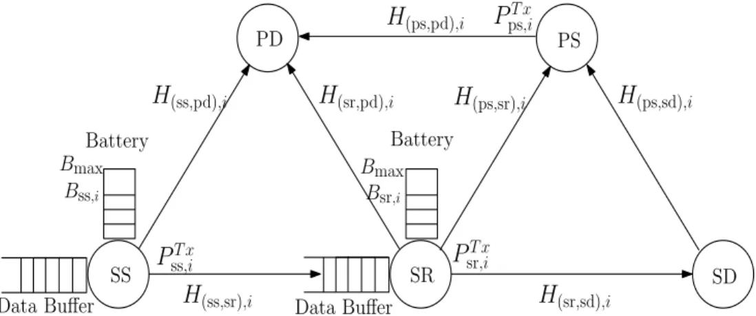
We consider a cooperative CRN with EH consisting of primary and secondary networks,
as illustrated in Figure 3.1. The primary network consists of primary source and destination
nodes, denoted by PS and PD, respectively. The secondary network is a two-hop relay network consisting of a source, a relay, and a destination node denoted by SS, SR and SD, respectively. SS and SD are far away from each other, i.e., they are not in the coverage communication range of each other. Each of the SS and SR is equipped with infinite data queue to buffer received data and finite battery to store harvested energy. It is assumed that there are always data
packets in the data queue of the SS to be delivered to the SD, which causes depletion of the energy of the SS. Data packets are sent from SS to SR and then are transmitted from the SR to the SD, which causes depletion of the SR’s energy. The SR is a full-duplex node, which can transmit and receive data at the same time. In this model, energy consumption is considered only due to data transmission, and it does not take into account any other energy consumption, such as processing, circuitry, etc.
Battery Bmax Bsr;i Battery Bmax Bss;i Data Buffer Data Buffer SR SD PS PD SS
H
(sr,pd);iH
(ps,pd);iH
(ps,sd);iH
(ss,pd);iH
(ps,sr);iH
(sr,sd);iH
(ss,sr);iP
srT x;iP
psT x;iP
ssT x;iFigure 3.1: Cooperative underlay CR system with EH.
We consider a time slotted system withT equal length time slots. In the secondary network,
a DF relaying protocol is used, where the SR can decode the SS signal before broadcasting it to the SD. It is assumed that updating the data queue and energy storage of the SR is delayed by one time slot with respect to the SS. Because of this delay, the efficiency of data transfer
from the SS to SD is affected slightly. We assume that T is large so that the slight loss of
inefficiency can be neglected.
Let the maximum capacity of the batteries be Bmax. Bss,i and Bsr,i represent the battery
levels of both SS and SR, respectively, at time sloti. Each time slot is divided into two equal
sub-slots for both transmitting and harvesting. Figure3.2illustrates the slotted system model
for both SS and SR. This model is designed such that the EH nodes first transmit their signals and then harvest energy, where the transmit power in the current slot depends only on the previous battery level. The batteries are assumed to be ideal, which means that there is no loss during retrieving or storing energy.
Bi−1 Bi
Tc Tc
PiT x Ei
Transmission duration Harvesting duration
Figure 3.2: Slotted system model for EH nodes.
The channels are Rayleigh fading channels. It is also assumed that we have full channel
state information (CSI), and the channels are stationary within every time slot, i.e.,H(x,y),i is
constant during theith time slot, where the channel between the nodes x and y at time sloti
is given by
H(x,y),i=
q
dαpl
(x,y)H˜(x,y),i (3.1)
whered(x,y)is the distance between the two nodes,αplis a path loss constant, and ˜H(x,y),iis the
fading coefficient between x and y. Let us similarly defineH(ss,sr),i,H(sr,sd),i,H(ss,pd),i,H(sr,pd),i,
H(ps,pd),i, H(ps,sd),i and H(ps,sr),i as the channel coefficients during the ith time slot between SS and SR, SR and SD, SS and PD, SR and PD, PS and PD, PS and SD, and PS and SR,
respectively. The harvested energy at SS and SR during the ith time slot are denoted by Ess,i
and Esr,i, respectively. Two transmission cases are studied, case 1) SS keeps transmitting its
data for all of the T slots, case 2) SS completes its transmission withinM slots whereM < T,
after that, it keeps harvesting forT −M slots without sending data to the SR. This gives the
SR extra time T −M to try sending all the data in its buffer. The latter case allows SR to
receive data from the SS but not transmit them to the SD due to channel conditions, primary interference, or lack of harvested energy at the SR.
3.2 Problem Formulation
It is assumed that the PS transmits to the PD during all time slots. So, the received signal
and the SINR at the PD side during the ith slot are, respectively, given as
ypd,i= q PT x ps,i H(ps,pd),i xps,i+ q PT x ss,i H(ss,pd),i xss,i + q PT x sr,i H(sr,pd),i xsr,i+npd,i, i= 1, . . . , T (3.2)
Γpd,i= PT x ps,i|H(ps,pd),i|2 σ2 n+PssT x,i|H(ss,pd),i|2+PsrT x,i|H(sr,pd),i|2 , i= 1, . . . , T (3.3)
where PpsT x,i and xps,i are the peak transmit power, and the transmitted signal by PS,
respectively. npd,i is additive Gaussian noise with zero-mean and noise variance σn2. The
received signals at the SR and the SD duringith slot are, respectively, given as
ysr,i= q PT x ss,iH(ss,sr),ixss,i+ q PT x ps,iH(ps,sr),ixps,i+nsr,i, i= 1, . . . , M (3.4) ysd,i= q PT x sr,iH(sr,sd),ixsr,i+ q PT x ps,iH(ps,sd),ixps,i+nsd,i, i= 1, . . . , T (3.5)
wherePssT x,i andPsrT x,i are the peak power transmitted by SS and SR, respectively. xss,iand xsr,i
are the transmitted signals by SS and SR during the ith time slot, respectively. We assume
thatnsr,i andnsd,iare Gaussian, independent, zero mean, and they both also have varianceσ2n.
The SINR at the SR and SD are given, respectively, by
Γsr,i= PssT x,i|H(ss,sr),i|2 σ2 n+PpsT x,i|H(ps,sr),i|2 , i= 1, . . . , M (3.6) Γsd,i= PsrT x,i|H(sr,sd),i|2 σ2 n+PpsT x,i|H(ps,sd),i|2 , i= 1, . . . , T (3.7)
where the SR can remove the self interference by eliminating its own signal.
The objective is to optimize transmit powers for both SS and SR in order to maximize the
sum rate between the SR and SD duringT time slots, while satisfying the required QoS of the
primary users, in addition to the data and energy causality constraints. The sum rate from SR to SD is given by max {PT x ss,i,PsrT x,i,Bss,i,Bsr,i} T X i=1 log(1 + Γsd,i) (3.8)
Thus, the energy causality constraints at SS and SR (i.e., the SS and SR cannot use more energy than their battery levels in the previous time slot), respectively, are given by
PssT x,iTc≤Bss,i−1, i= 1, . . . , T (3.9)
PsrT x,iTc≤Bsr,i−1, i= 1, . . . , T (3.10)
where Tc is the transmission duration. Since SS will keep silent (i.e. PssT x,i = 0) after time slot
Battery overflow constraints for both SS and SR (i.e., the update rules for the available energy in their batteries at the end of the current time slot, which are functions of the previous battery levels, in addition to transmit and harvested energy in the current time slot), respectively, are given by
Bss,i= min{Bss,i−1+Ess,i−PssT x,iTc, Bmax}, i= 1, . . . , T (3.11)
Bsr,i= min{Bsr,i−1+Esr,i−PsrT x,iTc, Bmax}, i= 1, . . . , T (3.12)
Constraints (3.11) and (3.12) can be rewritten as follow
Bss,i≤Bss,i−1+Ess,i−PssT x,iTc, i= 1, . . . , T (3.13)
Bss,i≤Bmax, i= 1, . . . , T (3.14)
Bsr,i≤Bsr,i−1+Esr,i−PsrT x,iTc, i= 1, . . . , T (3.15)
Bsr,i≤Bmax, i= 1, . . . , T (3.16)
PssT x,i,PsrT x,i,Bss,i andBsr,i should satisfy the following constraints
PssT x,i ≥0, i= 1, . . . , M (3.17)
PssT x,i = 0, i=M+ 1, . . . , T (3.18)
PsrT x,i ≥0, i= 1, . . . , T (3.19)
Bss,i, Bsr,i ≥0, i= 1, . . . , T (3.20)
Without loss of generality, and for simplicity, it is assumed that Tc is normalized, hence, it
is omitted from the following equations. The following constraint is to ensure the data causality (i.e., the SR will not transmit the data to the SD before receiving it)
i X k=1 log(1 + Γsd,k)≤ i X k=1 log(1 + Γsr,k), i= 1, . . . , M (3.21)
The data queue of the SR increases by log(1 + Γsr,k) bit/Hz in the following time slot, when
the SS transmits with PssT x,i to the SR during the ith slot. The same observation can be made
at SD when the SR transmits with PsrT x,i.
To grantee a QoS to the primary network, the following constraint should be satisfied Γpd,i≥Γ, i= 1, . . . , T (3.22)
where Γ is the predefined SINR QoS threshold at the PD. With simple manipulations, constraint
(3.22) can be rewritten as
PssT x,i|H(ss,pd),i|2+PT x
sr,i|H(sr,pd),i|2 ≤Ith,i, i= 1, . . . , T (3.23)
whereIth,iis given by
Ith,i=
PpsT x,i|H(ps,pd),i|2
Γ −σ
2
n, i= 1, . . . , T (3.24)
Finally, the following constraint requires that the received data at SD during T −M slots
(during the time where the SS is not transmitting) is limited by the data in the SR buffer
T X i=1 log(1 + Γsd,i)≤ M X i=1 log(1 + Γsr,i) (3.25)
The end-to-end rate optimization problem that maximizes the sum rate between SR and SD can now be formulated as
max {PT x ss,i,PsrT x,i,Bss,i,Bsr,i} T X i=1 log(1 + Γsd,i) subject to (3.9)–(3.10),(3.13)–(3.21),(3.23),(3.17)–(3.25) (3.26) 3.3 Proposed Solution
The formulated optimization problem given in (3.26) is a non convex problem because of
constraints (3.21) and (3.26). In the sequel, we will transform it to an equivalent convex form.
Change of variables can be used as follows [22]. LetCsr,i = log(1 + Γsr,i),Csd,i= log(1 + Γsd,i).
For simplicity, let us define the following
ςi = σn2+PpsT x,i|H(ps,sr),i|2 |H(ss,sr),i|2 , i= 1, . . . , M (3.27) ϑi= σ2 n+PpsT x,i|H(ps,sd),i|2 |H(sr,sd),i|2 , i= 1, . . . , T (3.28)
From (3.6), (3.7), (3.27), and (3.28), PssT x,i and PsrT x,i can be written, respectively, as follows
PssT x,i =ςiΓsr,i (3.29)
Therefore, the formulated optimization problem after transformation can be written as max {Csd,i,Csr,i,Bss,i,Bsr,i} T X i=1 Csd,i i X k=1 Csd,k ≤ i X k=1 Csr,k, i= 1, . . . , M ςi(2Csr,i−1)≤Bss,i−1, i= 1, . . . , T ϑi(2Csd,i −1)≤Bsr,i−1, i= 1, . . . , T Bss,i≤Bss,i−1+Ess,i−ςi(2Csr,i−1), i= 1, . . . , T Bss,i≤Bmax, i= 1, . . . , T Bsr,i≤Bsr,i−1+Esr,i−ϑi(2Csd,i−1), i= 1, . . . , T Bsr,i≤Bmax, i= 1, . . . , T T X i=1 Csd,i≤ M X i=1 Csr,i ςi(2Csr,i−1)|H(ss,pd),i|2+ϑi(2Csd,i −1)|H(sr,pd),i|2≤Ith,i, i= 1, . . . , T 2Csr,i −1≥0, i= 1, . . . , M 2Csr,i −1 = 0, i=M + 1, . . . , T 2Csd,i −1≥0, i= 1, . . . , T Bss,i, Bsr,i≥0, i= 1, . . . , T (3.31)
Now to transform the problem to a convex one, the last three constraints can be rewritten, respectively, as
−Csr,i≤0, i= 1, . . . , M (3.32)
Csr,i= 0, i=M+ 1, . . . , T (3.33)
−Csd,i≤0, i= 1, . . . , T (3.34)
Hence, the optimization problem becomes a convex problem, where the objective function
is concave and the constraints are convex functions [82]. The Lagrangian of (3.31) is given in
L=− T X i=1 Csd,i+ M X i=1 µi hXi k=1 (Csd,k−Csr,k) i + T X i=1 θi h ςi(2Csr,i−1)−Bss,i−1 i + T X i=1 ωi h ϑi(2Csd,i −1)−Bsr,i−1 i + T X i=1 ηi h Bss,i−Bss,i−1−Ess,i+ςi(2Csr,i −1) i + T X i=1 λi h Bsr,i−Bsr,i−1−Esr,i+ϑi(2Csd,i −1) i + T X i=1 κi h Bss,i−Bmax i + T X i=1 φi h Bsr,i−Bmax i − M X i=1 σiCsr,i+ T X i=M+1 νiCsr,i+ξ hXT k=1 Csd,k− T X k=1 Csr,k i + T X i=1 ψi h ςi(2Cr,i−1)|H(ss,pd),i|2+ϑi(2Csd,i −1)|H(sr,pd),i|2−Ith,i i − T X i=1 ρiCsd,i− T X i=1 ϕiBss,i− T X i=1 %iBsr,i (3.35)
The Karush-Kuhn-Tucker (KKT) conditions are given as follows
− M X i=k µi−σk−ξ+ςkln(2)2Csr,k n θk+ηk+ψk|H(ss,pd),k|2 o = 0, k= 1, . . . , M (3.36) νk+ςkln(2)2Csr,k n θk+ηk+ψk|H(ss,pd),k|2 o = 0, k=M + 1, . . . , T (3.37) −1 + M X i=k µi−ρk+ξ+ϑk(ln(2))2Csd,k n ωk+λk+ψk|H(sr,pd),k|2 o = 0, k= 1, . . . , M (3.38) −1−ρk+ξ+ϑk(ln(2))2Csd,k n ωk+λk+ψk|H(sr,pd),k|2 o = 0, k=M + 1, . . . , T (3.39)
Using (3.36) - (3.39), the closed form expressions can be obtained as
Csr∗,k = (csr,1)+, k= 1, . . . , M (csr,2)+, k=M+ 1, . . . , T (3.40) Csd∗,k = (csd,1)+, k= 1, . . . , M (csd,2)+, k=M+ 1, . . . , T (3.41)