Rowan University Rowan University
Rowan Digital Works
Rowan Digital Works
Theses and Dissertations 8-17-2017Learning extreme verification latency quickly with importance
Learning extreme verification latency quickly with importance
weighting: FAST COMPOSE & LEVEL_IW
weighting: FAST COMPOSE & LEVEL_IW
Muhammad Umer Rowan University
Follow this and additional works at: https://rdw.rowan.edu/etd Part of the Electrical and Computer Engineering Commons
Let us know how access to this document benefits you -
share your thoughts on our feedback form.
Recommended Citation Recommended Citation
Umer, Muhammad, "Learning extreme verification latency quickly with importance weighting: FAST COMPOSE & LEVEL_IW" (2017). Theses and Dissertations. 2465.
https://rdw.rowan.edu/etd/2465
This Thesis is brought to you for free and open access by Rowan Digital Works. It has been accepted for inclusion in Theses and Dissertations by an authorized administrator of Rowan Digital Works. For more information, please contact [email protected].
LEARNING EXTREME VERIFICATION LATENCY QUICKLY WITH IMPORTANCE WEIGHTING: FAST COMPOSE & LEVELIW
by
Muhammad Umer
A Thesis Submitted to the
Department of Electrical & Computer Engineering College of Engineering
In partial fulfillment of the requirement For the degree of
Master of Science in Electrical & Computer Engineering at
Rowan University August 09,2017
Dedication
Acknowledgements
I would like to thank my advisor and mentor, Professor Robi Polikar, whose en-thusiasm and vision in research has greatly inspired me, and whose constant guidance and encouragement has made this work possible. I also would like to extend my gratitude to Dr. Ravi Prakash Ramachandran and Dr. Umashangar Thayasivam for being part of my committee and for their generous time and commitment. Special thanks to Christopher Frederickson, who has been very helpful in paper reviews and code development. Finally, I would like to thank my family who has always supported and encouraged me to continue moving forward throughout my academic career.
Abstract Muhammad Umer
LEARNING EXTREME VERIFICATION LATENCY QUICKLY WITH IMPORTANCE WEIGHTING: FAST COMPOSE & LEVELIW
2016-2017 Robi Polikar, Ph.D.
Master of Science in Electrical & Computer Engineering
One of the more challenging real-world problems in computational intelligence is to learn from non-stationary streaming data, also known as concept drift. Perhaps even a more challenging version of this scenario is when – following a small set of initial labeled data – the data stream consists of unlabeled data only. Such a scenario is typically referred to as learning in initially labeled nonstationary environment, or simply as extreme veri-fication latency (EVL). This thesis introduces two different algorithms to operate in this domain. One of these algorithms is a simple modification of our prior work, COMPOSE (COMPacted Object Sample Extraction), that allows the algorithm to work without its ex-tremely computationally expensive core support extraction module. We call this modified algorithm FAST COMPOSE. The other algorithm we propose that works in this setting is based on the importance weighting domain adaptation approach. We explore impor-tance weighting to match distributions between two consecutive time steps, and estimate the posterior distribution of the unlabeled data using importance weighted least squares probabilistic classifier. The estimated labels are then iteratively used as the training data for the next time step. We call this algorithm LEVELIW, short for Learning Extreme
VEr-ification Latency with Importance Weighting. An additional important contribution of this thesis is a comprehensive survey and comparative analysis of competing algorithms to point out the weaknesses and strengths of different approaches from three different perspectives: classification accuracy, computational complexity and parameter sensitivity using several synthetic and real world datasets.
Table of Contents
Abstract . . . v
List of Figures . . . viii
List of Tables . . . ix
Chapter 1: Introduction . . . 1
1.1 Motivation: Learning in Non-Stationary Environments . . . 1
1.2 Problem Statement . . . 2
1.3 Scope of Thesis . . . 3
1.4 Research Contributions . . . 4
1.5 Organization of the Thesis . . . 5
Chapter 2: Background . . . 7
2.1 Concept Drift . . . 7
2.1.1 Single Classifier vs. Ensemble Classifier Based Approaches for Concept Drift . . . 8
2.1.2 Active vs. Passive Approaches for Concept Drift . . . 9
2.2 Domain Adaptation . . . 10
2.2.1 Unsupervised Domain Adaptation and Importance Weighting . . . . 12
2.2.2 Supervised Domain Adaptation . . . 20
2.3 Transfer Learning . . . 22
2.3.1 Inductive Transfer Learning . . . 22
2.3.2 Transductive Transfer Learning . . . 23
2.4 Verification Latency . . . 23
Chapter 3: Preliminary and Related Work . . . 27
Table of Contents(Continued)
3.2 Stream Classification Algorithm Guided by Clustering (SCARGC) . . . 32
3.3 Micro-Cluster for Classification (MClassification) . . . 36
3.4 COMPOSE.V1 (Original COMPOSE Withα-Shape Construction) . . . 39
3.5 COMPOSE.V2 (COMPOSE With Gaussian Mixture Model (GMM) or Any Density Estimation Technique) . . . 42
Chapter 4: Improving Learning Concept Drift Under Extreme Verification Latency: Learning Extreme Verification Quickly With FAST COMPOSE and With Importance Weighting (LEVELIW) . . . 46
4.1 The Underlying Problems With Current Approaches . . . 46
4.2 Learning Extreme Verification Latency Quickly: FAST COMPOSE . . . 51
4.3 LEVELIW: Learning Extreme VErification Latency With Importance Weighting . . . 53
4.3.1 Importance Weighted Least-Squares Probabilistic Classifier . . . 55
4.3.2 LEVELIW . . . 61
Chapter 5: Experiments, Results and Comprehensive Analysis of Algorithms for Learning Under Extreme Verification Latency . . . 64
5.1 Analysis of Three Versions of COMPOSE . . . 71
5.2 Analysis of SCARGC . . . 75
5.3 Analysis of MClassification . . . 77
5.4 Analysis of LEVELIW . . . 82
5.5 Analysis on two Additional Real World Datasets . . . 85
Chapter 6: Conclusion and Future Work . . . 95
6.1 Summary of Future Work . . . 98
List of Figures
Figure Page
Figure 1. Graphical representation of covariate shift and class imbalance . . . 18
Figure 2. Graphical representation of verification latency . . . 24
Figure 3. Graphical representation of extreme verification latency scenario . . . 25
Figure 4. Block diagram and Graphical Representations of APT . . . 31
Figure 5. Block diagram and Graphical Representations of SCARGC . . . 34
Figure 6. Block diagram and Graphical Representations of MClassification . . . 39
Figure 7. Block diagram and operation workflow of COMPOSE . . . 43
Figure 8. Example depicting core support extraction procedure in COMPOSE . . . 50
Figure 9. Block diagram and graphical illustration of FAST COMPOSE . . . 53
Figure 10. Block diagram and graphical representation of LEVELIW . . . 62
Figure 11. Progress of drift for 1CDT, 1CHT, 2CDT, and 2CHT datasets . . . 67
Figure 12. Three different snapshots of GEARS 2C 2D data . . . 68
Figure 13. Three different snapshots of UG 2C 3D data . . . 68
Figure 14. Progress of drift for 4CR, 4CRE-V2, 1Csurr, and 4CE1CF datasets . . . . 69
Figure 15. Four different snapshots of5CVTdataset . . . 72
Figure 16. Accuracy Comparison of COMPOSE on balanced 5CVT dataset . . . 73
Figure 17. Classification accuracy comparison of SCARGC on 5CVT dataset . . . . 76
Figure 18. Six Snapshots ofF G 2C 2Ddata . . . 78
Figure 19. Accuracy of Algorithms onF G 2C 2Ddata . . . 79
Figure 20. Six Snapshots ofM G 2C 2Ddata . . . 80
Figure 21. Accuracy of Algorithms onM G 2C 2Ddata . . . 81
Figure 22. UG 2C 2D data for six different snapshots . . . 83
Figure 23. Accuracy of algorithms onU G 2C 2Ddata . . . 84
Figure 24. Accuracy of algorithms on real worldweatherdata . . . 87
Figure 25. Sample images of traffic scenes streaming from a traffic camera . . . 87
List of Tables
Table Page
Table 1. Dataset descriptions . . . 66
Table 2. Average classification accuracy . . . 90
Table 3. Average execution time (in seconds) . . . 91
Table 4. Statistical significance atα = 0.05for classification accuracy . . . 91
Table 5. Statistical significance atα = 0.05for execution time . . . 92
Table 6. Accuracy with three different values of k (SCARGC) . . . 92
Table 7. Accuracy with three different values ofrfor (MClassification) . . . 93
Table 8. Accuracy with three different values of k (COMPOSE) . . . 93
Chapter 1 Introduction
1.1 Motivation: Learning in Non-Stationary Environments
The fundamental goal in machine learning is to learn from data. Depending on the availability of labeled data, machine learning can be broadly categorized into three categories, namely supervised learning (where sufficient amount of labeled data are avail-able for training), unsupervised learning (where only unlabeled data are availavail-able), and semi-supervised learning (where some labeled data and some unlabeled data are available). Most machine learning algorithm, regardless of the availability of labeled data, make a fundamental assumption that data are drawn from a fixed but unknown distribution. This assumption implies that test or field data come from the same distribution as the training data. In reality, this assumption simply does not hold in many real world problems that generate data whose underlying distributions change over time. Network intrusion, web usage and user interest analysis, natural language processing, speech and speaker identifi-cation, spam detection, anomaly detection, analysis of financial, climate, medical, energy demand, or pricing data, as well as the analysis of signals from autonomous robots and devices, brain signal analysis, and bio-informatics are just a few examples of the real world problems where underlying distributions may – and typically do – change over time.
In machine learning, the challenge of making decisions in a changing environment is referred to as non-stationary learning. This is a challenging problem, because the classi-fier needs to adapt to a new concept in the changing environment, while retaining the pre-viously acquired knowledge that is still relevant to ensure a stable learning environment, a phenomenon commonly referred to as the stability-plasticity dilemma in literature [1].
The fixed distribution assumption, essentially requiring the data to be drawn independently from an identical distribution (also referred to as independent and identically distributed -i.i.d.) renders traditional learning algorithms that make this assumption ineffective at best, misleading and inaccurate at worst on non-stationary distribution problems.
1.2 Problem Statement
Concept drift techniques [2–7] and domain adaptation approaches [8, 9] have been developed to tackle two related but different issues related to non-stationary distributions: domain adaptation techniques are designed to handle mismatched training and test distri-bution over a single time-step, while concept drift approaches are designed to track the data distributions over a streaming setting. However, both approaches assume that there is (preferably ample) labeled training data, and the potential scarcity or the high cost of obtaining labeled data is a major obstacle faced by these approaches.
In an effort to reduce the amount of required labeled data, semi supervised learning (SSL) approaches have also been employed, where a hypothesis is formed using modest amount of labeled data and more abundant unlabeled data. SSL approaches, of course, also require labeled data at each time step [10], albeit in smaller quantities. Active learning (AL) is another approach to combat the limited availability of labeled data [11], where the learner actively chooses which data instances – if labeled – would provide the most benefit. The goal in AL algorithms is therefore to find the minimum number of labeled examples that provide the maximum benefit. This is most commonly achieved by assuming that there is an oracle or expert that can be queried for the labels of any example on demand. Active learning approaches cannot function, however, if the requested labels cannot be provided
on demand, a potentially restricting limitation.
The unavailability of labeled data, particularly in streaming applications, gives rise to another problem, commonly referred to as verification latency in the literature [12], where labeled data are not available at every time step. More specifically, verification latency refers to the scenario where labels of the training data becoming available only certain or some unspecified amount of time later, significantly complicating the learning process. The duration of the lag in obtaining labeled data may not be known a priori, and/or may vary with time. The extreme case of this phenomenon, aptly named as the
extreme verification latency, is perhaps the most challenging case of all machine learning problems: labels for the training data are never available - except perhaps those provided initially, yet the classification algorithm is asked to learn and track a drifting distribution with no access to labeled data. This thesis explores solutions to this problem of learning from non-stationary and streaming environments in the presence of extreme verification latency.
1.3 Scope of Thesis
The primary goal of this thesis is to develop effective (in terms of classification performance) and efficient (in terms of computational cost associated with the algorithm) approaches for learning in extreme verification latency (EVL). EVL refers to the scenario where obtaining labeled data is expensive or impractical and – perhaps beyond an initial investment – only unlabeled data are available in all future time-steps of a non-stationary data stream. We refered to this scenario as initially labeled non-stationary environment
Arbitrary Sub-Population Tracker (APT); [14], ii) COMPacted Object Sample Extraction (COMPOSE) [13]; iii) Stream Classification Algorithm Guided by Clustering (SCARGC) [15]; iv) and Micro-cluster for Classification (MClassification) [16].
The specific focus of this thesis is not only to develop cost effective and time ef-ficient approaches in this setting, but also to compare and contrast existing approaches, determine if they can be improved through appropriate modifications. Within this setting, we also investigate whether domain adaptation approaches – typically designed to work for single time-step distribution mismatch problems – can be modified to work in streaming setting, and more importantly under EVL.
1.4 Research Contributions
The primary focus of this thesis, as mentioned above, is to develop effective and efficient approaches for learning under extreme verification latency in non-stationary envi-ronments, and compare the performances of the small set of algorithms that are designed to work in similar settings. The core contributions and findings of this work are as follows:
1. FAST COMPOSE is introduced as a very efficient algorithm that can work under extreme verification latency. FAST COMPOSE is a modification of the algorithm COMPOSE, previously developed by Dyer and Polikar [13], where its computation-ally expensive core support extraction module is replaced by using all of the instances labeled by the algorithm in the previous time-step.
2. We observe thatimportance weightingbased domain adaptation approaches can be used for streaming data concept drift problems associated with extreme verification latency when the class conditional distributions at the consecutive time steps share
support.
3. A modification of the well-known importance weighted least squares probabilistic classifier is introduced so that it can work within a) streaming data environment and b) when there is extreme verification latency. The proposed approach is called Learning Extreme VErification Latency with Importance Weighting (LEVELIW).
4. One of the most important contributions of this thesis is to provide a detailed and comprehensive comparison and analysis of competing algorithms used in extreme verification latency setting from three different perspectives: accuracy, computa-tional complexity, and parameter sensitivity. We find that FAST COMPOSE is the best algorithm among others with respect to accuracy and computational complexity, while LEVELIWis the best algorithm with respect to the parameter sensitivity.
1.5 Organization of the Thesis
Chapter 2 provides an overview and background for learning in nonstationary en-vironments, concept drift, domain adaptation and ensemble approaches used for concept drift. Existing approaches for learning in non-stationary environments under extreme veri-fication latency setting are discussed in detail in Chapter 3. Chapter 4 introduces the new algorithms developed as part of this thesis, specifically, FAST COMPOSE developed to learn in extreme verification latency setting quickly; and LEVELIW that extends covariate
shift based domain adaptation approaches to learning under EVL. Chapter 5 presents the experimental setup and results, comparing and analyzing competing algorithms for non-stationary learning under extreme verification latency from three different perspectives: accuracy, computational complexity, and parameter sensitivity. Finally, the conclusions
Chapter 2 Background
This chapter provides a comprehensive background review and technical details of two primary areas that related to learning in non-stationary environments, namely concept drift and domain adaptation. The general overview of these topics along with the connec-tion and concerns with verificaconnec-tion latency are also discussed in this chapter.
2.1 Concept Drift
Concept drift refers to the scenario where the statistical properties of the data change over time in unforeseen ways. Concept drift is not a trivial problem because it occurs within the streaming data which is usually unlabeled and unstructured. The drift scenarios can be abrupt or gradual, slow or fast, random or systematic, cyclical or otherwise. Changes can also be perceived, rather than real, due to insufficient, unknown or unobservable features -referred to as hidden context, where an underlying unknown phenomenon provides a true and static description over time [17],[18]. Concept drift problems typically assume at least a gradual (or limited) drift assumption, but do not require stationary posteriors or same support. So in concept drift we normally havept+1(y|x)6=pt(y|x)wherept+1(x) =pt(x)
may or may not be satisfied. IN other words, the posterior distribution of the data at time
t + 1 may be different from that at time t, while marginal distribution may or may not remain the same as well. This scenario is also known asreal drift.
Data is presented in streams to the concept drift handling algorithms in normally two different ways: i. Online setting- where a single instance is provided to the learner at each time-step, and the learner has to adapt to the change using this single instance; and
ii. batch setting- where several instances are accumulated from the stream, which are then presented to the learner. Online setting is normally considered to be a more challenging learning scenario than the batch setting because less data (i.e. single instance at each time-step) makes it difficult for the learner to adapt to the changes easily. On the other hand, batch learners often lag in reacting to changing concepts because it is often assumed that concept does not change within the given batch of data. Of course, the stationarity within a batch assumption is rarely true.
Concept drift algorithms can be characterized in various ways; such as single clas-sifier vs. ensemble-based approaches, or active vs. passive approaches.
2.1.1 Single classifier vs. Ensemble classifier based approaches for Concept drift. Single-classifier approaches learn the drifting concept by either replacing the cur-rent classifier with a new classifier trained on newly received data, or updating the ad-justable parameters of a given classifier to reflect changes present in newly received data [19],[20], [21]. Single classifier approaches are more prone to stability-plasticity dilemma: an entirely stable learner would not be able to learn changing environment and an entirely plastic learner would not be able to deal with catastrophic forgetting [22], i.e. it would not be able to retain any of the previous knowledge that may still be relevant. Learning algorithms based on single-classifier approaches strive to balance stability and plasticity.
On the other hand, ensemble based approaches use a combination of several clas-sifiers to make a decision, hence minimizing the stability-plasticity problems, albeit at in-creased computational cost. Ensemble approaches track the environment by adding new classifiers with each incoming dataset to build a family of classifiers. These approaches
minimize the stability-plasticity dilemma concerns by providing both stability (a subset or all of the prior classifiers can be retained or reweighted) and plasticity (learning new in-formation by adding new classifiers). A fixed or dynamic ensemble size may be used by these approaches. For fixed ensemble size, either the oldest member [23], [24] or the least contributing ensemble member is replaced with a new one as done in Dynamic Weighted Majority (DWM) algorithm in [25]. If dynamic ensemble size is being used, additional classifiers can be added without removing existing classifiers (though they would often be reweighted to reduce their impact). Weighted [26] or simple majority [27] voting are the most common approaches for combining the classifiers when an ensemble approach is used. Abdulsalam et al.’s random forests with entropy [28], Masud et al.s concept drift with time constraints [29], Bifets integration of a Kalman filter with Adaptive Sliding Win-dow (ADWIN) [30], and Massive Online Analysis [31] represent ensemble approaches that combine ensemble of classifiers and sliding window techniques. Learn++.NSE [32], [4], and Learn++.NIE [5] represent a more modern family of approaches for mining data
streams with concept drift that do not rely on sliding window, and can dynamically deter-mine which ensemble members are relevant at any given time.
2.1.2 Active vs. Passive approaches for Concept drift. In active approaches, the algorithm continuously monitors the data to determine if and when change occurs. If – and only if – a change is detected, the algorithm takes an appropriate action, such as updating the classifier with the most recent data or simply creating a new classifier to learn the current data, depending on the nature of the algorithm. Passive approaches, on the other hand, do not explicitly monitor the data for change, but rather assume change may occur
at any time new data become available. A passive algorithm therefore updates the model every time new data arrive, regardless of the presence of change/drift. There are a multitude of active drift detection approaches. Many of the earliest algorithms for concept drift were Window based approaches, such as STAGGER [33], FLORA [17], and their variants. These algorithms use a sliding window to choose a block of new data to train a new classifier when change was detected and are example of active drift detection approaches. Other approaches include statistical control charts as used in Alippi and Roveri’s just-in-time (JIT) classifiers[34], and the more recent intersection of confidence intervals (ICI) rule [35]. Information theoretic measures [36], Hoeffding bounds or Hellinger distance [37], [38] are other active approaches that are based on monitoring classifier’s accuracy or some metric to detect the change and updating the classifier.
2.2 Domain Adaptation
Domain adaptation refers to the learning scenario when the data distribution used to train the model is different than that of the data on which the learner needs to predict. Within the context of domain adaptation, the training data is referred to as source data, whereas the test or field data is known as thetarget data, with the corresponding data dis-tributions being referred to as source and target data disdis-tributions, respectively. Domain adaptation problems are typically not associated with streaming data as there is only a sin-gle time step. Examples of domain adaptation problems include, e.g.,speaker identification
where the source data distribution may vary from that of the target data due to the recording environment change, physical conditions/emotions, and session-dependent variations [39]. Another example is brain-computer interface (BCI), which allows direct communication
from human brain to machine to control an external entity [40]. Electroencephalography (EEG) is often the signal of choice in BCI applications, and EEG signals are known to be extremely nonstationary [41]. In BCI experiments, training samples and unlabeled test samples are usually gathered in different recording sessions, and the non-stationarity in the brain signals can cause a change in the distributions rendering the classifier update neces-sary in this setting. Natural language processing (NLP) is another case, where the NLP system is trained using data collected from the target domain in which the system is oper-ated, however, due to the difference in vocabulary and writing style, the target domain data is often not useful to train a system, requiring some domain adaptation intervention [42]. Age prediction from face images has also been an application, where the type of camera, the camera calibration, and lighting variations significantly influence the accuracy of age pre-diction systems. The system is usually trained on the publicly available databases which are mainly collected in a semi-controlled environments with appropriate illumination. How-ever, in the real-world testing environments, lighting conditions vary considerably: there may be either not enough light or strong light. For this reason, training and test data tend to have different distributions [43].
The aim of domain adaptation techniques is therefore to build a hypothesis that is robust to the changes (or drift) between training (source) and test (target) distributions. Do-main adaptation approaches can also be characterized in several ways: Supervised doDo-main adaptation refers to the scenario where labeled data are available both in source and target domains, whereas unsupervised domain adaptation typically refers to the case where both labeled and unlabeled examples are available in the source domain, but only unlabeled data are available in the target or test domain. The intermediate scenario where there is
some, but very limited labeled data are available in the target domain, is also commonly treated using the approaches designed for unsupervised domain adaptation, but with ideas borrowed from semi-supervised learning.
2.2.1 Unsupervised domain adaptation and Importance weighting. Importance weighting is perhaps the most common approach used to tackle unsupervised domain adap-tation where no labeled examples are available in the target domain.
The essential cause of domain adaptation problem is the difference between the joint distributionpt(x, y)of featuresxand labelsyin the target domain and the joint
distri-butionps(x, y)in the source domain [44]. One possible solution to this problem is to weigh
(or transform) the training instances such that their distribution behaves more like that of the target distribution.
For classification problems, the goal is to find a good mapping functionf between inputsx and outputs yamong a set of all candidate functions in the hypothesis space H. The optimal choicef∗should then minimize the expected loss with respect to the true dis-tribution p(x, y). Specifically in domain adaptation problem setting, the optimal function
ft∗for the target domain, the one that minimizes the expected loss with respect to the target domain is ft∗ = argmin f∈H X (x,y)∈X×Y pt(x, y)L(x, y, f) (2.1)
where L(x, y, f) is the loss function. Since we do not have sufficient (or any) labeled instances in the target domain, we can not obtain a good approximation of the actual target distribution, i.e., empirical target distributionpet(x, y)from the target domain instances. By
using sufficient amount of labeled examples, i.e.,(xi, yi). In domain adaptation setting we
do, of course, have access to a sufficient set of labeled instances from the source domain, but since these instances are drawn from the source distribution ps(x, y), the empirical
distribution estimated from these instances,pes(x, y), can not directly help us approximate pt(x, y). We can, however, rewrite Equation 2.1 in a different way that can indirectly help
us use labeled examples from source distribution [45].
ft∗ = argmin f∈H X (x,y)∈X×Y pt(x, y) ps(x, y) ps(x, y)L(x, y, f) ≈argmin f∈H X (x,y)∈X×Y pt(x, y) ps(x, y)e ps(x, y)L(x, y, f) = argmin f∈H 1 Ns Ns X i=1 pt(xi, yi) ps(xi, yi) L(xi, yi, f) (2.2)
where,pes(x, y)is the empirical source distribution estimated using sufficient (Ns) number
of labeled instances in the source domain. The expected loss value is then estimated by calculating simple mean of the loss across source domain instances (xi, yi) weighted by
pt(xi,yi)
ps(xi,yi). This ratio, computed by using Ns source instances, is known as theimportance
ratio. Equation 2.2 implies that importance weighting provides a good approximation and justified solution to the domain adaptation problem through providing the estimated optimal function value for the target domain.
There are two main lines of work in the literature [44] to compute this ratio, which are discussed below.
2.2.1.1Covariate shift.Shimodaira [8] introduced the termcovariate shiftin which source and target distribution are related to each other by making the assumption that con-ditional distributions of classygiven the same instancexin both source and target domain
are the same, while marginal distributions of x may change, i.e., ps(y|x) = pt(y|x) but ps(x) 6= pt(x). Covariate Shift is conceptually illustrated in Figure 1(a). Under covariate
shift assumption the importance ratio can be rewritten as
pt(x, y) ps(x, y) = pt(y|x)pt(x) ps(y|x)ps(x) = pt(x) ps(x) (2.3)
In this scenario, we only need to estimate pt(x)/ps(x). Hardle et al. [46] use a
non-parametric kernel density estimation (KDE) approach with Gaussian Kernel to estimate importance ratio by estimating two densities individually, i.e., pt(x)and ps(x), however,
they find that KDE suffers from curse of dimensionality. Therefore, KDE based approaches are not typically reliable in high-dimensional problems. Sugiyama et al. [43] propose to directly estimate this pt(x)/ps(x) ratio, by minimizing the Kullback Leibler divergence
between the estimated importance value and true importance value, where the estimation of the true importance value is calculated using a linear model. Bickel et al. [47] estimate the importance ratio directly using the probabilistic classifier. The problem of directly estimating the importance ratio value can also be transformed into a kernel mean matching problem (KMM) in reproducing kernel Hilbert space as done by Huang et al [48]. The key idea of covariate shift adaptation is to use informative training samples by considering their importance in predicting test output values. The two primary approaches for estimating the importance ratio, i.e., kernel density estimation to individually calculate the distributions and then estimating the importance ratio, and probabilistic technique to directly estimate the importance ratio, are briefly discussed below:
1. Kernel Density Estimation: Kernel density estimation is a non-parametric technique used to estimate probability density function p(x) from its i.i.d. samples {xi;i =
1, ., n}. KDE can be expressed as follows for the Gaussian Kernel in d-dimensional case ˆ p(x) = 1 n(2πσ2)d2 n X k=1 kσ(x, xi) (2.4) where kσ(x, xi) = exp(−(||x−xi||) 2
2σ2 ) is a Gaussian Kernel, centered at instance xi.
As mentioned above, Hardle et al. proposed individually calculating the two dis-tributions pt(x) and ps(x) using Gaussian kernel density estimation, and then use
these calculated distributions to estimate the importance ratiopt(x)/ps(x)[46]. The
performance of Gaussian kernel density estimation depends on the choice of the ker-nel widthσ, for which the authors propose the standard cross-validation procedure: essentially they chose the value of σ that maximizes the average of the following holdout log-likelihood probability
1 |χr|
X
x∈χr
log ˆpχr(x) (2.5)
where|χr|denotes the number of elements in the setχr. The procedure is repeated
forr = 1,2, ..., k, wherekrepresents the number of disjoint subsets into which the
samplesxini=1 are divided. As with most cross-validation approaches, the procedure
of individually calculating the distributions is computationally very expensive and not feasible for high dimensional problems.
2. Logistic Regression: Another approach to directly estimate importance ratio pt(x)
ps(x) is
to use a probabilistic classifier. Bickel et al. show that importance can be expressed in terms of the variable η, and propose to rewrite target and source distributions as follows [47]
whereηis a selector variable,η =−1means that samples are drawn from the training distribution andη = 1 means that they are drawn from the test distribution. Using Bayes rule we then have
pt(x) ps(x) = p(x|η= 1) p(x|η=−1) = p(η= 1|x)p(x) p(η= 1) p(η=−1) p(η=−1|x)p(x) (2.7) ultimately the importance ratio is simplified to
pt(x) ps(x) = p(η =−1) p(η = 1) p(η= 1|x) p(η=−1|x) (2.8)
In this formulation, instead of individually estimating the marginal distributions, the conditional probability of a single binary variableηneeds to be modeled. The like-lihood probabilityp(η|x)can be approximated using a probabilistic model that dis-criminates training examples from the test examples, and outputs how much more likely an instance is to occur in the training data than it is to occur in the test data. The authors propose to use alogistic regressionas a probabilistic model to estimate
p(η|x), and use the empirical approximation p(η=p(η=1)−1) ≈ ns
nt, where
ns
nt is the ratio of
number of training examples (in the source domain) to the number of test examples (in the target domain).
2.2.1.2 Class imbalance. In calculating the importance ratio, another scenario for establishing a relationship between source and target distributions is to assume that class conditional likelihood probabilities of the features are the same (i.e., given the label y, the conditional distribution of featuresxare the same in both domains), whereas the prior probabilities of the class labels may be different. Mathematically, this scenario can be described asps(x|y) = pt(x|y)butps(y)6= pt(y), a phenomenon also known as class
im-balance problem [49] and depicted in Figure 1(b). Under the class-imim-balance assumption, the importance ratio can be rewritten as
pt(x, y) ps(x, y) = pt(x|y)pt(y) ps(x|y)ps(y) = pt(y) ps(y) (2.9)
Class imbalance problem is typically addressed by resampling (over sampling the minority class or under sampling the majority class) [50]. In the context of domain adap-tation, training instances are resampled from the source domain so that the re-sampled instances have approximately the same data distribution as the test domain. In other words, underrepresented classes are over-sampled and overrepresented classes are under-sampled. As an example, resampling technique is used by [51] to solve time-series forecasting prob-lem, a challenging task as time-series data often exhibit systematic changes in the distribu-tion of the observed values. It becomes even more challenging when the time-series data possess significant imbalance, i.e., certain ranges of values are over-represented in com-parison to others, and the user is particularly interested in the predictive performance on values that are the least represented. An example of such case is financial data analysis, where number of legitimate transactions far outnumber those of fraudulent transactions.
2.2.1.3 Semi supervised learning. Semi supervised learning is the branch of ma-chine learning that makes use of both labeled and unlabeled data to build a hypothesis. If we associate the source domain with labeled data (as we typically have sufficient labeled data from the source domain), and associate the target domain with unlabeled data (as we often have abundant unlabeled data but little or no labeled data from the target distribution), the domain adaptation problem can be recast as a semi-supervised learning problem. The primary difference, however, in domain adaptation there is typically abundant labeled data
Figure 1. Graphical representation of covariate shift and class imbalance; (a) In covariate shift, marginal distributions change between timesteps while posterior distribution remains the same; (b) In class imbalance, Class priors change between timesteps, while the likeli-hood distributions remain the same
from the source distribution, whereas most SSL algorithms assume little or no labeled data availability. There is a significant body of work in using semi-supervised learning to handle domain adaptation problems, some of which are briefly discussed below.
1. Semi-supervised Domain Adaptation with Subspace Learning (SDASL): A novel do-main adaptation framework that jointly employs three regularizers is proposed in [52]. This integration of three different regularizers attempt to correct the distribution mismatch by projecting the original features from both source and target domains to a lower dimensional subspace using linear predictive model. The first aim is to explore invariant low dimensional structures across domains, minimize the domain divergence through empirical risk minimization with a regularization penalty over the linear predictive model parameters, and ultimately seek a decision boundary that achieves a small classification error. This procedure is calledstructural risk regular-ization. While learning a good feature subspace, the distance between mapping of similar samples in both source and target domain is restricted by incorporating a
dis-criminative regularization term in the empirical risk minimization objective function through the procedure known as structural preservation regularizer. Finally mani-fold regularizer, based on the smoothness assumption of semi-supervised learning, is utilized to measure the smoothness of predicted data along with the inherent struc-ture of unlabeled target data. In other words, the outputs of the predictive function are restricted to have similar values for similar examples.
2. Expectation Maximization Algorithm for Domain Adaptation: An expectation max-imization (EM) algorithm is proposed in [53] for domain adaptation, where the ini-tial model is estimated from the source data under source distribution. The iniini-tial model is treated as the poor estimation of the target distribution for target data. The EM algorithm is applied to find a local optimum in the hypothesis space over target distribution, where the estimation should gradually approach the target distribution. Kullback Leibler (KL)-divergence between source and target domains is used to es-timate the trade-off parameter pt(Di) between labeled and unlabeled data, where
(pt(Di);i ∈ (s, t)) is the probability of data (either source data or target data) under
target distributions, i.e., the probability of source data Ds under target distribution pt(Ds)or probability of target dataDtunder target distributionpt(Dt).
3. Generalized Distillation Semi-supervised Domain Adaptation (GDSDA): GDSDA is proposed in [54] to effectively transfer knowledge from the source domain to the tar-get domain using unlabeled data. A framework consisting of two models, theteacher (source) modeland the student (target) model is used by GDSDA. The knowledge can be directly transferred from the teacher (source) model to the student (target)
model without directly accessing the data used to train the teacher. Specifically, the target model is trained using originally unlabaled target data obtained from the target distribution, but with “soft” labels of this data as obtained from (predicted by) the teacher model. The target model is also trained to minimize the difference between the soft labels and the hard (actual) labels. The importance between hard labels and soft labels is balanced byimitation parameter, whose value is generally determined using the brute force search or domain knowledge but the authors propose a novel imitation parameter estimation method for GDSDA, called GDSDA-SVM, which uses SVM as the base classifier and determines the imitation parameter efficiently. In particular, the mean square error loss for GDSDA-SVM is used and leave-one-out cross validation (LOOCV) loss is computed. The optimal parameter is found by minimizing the LOOCV loss.
4. Semi-supervised Instance Weighting: Traditional instance weighting for domain adap-tation, as discussed above, only uses weighted source domain instances as training data. An alternate approach is proposed in [42] to not only include weighted source domain instances but also weighted unlabeled target domain instances in the training data to handle domain adaptation problem. Hence this approach is closer to the spirit of true semi-supervised instance weighting.
2.2.2 Supervised domain adaptation. Recall that domain adaptation is caused by the difference in joint probability distributionps(x, y)of the source data and the joint
prob-ability distributionpt(x, y)of the target data. Covariate shift is the most commonly used
the ratio of these two distributions as described above, but covariate shift makes the addi-tional assumption that posterior probability distributions are the same in both source and target domains, i.e.ps(y|x) =pt(y|x), however it is possible that this assumption does not
hold in many practical cases.
When the assumption of posterior distribution remaining the same across the do-mains is not satisfied, the importance ratio can not be simplified as was the case in Equation 2.3, and therefore, must be written as
pt(x, y) ps(x, y)
= pt(x)pt(y|x)
ps(x)ps(y|x)
. (2.10)
The optimal functionft∗ described above must then be obtained as
ft∗ = argmin f∈H 1 Ns Ns X i=1 pt(xi)pt(yi|xi) ps(xi)ps(yi|xi) L(xi, yi, f) (2.11)
The authors in [45] propose a heuristic solution for those cases where the posterior distribution of source and target data differ. Instead, a different assumption of availability of some labeled data in the target domain along with the source domain is made. A logistic regression modelpt(y|x;θt)is first learned from the available labeled target data, whereθt
is the model parameter. Then, the labels of source domain examples under target domain i.e. pt(yi|xi)are predicted using the trained model from labeled target examples. Another
logistic regression modelps(y|x;θs)is also trained this time using labeled examples from
the source domain and using this model predict the labels of source domain examples under source domain i.e.ps(yi|xi). Finally a direct estimation of the term
pt(yi|xi)
ps(yi|xi) in equation 2.11
is proposed. In other words, the estimation of the ratio between posterior distribution of the source instances under target domain and posterior distribution of the source instances
under source domain is given as follows pt(yi|xi) ps(yi|xi) = pt(yi|xi;θt) ps(yi|xi;θs) (2.12) 2.3 Transfer Learning
Transfer learning refers to a machine learning procedure, where knowledge learned in the previous tasks are applied to novel tasks that are new but related domains. Transfer learning also refers to the ability of a system to recognize those new domains that share some commonality. In other words, the goal in transfer learning is to identify the common-ality between the given target task and the previous (source) tasks, and then transfer the knowledge from the source tasks to the target task. Two useful surveys on transfer learning from two different perspectives of machine learning can be found in literature; one is the survey on transfer learning for reinforcement learning applications [55], whereas the other is a survey on transfer learning for classification and regression problems [56]. Transfer learning can be categorized into two important categories as inductive transfer learning and transductive transfer learning [56], as briefly discussed below.
2.3.1 Inductive transfer learning. In inductive transfer learning, regardless of the similarity of the source and target domains, the target task is distinctly different from the source task. When abundant labeled source domain data are available, inductive transfer learning is similar to the multi-task learning [57] with one main difference: inductive trans-fer learning attempts to transtrans-fer knowledge from the source domain to the target domain with the goal of achieving high performance in the target domain, whereas multi-task learn-ing attempts to simultaneously learn the source and target tasks. On the other hand, when
no labeled data is available in the source domain, inductive transfer learning can be consid-ered similar to the self-taught learning [58], which uses unlabeled data to learn higher level representations of input, and use such representations to significantly improve the classifi-cation performance. One example of inductive transfer learning, where source and target task is different, is trying to recognize trucks (target task) by applying knowledge gained while learning to recognize cars (source task).
2.3.2 Transductive transfer learning. In transductive transfer learning (TTL), the source and targetdomainsare different but the source and the targettasksare the same. In other words, either input features are different in two domains, for example classification of two sets of documents described in different language, or the marginal probability dis-tribution of input features is different in two domains, for example in the same document classification problem, source domain documents and target domain documents focus on different topics. Furthermore, in TTL, no labeled data in the target domain is available, while abundant labeled data in the source domain are available. When the difference in the source and target domain is due to the difference in the marginal probability distribution of the source and target data, TTL can be related to the covariate shift (domain adaptation) as discussed above, or sample selection bias as discussed in [59].
2.4 Verification Latency
While unlabeled data are available in abundance, obtaining labeled data at every time step of a streaming environment is often problematic in many real world applications as it is either time consuming (e.g., document classification that requires human experts or annotators to classify each document), expensive (e.g., medical diagnostics that require
medical professionals and monetary cost associated with running various diagnostic tests), or even possibly dangerous (e.g., obtaining label information for land-mine detection).
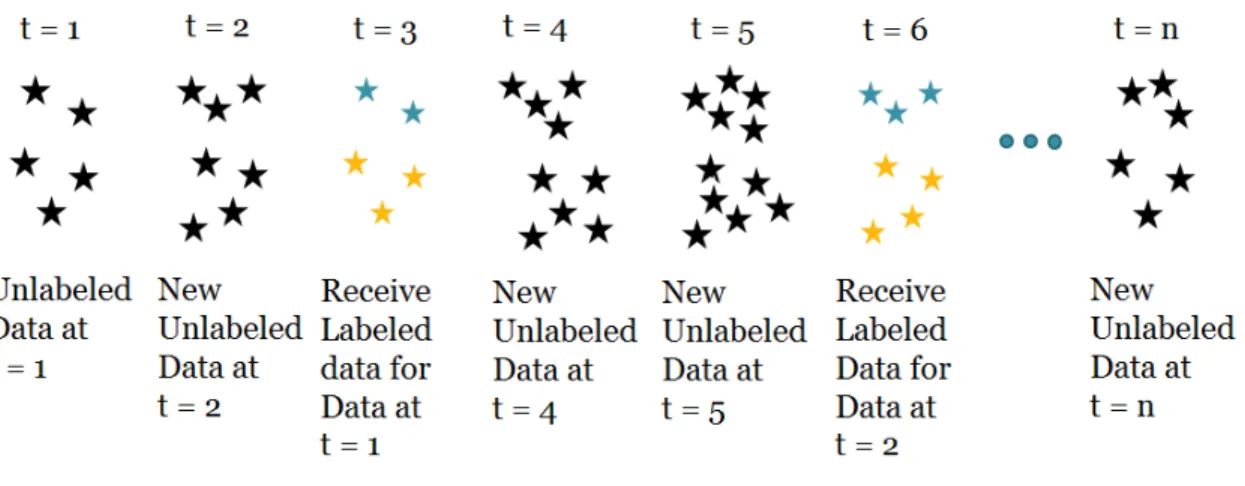
Figure 2. Graphical representation of verification latency: unlabeled data are received during first two time stepst = 1andt = 2, with labels for thet = 1data are received at
t = 3. New unlabeled data are received at t = 4andt = 5, followed by labels for data received att = 2. The process continues receiving label for data for previous timesteps in a possibly irregular intervals.
In such cases, limited amount of data may get labeled, and event then, only with a delay, and not immediately after data first becoming available. Such a scenario is referred to asverification latency, which acknowledges an additional and important constraint that must be addressed in streaming environments: labeled data may not be available at every time-step, nor even in regular intervals, which in turn significantly complicates the learning process. Verification latency, as denoted in [12], describes a scenario where true class labels are not made available until sometime after the classifier has made a prediction on the current state of the environment. The duration of this lag may not be known a priori, and may vary with time; yet, classifiers must propagate information forward until the model
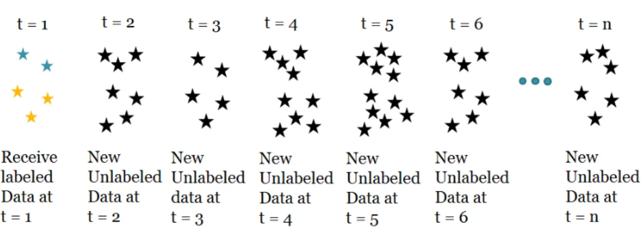
can be verified. The graphical representation of this phenomenon is shown in Figure 2. In theextreme verification latencyscenario, this lag becomes infinite, meaning that no labeled data are ever received after initialization, as illustrated in Figure 3. We call such an environment as aninitially labeled non stationary environment(ILNSE) or simply initially labeled streaming environment (ILSE) [13].
Real-world examples of such an extreme learning setting are rapidly growing be-cause of massive automated and autonomous acquisition of sensor, web user, weather, fi-nancial transaction, energy usage, and other data. Furthermore, such applications can be increasingly important. For example, network intrusion with malicious software (malware) attacks, where malware programmers are able to modify the malware faster than network security can identify and neutralize it, is a major current day challenge. Creating a labeled database for this scenario is difficult and expensive.
Figure 3. Graphical representation of extreme verification latency scenario: labeled data are received initially at t = 1; then only unlabeled data are received thereafter for t = 2,3, ...., n
Many automation applications provide other examples, such as robotic control sys-tems, drones, and autonomous vehicles. Just the recent popularization of drones opens new challenges to the computerized automation of flights of these aerial vehicles. Given a drone initially trained in a known environment, they need to incrementally adapt to changes in speed and direction of the wind, altitude, temperature, and atmospheric pressure in an unsupervised manner.
Chapter 3
Preliminary and Related Work
In this chapter, we describe in detail the algorithms currently available in the lit-erature for learning from a streaming nonstationary data in the presence of extreme ver-ification latency (EVL). As a relatively new field of machine learning, there are only a handful of algorithms that can address learning in an EVL scenario. These algorithms are Arbitrary Sub-Population Tracker (APT), Stream Classification Algorithm Guided by Clustering (SCARGC), Micro-cluster for Classification (MClassification) and Compacted Object Sample Extraction (COMPOSE).
3.1 Arbitrary Sub-Population Tracker Algorithm (APT)
The Arbitrary Sub-Population Tracker (APT) is proposed by Krempl [14] to handle extreme verification latency problem under certain assumptions and specific scenarios, and is based on the principle that each class in the data can be represented as a mixture of arbi-trarily distributed sub-populations. The APT algorithm makes the following assumptions [60]:
1. The underlying population of the feature space contains several sub-populations, each of which drifts (possibly) differently over time;
2. The data generated from this feature space can be represented with a mixture model of several drifting components;
3. Initial labeled data are used to represent each sub-population of the feature space, where a sub-population is defined as a mode in the class-conditional distribution
p(y|x), with p(y) representing the prior distribution of the class labels, and p(x) representing the marginal feature distribution;
4. A multimodal class distribution is represented by individual sub-populations to be tracked within a single class; furthermore every instance of the feature space must be labeled at the initialization;
5. The drift only affects the conditional feature distributionsp(x|z), where p(z) repre-sents the components’ prior distributions, i.e., the mixing proportions of components used in the mixture model to represent data;
6. The drift is gradual and systematic that can be represented as a piecewise linear function;
7. The conditional posterior distributionp(y|z)remains fixed, i.e., a components class label cannot change
8. The prior distribution of components,p(z), is static
9. The posterior distribution is independent of the (latent) component membership,
p(y|z) =p(y|z, x); and
10. Co-variance of each component remains constant.
Non-parametric kernel density estimation is used to estimate conditional feature distribu-tions p(x|z) of the components, using M samples, X = x1, x2, .., xM. Krempl uses the
common choice of Gaussian (radial basis) kernel for estimation, however any standard ker-nel estimator can be used for this purpose, such as the polynomial kerker-nel. The standard
kernel estimator modelingpˆ(x)is given as ˆ p(x) = 1 M M X m=1 KX(x−xm) (3.1)
where,KX(x−xm)is the kernel function. When a D-dimensional Gaussian kernel is used
as the kernel, we then have
KX(x−xm) = (2π) D 2|C−1| 1 2 exp{−1 2(x−xm) T C−1(x−xm)} (3.2)
where C is the covariance or generally referred to as bandwidth of the Gaussian kernel function.
A modification to the standard Gaussian kernel is proposed to actually model the conditional feature distributionpˆ(x|z), instead of simply modeling the feature distribution ˆ
p(x). The modified Gaussian kernel incorporates each component z of the data, allows different bandwidth matrix for each component, and also accounts for the drift present in the data. In other words, the Gaussian kernel is modified to better fit APT to work in the non-stationary environments. The adjusted kernel estimator accounting for drift present in the data is given as
ˆ p(x|z) = ˆp(x|z, t) = 1 M M X m=1 Gm(x, t) (3.3)
whereGm(x, t)is the modified Gaussian Kernel and is represented as
Gm(x, t) = (2π) D 2|C−1 zm| 1 2 exp{−1 2d T mC −1 zmdm} (3.4)
where Czm allows there to be a different bandwidth matrix for each component z, and
dm = x −(xem)(t) is the difference between position x and the estimated position xem of the mth component at time t. Here, the estimated position is computed as(xem)(t) =
xm + (t −tm)∗µ∆zm, where µ
∆
zm represents the component movement vector of the m
th
component center. The initial cluster position is indicated byµ0zm.
The learning strategy of APT is twofold; first, the optimal one-to-one assignment between labeled instances in time-stept and unlabeled instances in time-step t+ 1is de-termined using expectation maximization (EM) algorithm. The EM algorithm begins with the expectation step by predicting which instances are most likely to correspond to a given sub-population. During the maximization step, the algorithm determines which drift pa-rameters maximize the expectation. Then, the classifier is updated to reflect the population parameters of the newly received data and drift parameter relating the previous time step to the current one. Following the assumption thatp(z)remains static, the algorithm creates a one-to-one mapping of an instance in time stept to a corresponding instance in time step
t + 1. Given a set of M known examples and a set of N new observations at positions
X = x1, x2, .., xN at times T = t1, t2, .., tN, the problem corresponds to the following
likelihood maximization problem
L(Θ, X, T) = N Y n=1 M Y m=1 Gm(xn, tn)znm (3.5) whereΘ ={µ0
1, ...., µ0k, µ∆1, ...., µ∆k}, andznmis the latent instance-to-exemplar
correspon-dence, which is equal to 1 if instancencorresponds to exemplarmand 0 otherwise. Establishing a one-to-one relationship while identifying drift requires an imprac-tical assumption that the number of instances remains constant throughout all time steps. Krempl relaxes this assumption by establishing a relationship in a batch method - matching a random subset of exemplars to a subset of new observation until all new observations have been assigned a relationship to an exemplar.
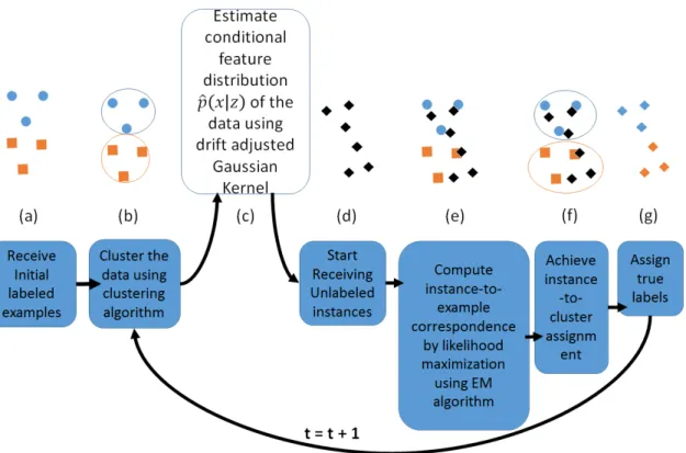
Figure 4. Block diagram and Graphical Representations of APT; (a) Receive initial labeled examples (represented by blue circles and orange rectangles), (b) Perform clustering of the data (represented by blue and orange circles around the data), (c) Estimate the conditional feature distribution of the data p(x|z) using modified Gaussian Kernel given in equation 3.3, (d) Start receiving unlabeled examples (represented by black diamonds), (e) Maximize the likelihood function given in equation 3.5 to compute instance-to-example correspon-dence, (f) Pass the same cluster assignment from the examples to its assigned instances to achieve instance-to-cluster assignment, (g) Assign same label of the example to its assigned instance.
Krempl suggests a bootstrap method that can make the one-to-one assignments more robust, but at an additional computational cost. When the assumptions are satisfied, APT works very well. However, APT has two primary weaknesses: 1) some of its assump-tions often do not hold true, causing a decrease in performance, and 2) it is computationally very expensive [13].
representation of the algorithm illustrating its corresponding stages through block diagrams is given in Figure 4.
Algorithm 1. Arbitrary Subpopulation Tracker (APT)
Inputs: Initial labeled data Dinit; A clustering algorithm with its own free
parame-ters; a suitable bandwidth matrices calculation algorithm; a suitable expectation-maximization (EM) algorithm with its free parameters
1: Receive M training examples formDinit ={xi;yi}; i = 1, ..., M ;x ∈ X;y ∈ Y =
{1, ..., c};
2: Run clustering algorithm to partition the data intoKdisjoint subsets and associate each cluster to one class amongcclasses ;
3: Estimate the conditional feature distribution of the datapˆ(x|z)using equation 3.3;
4: Receive new unlabeled instances Ut= {xtu ∈X ,u= 1, ..., N} and assume N = M
to associate each new instance to one previous example;
5: Compute instance-to-exemplar correspondence by maximizing the likelihood given in equation 3.5 using EM algorithm;
6: Pass the cluster assignment from the example to their assigned instances to achieve
instance-to-cluster assignment;
7: Pass the class of an examplexi i.e.yito the class of its assigned instance;
8: Go to step 2 and Repeat.
3.2 Stream Classification Algorithm Guided by Clustering (SCARGC)
Souza et al. proposed an alternate algorithm, SCARGC, to solve the extreme ver-ification latency problem [15]. SCARGC is a clustering-based algorithm that repeatedly clusters unlabeled input data, and then classifies the clusters using the labeled clusters from the previous time-step. SCARGC also makes several assumptions:
1. A small amount of labeled data is available initially to define the problem;
2. The drift is gradual / incremental, which allows tracking of the classes with only unlabeled information. Incremental drift assumption as used in SCARGC requires
significant overlap between class distributions in subsequent time steps and short intervals of time;
3. The number of classes is known and fixed ahead of time.
Given the aforementioned assumptions, the algorithm builds an initial classification model using the available labeled data from c classes, and then divide the initial labeled data into k ≥ c clusters where k is a user-selected free parameter. If user selects k = c, SCARGC usescclasses as initial clusters, otherwise a clustering subroutine finds clusters and associates each cluster with one class. Souza denotes this initial set of k clusters as
C0 = C0
1, C20, ., Ck0. As new unlabeled data are received, the algorithm stores each
ex-ample in a pool, and predicts its label using the initial classification model. After a fixed number of examples, also pre-determined by the user, are received and stored in the pool, the pool of examples is clustered intokclusters in the same way as initial labeled data are clustered, i.e., by usingcclasses as initial clusters ifk =c, otherwise running a clustering subroutine to associate each cluster with one class. The new set of clusters are denoted asC1 = C1
1, C21, , Ck1. Each new clusterCi1 ∈ C1 is then associated with (linked to) one
of the previous clusters C0
j ∈ C0 to assign each cluster to one class. The classification
model is updated using the recently labeled examples. The algorithm then repeats the loop, alternating between clustering and classification. The labels are decided by associating clusters Ct in the current iteration with the labels of clusters Ct−1 from the previous
it-eration. The mapping between the clusters is performed by centroid similarity between current and previous iterations using Euclidean distance. Given the current centroids from the most recent unlabeled clusters and past centroids from the previously labeled clusters,
one-nearest neighbor algorithm (or support vector machine) is used to label the centroid from current unlabeled clusters.
SCARGC is computationally efficient, but its performance is highly dependent on the clustering phase. It also requires some prior knowledge such as the number of classes and the number of modes for each class in the data, the latter of which may limit the use of this algorithm when such information is not available.
The block diagram representing different stages of SCARGC with accompanying illustrations is given in Figure 5.
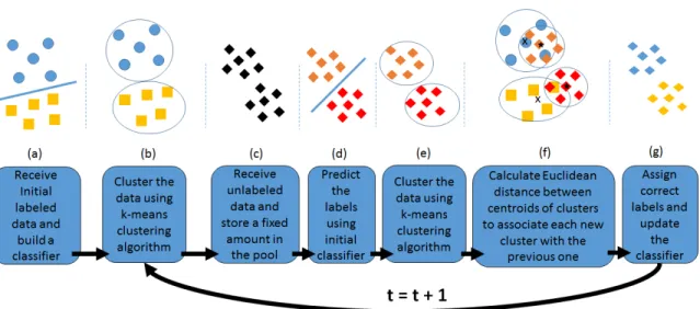
Figure 5. Block diagram and Graphical Representations of SCARGC; (a) Receive initial labeled data and classify it using 1-NN or SVM classifierφ, (b) Cluster the initial data into
k clusters to form initial clusters, (c) start receiving unlabeled examples and store them in a pool, (d) initial classifier modelφis used to predict their labels, (e) cluster the unlabeled examples labeled byφusingk-means clustering to create new clusters at current iteration, (f) Perform mapping between clusters from previous and current iteration using centroid similarity, (g) Assign correct labels to unlabeled examples and update φ. The process repeats by clustering the newly labeled data in the previous step
clas-sifierφas shown in Figure 5(a). In Figure 5(b), SCARGC clusters the data intokclusters to form initial clusters. The algorithm then receives unlabeled examples and stores them in a pool as shown in Figure 5(c), and uses the initial classifier modelφto predict their labels (Figure 5(d)). In Figure 5(e), the algorithm clusters the unlabeled examples labeled by φ
usingk-means clustering to create new clusters at current iteration. The mapping between clusters from previous and current iteration are then obtained using centroid similarity (Fig-ure 5(f)), the labels are assigned, and the classifier is updatedφ. This process continues as long as new unlabeled data are received.
The pseudocode for SCARGC algorithm is given in Algorithm 2
Algorithm 2.SCARGC
Inputs: Initial training dataDinit, maximum pool sizeN, number of clustersk;
1: Receive initial labeled dataDinit={xi;yi};i= 1, ..., M ;x∈X;y∈Y ={1, ..., c}
2: Build initial classifierφusingDinit
3: Run k-means clustering algorithm to divide the data into k clusters; {Ct =
Ct
1, C2t, ..., Ckt}and associate each cluster with one of thecclasses
4: Start receiving new unlabeled examples from unlabeled data streamU ={xu∈X}
5: Store the next batch ofN examples in a pool
6: Predict labels of stored examples using classifier φ as Dnew = {xu;φ(xu)};u =
1, ..., N
7: Runk-means clustering algorithm onDnew to obtain{Ct+1 =C1t+1, C t+1
2 , ..., C
t+1
k }
8: Establish a mapping between current and previous clusters: the current clusters Ct+1
are associated to previous clustersCtby measuring similarity between their centroids
qti;i = {1, ..., k}using Euclidean distance, i.e., Dist(qt, qt+1)whereDistrepresents
Euclidean distance
9: Assign current centroid qi
t+1 the label yˆi which is same label yi of the closest past
centroidqit
10: The current dataset now has the updated correct labels from the previous step asDt+1 =
{xu; ˆyu)};u= 1, ..., N
11: Update the initial classifierφusingDt+1
3.3 Micro-Cluster for Classification (MClassification)
Souza et al. also proposedMClassification, an algorithm that uses the idea of micro clusters (MC) [16] to adapt to the changes in the data over time, and learn the concepts under extreme verification latency. A Microcluster (MC) is a compact representation of the data pointsx~i;i = {1, ..., N}, that includes the sufficient statistics of the data and are
represented in triplets (N, ~LS, ~SS), where N is the number of data points in the cluster,
~
LSis the linear sum ofN data points represented asLS~ ={x~1+x~2+...+x~n}, andSS~
is the square sum of data points represented asSS~ ={x~12+x~22+...+x~n2}. Thus a MC
summarizes the information about the set ofN data points, from which we can calculate the centroid and radius of the MC using the following equations
centroid = LS~ N (3.6) Radius= s ~ SS N −( ~ LS N ) 2 (3.7)
There exist two interesting properties of MC, referred to asincrementality andadditivity, which make them suitable for the streaming problems. Theincrementalityproperty states that if we are given a set of data points whose statistics are stored in a micro-cluster A
as M CA = (NA,(LS~ A),(SS~ A)), we can incrementally add a new example ~x in M CA
updating the statistics of data points in the following way
(LS~ A)←(LS~ A) +~x (3.8)
(SS~ A)←(SS~ A) + (~x)2 (3.9)
whereas theadditivityproperty provides that, if we have two disjoint Micro-clustersM CA
andM CB, the union of these two groups is equal to the sum of its parts. Thus the sufficient
statistics of a new Micro-ClusterM CC = (NC,(LS~ C),(SS~ C)), that stores the information
ofM CA∪M CB are computed as:
(LS~ C)←(LS~ A) + (LS~ B) (3.11)
(SS~ C)←(SS~ A) + (SS~ B) (3.12)
NA ←NB+NC (3.13)
Although MC is efficient and appropriate for data streaming problems, the authors observe that MC representation has been commonly used in clustering problems. In order to use MC to classify evolving data streams, the authors modify the representation to store information about the class of data points, thus their representation is a 4-tuple(N, ~LS, ~SS, y), where
yis the label for a set of data points. The working of the algorithm is presented below. The algorithm begins by receiving the initial labeled data Dinit, using which it
builds a set of labeled MCs, where each MC has information about only one example. The algorithm then starts receiving the unlabeled data stream. A labelyˆt is then predicted
for each example x~t from the stream based on its nearest MC, computed with respect to
Euclidean distance in the classification phase. The examplex~tis added to its corresponding
nearest MC, sayM CN, using the incrementalityproperty of MC. Now the updated radius
of M CN is computed and the algorithm checks if the updated radius of M CN exceeds
the maximum micro-cluster radius thresholdr defined by the user. If the radius does not exceed the thresholdr, the examplex~tremains added inM CN and its updated centroid is
moved in direction of the newly emerging concept of the class for new example added. On the other hand, if the radius exceeds the threshold, a new MC sayM CN0 carrying the predicted label yˆt is created to allocate the new example x~t. The process is repeated for
each newly received unlabeled example.
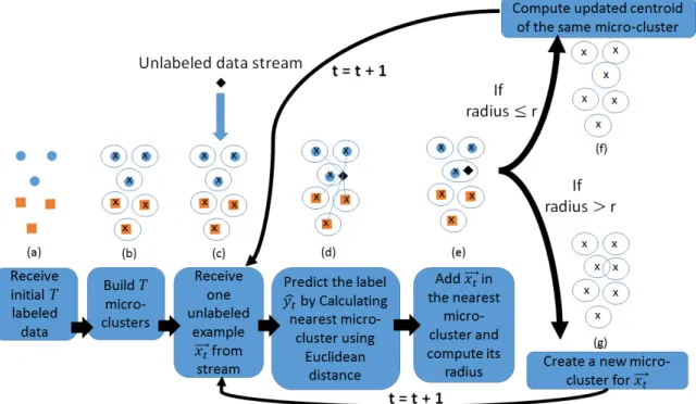
The descriptive diagram illustrating different stages of the process is given in Fig-ure 6. The pseudocode for MClassification algorithm with the implementation details is provided in Algorithm 3.
Algorithm 3.MClassification Inputs: Maximum micro-cluster radiusr;
1: Receive initial labeled dataDinit={xi;yi};i= 1, ..., T ;x∈X;y ∈Y ={1, ..., c}
2: Build T micro-clusters asM Ci = (Ni, LSi, SSi, yi);i = 1, ..., T whereN = number
of data points ;LS =PN
j=1xj ;SS=
PN
j=1(xj)2
3: Calculate sufficient statistics of each micro-cluster as follows centroidi = ~ LSi Ni;Radiusi = q ~ SSi Ni −( ~ LSi Ni ) 2
4: Receive one new unlabeled example~xtfrom the unlabeled data stream
U ={xu ∈X}
5: Measure distance between x~t and each micro-cluster centroids centroidi;i =
{1, ..., T}i.e.Dist(centroidi, ~xt)to find closest micro-cluster sayM CN, whereDist
represents the Euclidean distance
6: Assign label ofM CN i.e.yˆtto classify examplex~t
7: Add examplex~ttoM CN and compute its sufficient statisticsradiusN ; andcentroidN
8: ifradiusN > rthen
9: Create a new micro-cluster for examplex~tsayM CN0 = (N
0 N, LS 0 N, SS 0 N,yˆt) 10: else
11: Add example x~t to M CN and update its statistics as (LS~ N) ← (LS~ N) + ~
xt; (SS~ N)←(SS~ N) + (x~t)2;NN ←NN + 1
12: end if
Figure 6. Block diagram and Graphical Representations of MClassificaion; (a) Receive initial T labeled examples (represented by blue circles and orange rectangles), (b) build
T micro-clusters (represented by circles around each example) from the initial data and compute their sufficient statistics (black cross represents the centroid of a particular micro-cluster), (c) start receiving one unlabeled example ~xt (represented by a black diamond)
from the unlabeled data stream, (d) compute nearest micro-cluster from~xtusing Euclidean
distance, (e) Add ~xt in the nearest micro-cluster and calculate its updated radius, (f) If
radius does not exceed the threshold radiusr, update the sufficient statistics of the same micro-cluster and also compute its updated centroid which will be slightly dislocated to-wards the new concept, (g) If radius exceeds the threshold radius r, create new micro-cluster for~xtand update its corresponding statistics.
3.4 COMPOSE.V1 (Original COMPOSE Withα-Shape Construction)
TheCOMPactedObjectSampleExtraction (COMPOSE) framework is introduced in [13] to address the extreme verification latency problem in an ILSE setting, i.e., learn drifting concepts from a streaming non stationary environment that provides only unlabeled data after initialization. The algorithm only makes an assumption of gradual/limited drift in