Interventional effects for mediation analysis with multiple mediators.

(1)

Vansteelandt, S; Daniel, RM (2016) Interventional effects for me-diation analysis with multiple mediators. Epidemiology (Cambridge,

Mass). ISSN 1044-3983 DOI: https://doi.org/10.1097/EDE.0000000000000596

Downloaded from: http://researchonline.lshtm.ac.uk/3199919/

DOI:10.1097/EDE.0000000000000596

Usage Guidelines

Please refer to usage guidelines at http://researchonline.lshtm.ac.uk/policies.html or alterna-tively [email protected].

(2)

Interventional e

↵

ects for mediation analysis with

multiple mediators

Stijn Vansteelandt

Department of Applied Mathematics, Computer Sciences and Statistics

Ghent University, Belgium

and Rhian Daniel

Department of Medical Statistics and Centre for Statistical Methodology

London School of Hygiene and Tropical Medicine, U.K.

The mediation formula for the identification of natural (in)direct e↵ects has facilitated mediation analyses that better respect the nature of the data, with greater consideration of the need for confounding control. The default assumptions on which it relies are strong, however. In particular, they are known to be violated when confounders of the mediator-outcome association are a↵ected by the exposure. This complicates extensions of counterfactual-based mediation analysis to settings that involve repeatedly measured mediators, or multiple correlated mediators.

VanderWeele, Vansteelandt and Robins introduced so-called interventional (in)direct e↵ects. These can be identified under much weaker conditions than natural (in)direct e↵ects, but have the drawback of not adding up to the total e↵ect. In this article, we adapt their proposal in order to achieve an exact decomposition of the total e↵ect, and extend it to the multiple mediator setting. Interestingly, the proposed e↵ects capture the path-specific e↵ects of an exposure on an outcome that are mediated by distinct mediators, even when – as often – the structural dependence between the multiple mediators is unknown; for instance, when the direction of the causal e↵ects between the mediators is unknown, or there may be unmeasured common causes of the mediators.

(3)

Running head: Interventional e↵ects for multiple mediation analysis.

Corresponding author: Stijn Vansteelandt, Ghent University, Department of Applied Mathematics, Computer Science and Statistics, Krijgslaan 281, S9, 9000 Gent, Belgium email: [email protected], tel: ++32 9 2644776

(4)

Interventional e

↵

ects for mediation analysis with

multiple mediators

March 22, 2016

The mediation formula for the identification of natural (in)direct e↵ects has facilitated mediation analyses that better respect the nature of the data, with greater consideration of the need for confounding control. The default assumptions on which it relies are strong, however. In particular, they are known to be violated when confounders of the mediator-outcome association are a↵ected by the exposure. This complicates extensions of counterfactual-based mediation analysis to settings that involve repeatedly measured mediators, or multiple correlated mediators.

VanderWeele, Vansteelandt and Robins1 _{introduced so-called interventional (in)direct} e↵ects. These can be identified under much weaker conditions than natural (in)direct e↵ects, but have the drawback of not adding up to the total e↵ect. In this article, we adapt their proposal in order to achieve an exact decomposition of the total e↵ect, and extend it to the multiple mediator setting. Interestingly, the proposed e↵ects capture the path-specific e↵ects of an exposure on an outcome that are mediated by distinct mediators, even when – as often – the structural dependence between the multiple mediators is unknown; for instance, when the direction of the causal e↵ects between the mediators is unknown, or there may be unmeasured common causes of the mediators.

1 Introduction

The introduction of counterfactual-based distribution-free definitions of direct and indi-rect e↵ect in epidemiology2,3 _{– so-called natural (in)direct e↵ects – has spurred a major} revival of mediation analysis4–6_{. It has led to a renewed and improved understanding of} the ignorability assumptions required to identify (in)direct e↵ects. It has moreover en-abled the development of a formal framework for mediation analysis that is applicable to nonlinear models. These developments have facilitated applications of mediation analysis that better respect the nature of the data and reflect greater consideration of the need for confounding control. Notwithstanding this, mediation analysis based on natural (in)direct e↵ects has been the subject of recent critiques. The usefulness of natural (in)direct e↵ects

(5)

has been called into question because they are not directly informative about real-life interventions7,8_{. Concerns have moreover been raised about the impossibility to} con-duct experiments in which the identification assumptions for natural (in)direct e↵ects are guaranteed to be satisfied7,9,10_{. Remaining concerns arise from the difficulty or} impossi-bility to identify these e↵ects in realistic settings that involve multiple and/or repeatedly measured mediators11–13_{, and settings that involve exposure-induced confounding of the} mediator-outcome association1,14,15_{. These concerns all originate from the fact that} nat-ural (in)direct e↵ects are defined in terms of so-called cross-world counterfactuals7 _that are unobservable, even from experimental data; they call for alternative e↵ect measures that are less remote from the observed data.

In this article, we revisit and refine so-called interventional (in)direct e↵ects, previously introduced by VanderWeele, Vansteelandt and Robins1_{. These are not defined in terms} of cross-world counterfactuals. They can therefore be identified under weaker conditions, but have the drawback of not always adding up to the total e↵ect. We will adapt this proposal to overcome this, and next extend it to the case of multiple mediators. Inter-estingly, our proposal decomposes the total e↵ect into di↵erent path-specific e↵ects via the di↵erent mediators, even when – as often – the structural dependence between the multiple mediators (for instance, the direction of the causal e↵ect, or the possible presence of unmeasured common causes) is unknown. It thus opens avenues towards a flexible and realistic mediation analysis with multiple mediators.

2 Single mediator models

2.1 E

↵

ect measures

Let A, M and Y denote the exposure, mediator and outcome. Let C represent baseline covariates not a↵ected by the exposure. We letYa and Ma denote respectively the values

of the outcome and mediator that would have been observed had the exposureAbeen set to level a; let Yam denote the value of the outcome that would have been observed had

A been set to levela, and M to m. Throughout, we make the consistency assumption16 that Ya=Y and Ma=Y whenA=a, and that Yam =Y when A= aand M =m.

Suppose a and a⇤ are two values of the exposure we wish to compare, e.g. a = 1 and

a⇤ _{= 0. The corresponding average controlled direct e↵ect, fixing the mediator to level}

m, is then defined byE(Yam Ya⇤_m). It captures the e↵ect of exposure Aon outcomeY, intervening to fixM tom2,4_{; it may be di↵erent for di↵erent levels of}_m_{. The natural direct} e↵ect,E(YaMa⇤ Ya⇤Ma⇤), di↵ers from the controlled direct e↵ect in that the intermediate

M is set to the levelMa⇤, the level that it would have naturally been under some reference

condition a⇤ _{for the exposure}2,4_{. By subtracting it from the total e↵ect,}_E₍_Y

a Ya⇤), one

obtains the average natural indirect e↵ect,E(YaMa YaMa⇤); this compares the e↵ect of the mediator at levelsMaandMa⇤on the outcome when exposure is set toA=a. Finally,

(6)

we define the interventional direct e↵ect as E⇣YaGa⇤|C Ya⇤Ga⇤|C ⌘ =E " X m {E(Yam|C) E(Ya⇤_m|C)}P(M_a⇤ =m|C) # .

It di↵ers from the controlled direct e↵ect in that the intermediate is set for each subject to a random draw from the conditional distribution of Ma⇤, given the observed covariates

C for that subject (a related definition1 _uses_P₍_M ₌_m_|_a⇤_{, C}_{) in lieu of}_P₍_M

a⇤ =m|C)). It may thus be viewed as the controlled direct e↵ect of comparing exposure levelsaversus

a⇤ under a stochastic intervention, Ga⇤_|_C, which controls the mediator for each subject at some value randomly drawn from the distribution of Ma⇤, given the observed covariates

C. We will moreover call

E⇣YaGa|C YaGa⇤|C ⌘ =E " X m E(Yam|C){P(Ma=m|C) P(Ma⇤ =m|C)} #

the interventional indirect e↵ect. For this e↵ect to be non-zero, the exposure would have to change the mediator, which in turn would have to change the outcome, thus confirming that it captures a notion of mediation. For instance, VanderWeele et al.17 _investigate pack-years of smoking as a mediator of the e↵ect of genetic variants on lung cancer. The interventional indirect e↵ect expresses the change in lung cancer risk that would be seen if the distribution of pack-years of smoking were shifted from what it would be if all subjects carried two risk alleles to what it would otherwise be. Arguably, this e↵ect is more relevant than the corresponding natural indirect e↵ect, as it is informative about the e↵ect of particular interventions on smoking. One could alternatively define interventional (in)direct e↵ects with respect to a mediator distribution other than P(Ma= m|c). This

can be of interest when interventions on the exposure are not conceivable. For instance, changingP(Ma=m|c) toP(M =m|a, c) would change the interpretation to the average

change in lung cancer risk that would be seen if the distribution of pack-years of smoking were shifted from what it is in subjects with two risk alleles to what it is in the remaining subjects1_{. In the remainder of the article, we choose not to do this because unmeasured} confounding may renderP(M = m|a, c) dependent on a, even when the exposure has no e↵ect on the mediator.

2.2 Assumptions

Controlled direct e↵ects can be identified when:

(i) the e↵ect of exposure A on outcome Y is unconfounded conditional on C (i.e., Yam

??A|C, where X ??Y|Z denotes thatX is independent ofY conditional on Z);

(ii) the e↵ect of mediator M on outcome Y is unconfounded conditional on A, C and possibly some additional covariate vectorLthat may be a↵ected by A(i.e., Yam ??

(7)

Average interventional (in)direct e↵ects are identified if, in addition to these assumptions,

(iii) the e↵ect of exposure A on mediator M is unconfounded conditional on C (i.e.,

Ma?? A|C).

Randomisation of the exposure (possibly conditional on C) ensures the validity of this additional assumption as well as assumption (i). Under (i)-(iii), the interventional direct and indirect e↵ect can be identified as1

X c X l X m {E(Y_|a, l, m, c)P(l_|a, c) E(Y_|a⇤, l, m, c)P(l_|a⇤, c)_}P(m_|a⇤, c)P(c)(1) X c X l X m E(Y_|a, l, m, c)P(l_|a, c)_{P(m_|a, c) P(m_|a⇤, c)_}P(c). (2) These expressions reveal a major weakness that we will attempt to overcome: the sum of the e↵ects (1) and (2), which is sometimes called the ‘overall e↵ect’1_{, may di↵er from} the total e↵ect. One exception is when assumptions (i) and (iii) hold, and in addition, assumption (ii) holds with L empty. In that case, the direct and indirect interventional e↵ects sum to the total e↵ect E(Ya Ya⇤), even when there are interactions and

non-linearities.

Natural direct and indirect e↵ects always sum to the total e↵ect. However, their iden-tification requires much stronger assumptions. It requires that assumptions (i) and (iii) hold, that assumption (ii) holds with L empty (thus excluding the possible presence of exposure-induced confounders), and in addition that a technical cross-world independence assumption3 _{holds, which places an independence restriction on the joint distribution of} the variables Yam and Ma⇤:

(iv) Yam ??Ma⇤|C.

Under these assumptions, these e↵ects reduce to expressions (1) and (2) obtained for average direct and indirect interventional e↵ects, but with Lempty. It thus follows that in single mediator models without post-treatment confounding, natural (in)direct e↵ects obtained under assumption (iv) can also be interpreted as interventional (in)direct e↵ects (even when that assumption is violated).

2.3 Natural versus interventional (in)direct e

↵

ects

Average interventional direct e↵ects encode the exposure e↵ect that would be realised while controlling the mediator distribution to be fixed. This is realised by setting the mediator for each subject to a random draw from the distribution of the mediator at exposure level a⇤_{, given covariate values} _c_{. Natural direct e↵ects adopt a similar notion,}

but fixing the mediator at the counterfactual mediator value (corresponding to exposure level a⇤_{) itself. This may yield a direct e↵ect of a di↵erent magnitude, in part because}

(8)

the counterfactual level of the mediator may depend on much more than the considered covariates c. Both measures would thus be relatively close if the covariate set c were so rich as to leave little variation in Ma⇤ for a given c (beyond the variation due to causes unrelated toYam), but not necessarily otherwise. While the natural direct e↵ect may thus

more closely capture the notion of mechanism, this need not lead us to prioritise them. First, natural direct e↵ects employ cross-world counterfactuals like YaMa⇤ about which information cannot be obtained even from experimental data. The data analyst who reports natural direct e↵ects is thus obligated to make strong untestable assumptions like (iv) (and/or to conduct a sensitivity analysis18_{), under which these e↵ects reduce to the} interventional direct e↵ect (1) (withLempty). Second, the relevance of natural (in)direct e↵ects has been questioned on the basis that they do not connect to the e↵ect of particular policies8_.

In contrast to natural (in)direct e↵ects, interventional (in)direct e↵ects are policy-relevant19_{: they are relevant about a policy that involves fixing the mediator distribution,} or shifting it to the extent that it is a↵ected by the exposure. They continue to be mean-ingful, even when assumptions (i) and (iii) fail or when the exposure is not manipulable (e.g. when the exposure is race20_{), so long as assumption (ii) is satisfied. For instance,} when Lis empty, then the interventional direct e↵ect (1) reduces to

X

c

X

m

{E(Ym|a, c) E(Ym|a⇤, c)}P(m|a⇤, c)P(c),

since E(Y_|a, m, c) = E(Ym|a, c) under assumption (ii). This can be interpreted as the

average outcome di↵erence that would remain between exposure groupsA=aandA= a⇤

if the mediator distribution in the former group were shifted to equal that in the latter group20_{. Similar comments are relevant for indirect e↵ects.}

3 Multiple mediator models

3.1 Review

For pedagogic purposes, we consider a setting with two mediators M1 and M2, and fer more general results to the eAppendix. VanderWeele and Vansteelandt (2013) de-fine the natural direct e↵ect of A on Y, not mediated by either or both mediators, as

E(YaM1a⇤M2a⇤ Ya⇤M1a⇤M2a⇤). The remaining indirect e↵ect via both mediators is then

E(YaM1aM2a YaM1a⇤M2a⇤). These e↵ects can be identified as X c X m1 X m2 {E(Y|a, m1, m2, c) E(Y|a⇤, m1, m2, c)}P(m1, m2|a⇤, c)P(c) (3) and _X c X m1 X m2 E(Y_|a, m1, m2, c){P(m1, m2|a, c) P(m1, m2|a⇤, c)}P(c), (4)

(9)

when

(i’) the e↵ect of exposure A on outcome Y is unconfounded conditional on C (i.e.,

Yam1m2 ??A|C);

(ii’) the e↵ect of both mediators M1 andM2 on outcome Y is unconfounded conditional onA and C (i.e., Yam1m2 ??(M1, M2)|{A=a, C});

(iii’) the e↵ect of exposure A on both mediators is unconfounded conditional onC (i.e., (M1a, M2a)?? A|C);

(iv’) the cross-world assumption holds that Yam1m2 ??(M1a⇤, M2a⇤)|C.

Unfortunately, these e↵ects provide no insight into the distinct pathways that may exist between exposure and outcome.

When the mediators are sequential (i.e., M1 may a↵ectM2 but not vice versa), further progress1,12 _{can sometimes be made by supplementing the previous analysis with a single} mediator analysis with respect toM1. In particular, if assumptions (i)-(iv) hold withM1 in lieu of M, one can additionally identify the natural direct e↵ect E(YaM1a⇤ Ya⇤_M₁_a⇤). This can be decomposed as

E(YaM1a⇤ YaM1a⇤M2a⇤) +E(YaM1a⇤M2a⇤ Ya⇤M1a⇤M2a⇤),

where the first component represents the e↵ect mediated by M2 but not M1, and the second component can be identified as detailed in the previous paragraph. Such sequential analysis thus enables one to infer the direct e↵ect that is not mediated by either M1 or

M2 or both, i.e. E(YaM1a⇤M2a⇤ Ya⇤M1a⇤M2a⇤), the e↵ect that is mediated by M1, i.e.

E(YaM1a YaM1a⇤) (including any e↵ect mediated by both M1 and M2), and the e↵ect that is mediated byM2 but not M1, i.e.E(YaM1a⇤ YaM1a⇤M2a⇤). However, one important limitation is that the causal structure between M1 and M2 (i.e. whether M1 a↵ects M2, or vice versa) is often not known when di↵erent mediators are assessed at the same time. Moreover, even when assumptions (i’)-(iv’) hold, assumptions (i)-(iv) (with M1 in lieu of

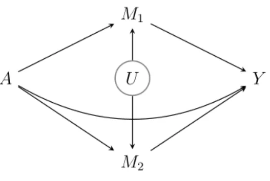
M) will often not be satisfied12_{. For instance, when both mediators share an unmeasured} common cause, as in the causal diagram of Figure 1, then M2 confounds the association between M1 and Y, thereby inducing a violation of assumption (ii). In that case, the e↵ect mediated viaM1 is not identified because the data carry no information about the e↵ect of M1 onM2. Regression adjustment forM2 provides no remedy because M2 is an exposure-induced confounder so that adjusting for it would violate assumption (iv). This problem is important because the mediators are strongly related in many applications; for instanceM1 and M2 may represent realisations of a repeatedly measured mediator, or be manifestations of an underlying latent process.

In view of these limitations, we will next propose novel definitions of interventional (in)direct e↵ects for the multiple mediator setting, which do not have the disadvantage

(10)

that they do not sum to the total e↵ect. The proposed formalism will decompose the total e↵ect of exposure on outcome into various path-specific e↵ects. It can be used even when the causal structure between the mediators is unknown or when various mediators share unmeasured common causes.

3.2 Proposal

We define the interventional direct e↵ect of exposure on outcome other than via the given mediators as E " X m1 X m2 {E(Yam1m2|c) E(Ya⇤m1m2|c)}P(M1a⇤ =m1, M2a⇤ =m2|c) # . (5) This expresses the exposure e↵ect when fixing the joint distribution of both mediators (by controlling the mediators for each subject at a random draw from their counterfactual joint distribution with the exposure set at a⇤_{, given covariates} _C_{). This corresponds to}

the e↵ectA_!Y in the causal diagrams of Figures 1, 2 and 3.

We define the interventional indirect e↵ect of exposure on outcome via M1 as

E " X m1 X m2 E(Yam1m2|c){P(M1a= m1|c) P(M1a⇤ =m1|c)}P(M2a⇤ =m2|c) # . (6) This expresses the e↵ect of shifting the distribution of mediator M1 from the counter-factual distribution (given covariates) at exposure level a⇤ _{to that at level}_a_{, while fixing}

the exposure ataand the mediatorM2 to a random subject-specific draw from the coun-terfactual distribution (given covariates) at level a⇤ _{for all subjects. The latter is chosen}

independently ofM1, so as to avoid assumptions on the joint distribution of the counter-factuals M1a and M2a⇤ corresponding to di↵erent exposure levels.

The e↵ect (6) corresponds to the e↵ectA!M1 !Y in the causal diagrams of Figures 1 and 2, and to the combination of the e↵ects A ! M1 ! Y and A ! M2 ! M1 ! Y in Figure 3. The latter can be seen upon noting that the di↵erence P(M1a = m1|c)

P(M1a⇤ = m₁|c) encodes the combination of the e↵ects A ! M₁ and A ! M₂ ! M₁. The interventional indirect e↵ect of exposure on outcome viaM1 thus captures all of the exposure e↵ect that is mediated byM1, but not by causal descendants ofM1 in the graph. Interestingly, this interpretation holds regardless of the underlying causal structure.

We define the interventional indirect e↵ect of exposure on outcome viaM2 similarly as

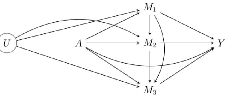
E " X m1 X m2 E(Yam1m2|c){P(M2a =m2|c) P(M2a⇤ =m2|c)}P(M1a=m1|c) # . (7) This corresponds to the e↵ect A ! M2 ! Y in the causal diagrams of Figures 1 and 3, and to the combination of the e↵ects A ! M2 ! Y and A ! M1 ! M2 ! Y in

(11)

Figure 2. It thus captures all of the exposure e↵ect that is mediated by M2, but not by causal descendants of M2 in the graph; again, this interpretation holds regardless of the underlying causal structure.

The di↵erence between the total e↵ect and these 3 e↵ects equals

E " X m1 X m2 E(Yam1m2|c){P(M1a =m1, M2a=m2|c) P(M1a=m1|c)P(M2a =m2|c) P(M1a⇤ =m₁, M₂_a⇤ =m₂|c) +P(M₁_a⇤ =m₁|c)P(M₂_a⇤ =m₂|c)}]. (8) This captures the indirect e↵ect resulting from the e↵ect of exposure on the dependence between the counterfactualsM1aand M2a, givenC. This e↵ect would be zero when both

mediators are conditionally independent21_{, given exposure and covariates, but also under} much weaker conditions. Under linear models, for instance, this e↵ect can only be non-zero when both mediators interact in their e↵ect on the outcome and, moreover, one of the mediators interacts with the exposure in its e↵ect on the other mediator. Because of this, we would often expect (8) to be much closer to zero than the other components (6) and (7) of the indirect e↵ect, though not always (see Section 4).

In some cases, the e↵ect (8) may be of primary scientific interest. For instance, consider the mediating roles of cancer stage at diagnosis and treatment in the e↵ect of SES on 1-year survival in breast cancer patients. Suppose that the treatment decision process takes cancer stage into account in a manner that may be di↵erent for women with high versus low SES. The resulting e↵ect of SES on 1-year survival that is mediated by this possibly di↵erential decision process is encoded in (8).

Regardless of whether the component (8) is of scientific interest, it is important to consider it when expressing how much of the exposure e↵ect is explained by specific pathways. For instance, in utero tobacco smoke exposure M1 is known to have an e↵ect on asthma and wheeze only in children with the GSTM1-null genotype M222. If an intervention to reduce smoking during pregnancy were only e↵ective in mothers of infants without the GSTM1-null genotype, then the intervention would have no indirect e↵ect via smoking. Yet, the indirect e↵ect (6) would be non-zero because it would consider the characteristics M1 and M2 independently. Only by acknowledging that part of the indirect e↵ect via M1 is also expressed by the term (8) may valid conclusions be drawn.

3.3 Estimation

Under assumptions (i’), (ii’) and (iii’), the e↵ects (5), (6), (7) and (8) can be identified upon substituting E(Yam1m2|c) byE(Y|a, m1, m2, c) and P(Mja =mj|c) for j = 1,2 by

P(Mj = mj|a, c) in the above expressions. Suppose for instance that the outcome obeys

model

(12)

and that the mediators (M1, M2), conditional onA and C, have means

E(Mj|a, c) = 0j+ 1ja+ 2jc,

with residual variances 2

j, j = 1,2, and covariance 12. Then the interventional direct e↵ect (5) is given by

E[_{✓1+✓5( 01+ 11a⇤+ 21C) +✓6( 02+ 12a⇤+ 22C)}(a a⇤)]

={✓1+✓5( 01+ 11a⇤+ 21E(C)) +✓6( 02+ 12a⇤+ 22E(C))}(a a⇤). It equals ✓1(a a⇤) in the absence of exposure-mediator interactions. Upon fitting the appropriate regression models to the observed data, thus obtaining estimates of the above parameters, these estimates can be plugged in to the expression above to obtain an es-timate of the interventional direct e↵ect. The interventional indirect e↵ect (6) via M1 equals

{✓2+✓4( 02+ 12a⇤+ 22E(C)) +✓5a} 11(a a⇤),

which is ✓2 11(a a⇤) in the absence of exposure-mediator and mediator-mediator inter-actions. The interventional indirect e↵ect (7) via M2 is

{✓3+✓4( 01+ 11a+ 21E(C)) +✓6a} 12(a a⇤).

Finally, the indirect e↵ect (8) resulting from the e↵ect of exposure on the mediators’ dependence is✓4 12 ✓4 12 = 0. The total e↵ect can thus be decomposed into the direct e↵ect and the two indirect e↵ects defined above. If instead, Aand M1 interacted in their e↵ect onM2 in the sense that

E(M2|m1, a, c) = 02+ 12a+ 22c+ 32m1+ 42am1, then (8) would evaluate to 2

1✓4 42(a a⇤).

This regression approach has the drawback that it requires a new derivation each time a di↵erent outcome or mediator model is considered. This can be remedied via a Monte-Carlo approach, which involves sampling counterfactual values of the mediators from their respective distributions. For instance, to evaluate the first component

E " X m1 X m2 E(Yam1m2|c)P(M1a=m1|c)P(M2a⇤ =m2|c) # ,

of (6), one may take a random drawM2a⇤_,ifor each subjectifrom the (fitted) distribution

P(M2|a⇤, ci). Next, one takes a random draw M1a,i for each subject i from the (fitted)

distribution P(M1|a, ci). Finally, one may predict the outcome as the expected outcome

under a suitable model with exposure set to a, M1 set to M1a,i, M2 set to M2a⇤_,i, and covariate Ci. The average of these fitted values across subjects then estimates the above

component. Its performance can be improved by repeating the random sampling many times and averaging the results across the di↵erent Monte-Carlo runs. In practice, we recommend the bootstrap for inference.

(13)

4 A health disparity analysis

We illustrate our proposal using data for all 29,580 women diagnosed with malignant, invasive breast cancer from 2000 to 2006 in the Northern and Yorkshire Cancer Registry Information Service (NYCRIS) – a population-based cancer registry covering 12% of the English population – who have information on cancer stage at diagnosis recorded. Our aim is to investigate possible explanations for the disparity in breast cancer survival between women of higher and lower SES; 95.9% (64.7%) of women with higher SES survive to one (five) year(s) after diagnosis, compared with 93.2% (54.1%) in the lower SES group. One possible explanation is that women with lower SES are less likely to attend screening and as a result, are more likely to be diagnosed when the disease is already more advanced. A di↵erence in treatment choice is another possible explanation.

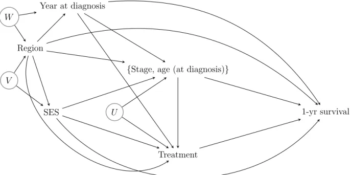
Our analyses are included mainly for illustration and some caution is warranted, as they involve several simplifications . In particular, we consider a binary SES exposure (A) which is whether or not the woman resides (at diagnosis) in an a✏uent area. The mediator M1 comprises age at diagnosis and cancer stage at diagnosis, classified as early (TNM stage 1/2) or advanced (TNM stage 3/4). The mediatorM2 is a treatment variable that classifies women either as having ‘major surgery’ or ‘minor or no surgery’. The outcome (Y) is one-year survival from the date of diagnosis. Calendar year at diagnosis and region are considered as baseline confounders (C).

All analyses assume that the causal diagram of Figure 4 holds, and are based on 6 million Monte-Carlo draws in total (to ensure that the results were free of Monte-Carlo error to the number of decimal places given), with the distribution of the two confounders equal to their empirical distribution. Standard errors are obtained using the nonparametric bootstrap, with 1,000 bootstrap samples. Stata code is given in eAppendix D.

4.1 Sequential mediation analysis

Details on the sequential mediation analysis of Section 3.1 are given in the eAppendix. The results in Table 1 suggest that, of the 2.8% (95% CI 2.3%–3.4%) total di↵erence in survival probability, about half of this (1.4%, 95%CI 1.1%–1.6%) is mediated by some combination of age and stage at diagnosis and treatment. Assuming that there are no unmeasured common causes of age/stage at diagnosis and treatment (i.e. noU in Figure 4), we can further decompose this indirect e↵ect into an e↵ect through age/stage (some of which may also act through treatment) (1.0%, 95% CI 0.8%–1.2%) and an e↵ect through treatment alone (0.3%, 95% CI 0.2%–0.5%), thus indicating that only a small proportion of the e↵ect is through the treatment variable alone.

(14)

4.2 Multiple mediator analysis based on interventional e

↵

ects

Without relying on any cross-world assumptions nor any assumptions about the causal structure of the mediators, thus allowingU in Figure 4, the results in Table 2 (obtained as detailed in the eAppendix) suggest that, of the 2.8% (95% CI 2.3%–3.4%) total di↵erence in survival probability, about a quarter of this (0.7%, 95%CI 0.5%–0.9%) is mediated by the dependence of treatment on stage and age at diagnosis, i.e. (8). Recall that we expected this e↵ect to be small, except when there are particular interactions present, as is the case here (see eTable 2). Among women of a lower SES, there is a strong negative association between stage and treatment, meaning that those diagnosed at an advanced stage are less likely to receive major surgery. One possible interpretation would be that doctors and/or patients decide that treatment is not likely to be beneficial for patients with advanced disease, or that surgical treatment is substantially delayed for these patients due to tumor-reducing treatments such as chemotherapy being prioritised first. We see from eTable 2 that this negative association is much less pronounced for women of higher SES. Therefore, we would interpret this estimated 0.7% as the increase in survival that would be expected if the treatment decision, as a function of stage and age at diagnosis (and baseline confounders), would be made for poorer women as it is currently made for higher SES women. There is little evidence of further mediation through the treatment variable (estimated e↵ect 0.02%, 95% CI: –0.05, 0.08%), and evidence of an e↵ect through age and stage at diagnosis (estimated e↵ect 0.7%, 95%CI 0.5%–0.8%). This would suggest that an additional 0.7% reduction in one-year mortality for lower SES women could be achieved if the distribution of age and stage at diagnosis (given year of diagnosis and region) were changed from that seen in lower SES women to that of higher SES women, a change that could perhaps be a↵ected by encouraging better uptake of screening and other health-seeking behaviour among lower SES women.

5 Conclusions

Most mediation analyses involve multiple mediators, either because of scientific interest in multiple pathways, or because certain confounders are mediators at the same time. When the mediators are independent21 _{or can be causally ordered}12_{, but share no (unmeasured)} common causes, then distinct pathways via those mediators can be identified. We have shown that progress can be made even in the likely event that mediators share unmea-sured common causes, or when the direction of causality is unknown. This is possible by redirecting the focus on less ambitious interventional (in)direct e↵ects. In this article, we have focused on e↵ects defined on the additive scale. We refer to eAppendix A for similar result for e↵ects on other (e.g. multiplicative) scales.

The proposed e↵ect decomposition is relatively easy to perform via a (Monte-Carlo based) regression approach. It delivers e↵ects mediated via each of the mediators sepa-rately, but also via the mediators’ dependence.

(15)

References

VanderWeele TJ, Vansteelandt S, Robins JM. E↵ect decomposition in the presence of an exposure-induced mediator-outcome confounder. Epidemiology. 2014;25:300–6. Robins JM, Greenland S. Identifiability and exchangeability for direct and indirect e↵ects.

Epidemiology. 1992;3:143–55.

Pearl J. Direct and indirect e↵ects. In: Proceedings of the Seventeenth Conference on Uncertainty and Artificial Intelligence. San Francisco: Morgan Kaufmann; 2001. p. 411–420.

VanderWeele TJ, Vansteelandt S. Conceptual issues concerning mediation, interventions and composition. Statistics and its Interface. 2009;2:457–468.

Vanderweele TJ, Vansteelandt S. Odds ratios for mediation analysis for a dichotomous outcome. Am J Epidemiol. 2010;172:1339–48.

Imai K, Keele L, Tingley D. A general approach to causal mediation analysis. Psychol Methods. 2010;15:309–34.

Robins JM, Richardson TS. Alternative graphical causal models and the identification of direct e↵ects. In: Shrout PE, Keyes KM, Ornstein K, editors. Causality and psychopathology. Oxford: Oxford University Press; 2011. .

Naimi AI, Kaufman JS, MacLehose RF. Mediation misgivings: ambiguous clinical and public health interpretations of natural direct and indirect e↵ects. Int J Epidemiol. 2014;43:1656–61.

Didelez V, Dawid AP, Geneletti S. Direct and indirect e↵ects of sequential treatments. In: Proceedings of the 22nd Annual Conference on Uncertainty in Artificial Intelligence; 2006. p. 138–146.

Imai K, Tingley D, Yamamoto T. Experimental designs for identifying causal mechanisms. Journal of the Royal Statistical Society: Series A (Statistics in Society). 2013;176:5– 51.

Imai K, Yamamoto T. Identification and Sensitivity Analysis for Multiple Causal Mechanisms: Revisiting Evidence from Framing Experiments. Political Analysis. 2013;21:141–171.

VanderWeele T, Vansteelandt S. Mediation Analysis with Multiple Mediators. Epidemi-ologic Methods. 2013;2:95–115.

Daniel RM, De Stavola BL, Cousens SN, Vansteelandt S. Causal mediation analysis with multiple mediators. Biometrics. 2015;71:1–14.

(16)

Avin C, Shpitser I, Pearl J. Identifiability of path-specific e↵ects. In: Proceedings of the International Joint Conferences on Artificial Intelligence; 2005. p. 357–363.

Vansteelandt S, VanderWeele TJ. Natural direct and indirect e↵ects on the exposed: e↵ect decomposition under weaker assumptions. Biometrics. 2012;68:1019–27. VanderWeele TJ. Concerning the consistency assumption in causal inference.

Epidemiol-ogy. 2009;20:880–3.

VanderWeele TJ, Asomaning K, Tchetgen Tchetgen EJ, Han Y, Spitz MR, Shete S, et al. Genetic variants on 15q25.1, smoking and lung cancer: an assessment of mediation and interaction. American Journal of Epidemiology. 2012;175:1013–1020.

Tchetgen Tchetgen EJ, Phiri K. Bounds for pure direct e↵ect. Epidemiology. 2014;25:775– 6.

VanderWeele TJ. Policy-relevant proportions for direct e↵ects. Epidemiology. 2013;24:175–6.

VanderWeele TJ, Robinson WR. On the causal interpretation of race in regressions adjusting for confounding and mediating variables. Epidemiology. 2014;25:473–84. Lange T, Rasmussen M, Thygesen LC. Assessing natural direct and indirect e↵ects

through multiple pathways. Am J Epidemiol. 2014;179:513–8.

Thomas D. Gene–environment-wide association studies: emerging approaches. Nat Rev Genet. 2010;11:259–72.

(17)

E↵ect Interpretation Estimate Bootstrap 95% CI SE lower upper

E(Y1 Y0) Total causal e↵ect 0.028 0.0028 0.023 0.034

E(Y1M10M20 Y0M10M20) Direct e↵ect not through{M1, M2} 0.013 0.0028 0.008 0.018

E(Y1M11M21 Y1M10M20) Indirect e↵ect through{M1, M2} 0.014 0.0014 0.011 0.016

E(Y1M10 Y0M10) Direct e↵ect not throughM1 0.017 0.0028 0.011 0.022

E(Y1M11 Y1M10) Indirect e↵ect throughM1 0.010 0.0011 0.008 0.012

E(Y1M10 Y1M10M20) Indirect e↵ect throughM2 only 0.003 0.0008 0.002 0.005

Table 1: Results of sequential mediation analysis

E↵ect Estimate Bootstrap 95% CI

SE lower upper

Total causal e↵ect 0.028 0.0028 0.023 0.034

Interventional direct e↵ect not through{M1, M2}(5) 0.013 0.0027 0.008 0.018

Interventional indirect e↵ect through M1(6) 0.007 0.0008 0.005 0.008

Interventional indirect e↵ect through M2(7) 0.0002 0.0003 –0.0005 0.0008

Interventional indirect e↵ect through the dependence ofM2on M1(8) 0.007 0.0009 0.005 0.009

Table 2: Results of multiple mediator analysis based on interventional e↵ects

A

M1

M2

Y U

Figure 1: Causal diagram 1: M1 and M2 share an unmeasured common cause.

A

M1

M2

Y

(18)

A

M1

M2

Y

Figure 3: Causal diagram 3: M2 a↵ects M1.

Region

Year at diagnosis

SES U

V W

{Stage, age (at diagnosis)_}

Treatment

1-yr survival

(19)

Interventional e

↵

ects for mediation analysis with

multiple mediators: Supplementary Materials

March 22, 2016

eAppendix A: Other scales

All results in the article extend immediately to other scales. Let Ybe a dichotomous outcome coded 0 or 1. Then the e↵ect (5) can be written as

E⇥P_m1P_m2E(Yam1m2|c)P(M1a⇤ =m₁, M₂_a⇤ =m₂|c)⇤ E⇥P_m1P_m2E(Ya⇤_m1m2|c)P(M₁_a⇤ =m₁, M₂_a⇤ =m₂|c)⇤ on the relative risk scale, or as

(20)

on the odds ratio scale. Each of the components of these e↵ects can be calculated using the Monte-Carlo approach proposed in the main text of the article.

eAppendix B: More than two mediators

With more than two mediators M1, ..., Mt, the e↵ect of exposure on outcome can be decomposed into many di↵erent path-specific e↵ects. We choose not to infer all of these e↵ects for the following two reasons. First, the scientific interest typically lies in knowing the e↵ects that are mediated through each of the mediators, but rarely lies in all path-specific e↵ects ways. Second, strong untestable assumptions are required to be able to infer all path-specific e↵ects, such as assumptions about the direction of the causal e↵ects between the various mediators, and about the absence of unmeasured common causes of all mediators. In this Appendix, we will therefore concentrate on the following pathways. We define the average interventional direct e↵ect of exposure on outcome that is not via any of the mediators as:

E " X m1 ...X mt {E(Yam1...mt|c) E(Ya⇤m1...mt|c)}P(M1a⇤ =m1, ..., Mta⇤ =mt|c) # .

This expresses the e↵ect of exposure on outcome when fixing the joint distribution of all mediators. It corresponds to the e↵ect A! Y in the causal diagram of Figure 1 below.

(21)

For each mediator Ms, s = 1, ..., t, we further define the average interventional indirect e↵ect viaMs (but not its descendants) as

E " X m1 ...X mt E(Yam1...mt|c){P(Msa =ms|c) P(Msa⇤= ms|c)} ⇥P(M1a=m1, ..., Ms 1,a =ms 1|c)P(Ms+1,a⇤ =m_s₊₁, ..., M_ta⇤ =m_t|c)]. (1) For s = 1, this corresponds to the e↵ect A ! M1 ! Y in the causal diagram of Figure

1 below; for s = 2, this captures the combined e↵ect along the pathways A! M2 ! Y

and A !M1 ! M2 ! Y; for s= 3, it captures the combined e↵ect along the pathways

A ! M3 ! Y, A ! M2 ! M3 ! Y, A ! M1 ! M3 ! Y and A ! M1 ! M2 !

M3! Y. Finally, it is easily seen that the di↵erence between the total e↵ect and the sum

of the average interventional direct e↵ect and the average interventional indirect e↵ect via each of the mediators, captures an indirect e↵ect of the exposure on the dependence between the mediators. Further work is needed to understand if the latter e↵ect can be further decomposed into e↵ects mediated via the dependence between specific subsets of mediators.

eAppendix C: More details on the data analysis

Data

In this Section, we give more detailed information on the NYCRIS data. Our analyses are based on all 29,580 women diagnosed with malignant, invasive breast cancer from 2000 to 2006 (inclusive) in NYCRIS who have information on cancer stage at diagnosis recorded; a further 2,589 women are excluded since this information is missing. For simplicity, we consider a binary SES exposure (A) which is whether or not the woman resides (at diagnosis) in an area (Lower Super Output Area) classified as belonging to the two most a✏uent quintiles of the national income distribution as defined by the income domain of the Indices of Multiple Deprivation (IMD) 2001. Since we have no direct information on screening, our first mediator (M1) is a vector comprising age at diagnosis and cancer

stage at diagnosis, classified as early (TNM stage 1 or 2) or advanced (TNM stage 3 or 4), considered jointly. Age and stage at diagnosis are strongly associated, likely due to the influence of screening and (latent) age at onset. Information on surgical treatment, obtained from a routinely collected national hospital dataset (Hospital Episode Statistics or HES), allows us to classify women either as having ‘major surgery’ (axillary dissection or other axillary nodal procedures, breast conserving surgery, mastectomy, and plastic surgery) or ‘minor or no surgery’ (other surgical procedures and none). This is our second mediator, M2. The considered outcome (Y) is one-year survival from the date of

(22)

Calendar year at diagnosis and region (Yorkshire and The Humber, North East or North West) are considered as baseline confounders (C). As regards the causal structure of the mediators, we know thatM1 precedesM2 and yet we can’t rule out that they share unmeasured common causes, thus a combination of Figure 1 and Figure 3 of the main paper might apply. A possible causal diagram for the NYCRIS data is shown in Figure 4 of the main paper.

Sequential mediation analysis

We begin by performing the sequential mediation analysis described at the beginning of Section 3.1. First we note that with C = _{Region, Year at diagnosis_} in lieu of C, assumptions (i’)-(iii’) hold if Figure 4 represents the underlying causal diagram (withM1 in lieu of M1). If we additionally assume (iv’), then we can identify the natural direct e↵ect not mediated through either M1 or M2 or both using (3) and the corresponding natural indirect e↵ect through either M1 or M2 using (4). To estimate (3) and (4) using the Monte-Carlo approach of Section 3.3, we need to fit a series of associational models: Model 1: We fit a logistic regression model to one-year survival (Y) conditional on SES (A),

Stage and Age at diagnosis (M1), Treatment (M2), and Region and Year of diagnosis (C) with all interactions betweenA,M1 and M2 included.

Model 2: We also fit a logistic regression model to Treatment (M2) conditional on SES (A), Stage and Age at diagnosis (M1), and Region and Year of diagnosis (C) with all interactions betweenA and M1 included.

Model 3: We also fit a logistic regression model to Stage at diagnosis (one component ofM1) conditional on SES (A), Age at diagnosis (the other component ofM1), and Region and Year of diagnosis (C) with the interaction between SES and Age at diagnosis included.

Model 4: Finally, we fit a linear regression model to Age at diagnosis conditional on SES and Region and Year of diagnosis.

Note that this particular mediation analysis (with M1 and M2 considered as joint me-diators) does not require any assumptions about the causal structure of the mediators; however, our associational models need to allow for correlation between them, and this is why we include Age in the model for Stage and Age and Stage in the model for Treatment. Also note that due to the very large sample size, there is little benefit in terms of precision (and a potential danger in terms of bias) in trying to find more parsimonious associational models than the above. Finally note that when using these results in the Monte-Carlo simulations to estimate (3), we will use not only the fitted value of the conditional expec-tation of age at diagnosis given SES and the confounders, but also the assumption that the errors from this model follow a normal distribution.

(23)

Tables 1–4 below give the full results of the individual regression models fitted to

M1, M2 and Y. We use these results as described in Section 3.3 to estimate (3) and

(4). Under assumptions (i)–(iv) with M1 in lieu of M, we can additionally perform a

mediation analysis with M1 as the only mediator. Note that this involves assuming that U in Figure 4 does not exist. For this mediation analysis, models 3 and 4 above are used again, together with:

Model 1’: A logistic regression model for one-year survival (Y) conditional on SES (A), Stage and Age at diagnosis (M1), and Region and Year of diagnosis (C) with all

interac-tions betweenA and M1 included.

Models 1 and 1’ are likely incompatible. We do not consider this to be of grave additional concern in practice, over and above the already substantial concern over parametric model misspecification in general.

We then use a Monte-Carlo approach to estimate the right-hand side of (1) in the main text with Lempty and M1 in lieu ofM, which, under assumptions (i)–(iv) is the natural

direct e↵ect not through M1. By subtracting from this the estimate of the natural direct

e↵ect not through either or both of the mediators, we obtain our sequential mediation analysis estimate of the natural indirect e↵ect through M2 alone.

Multiple mediator analysis based on interventional e

↵

ects

We now perform the multiple mediator analysis described in Section 3.2, again using Monte-Carlo simulation as described at the end of Section 3.3. Details are given in the eAppendix. We make assumptions (i’)–(iii’). In addition to models 1–4 above, we also now use:

Model 2’: A logistic regression model for treatment (M2) conditional on SES (A) and Region

and Year of diagnosis (C).

The reason for specifying this model – which may be incompatible with model 2 – is that (6)–(8) all involve the distribution ofM2a given C, which can be substituted by the distribution ofM2 givenAandC under assumption (iii). Displays (5), on the other hand,

involves model 2, and (8) involves both. The results are given in Table 2.

Limitations

Our analyses are included mainly for illustration, to show how the proposed method can be applied in a realistic setting, and to show that even the most complicated e↵ect, namely the mediated dependence (8), can have a meaningful interpretation when considered in an applied context. In order to focus on these interpretational issues, we made several simplifications that could be relaxed in future analyses of these data to gain a deeper and more reliable understanding of the reasons underlying socio-economic discrepancies in

(24)

breast cancer survival. Dichotomising both mediators has likely led to diluting the indirect e↵ects and inflating the direct e↵ect. In addition, dichotomising SES, the exposure, may have led to missing some more subtle e↵ects across the income distribution. Focussing only on one-year survival may also mean that a di↵erent picture relating to longer term survival has been missed. In future work, we plan to relax all these simplifications in a more comprehensive substantive analysis, which will also involve sensitivity analyses to assess the impact of dropping women with unobserved stage at diagnosis. Another important limitation is the likely presence of unmeasured confounding, particularly of M1 and Y by the latent age at disease onset, and of M2 and Y by comorbidities, not

available to us in the NYCRIS data. Sensitivity analyses to detect the plausible impact of such unmeasured confounding, as well as the robustness to the choice of a normality assumption for the errors from the model for age at diagnosis should also be explored.

eAppendix D: Stata code for the data analysis

gen xm1a=x*m1a gen xm1b=x*m1b gen xm2=x*m2 gen m1ab=m1a*m1b gen m1am2=m1a*m2 gen m1bm2=m1b*m2 gen xm1ab=x*m1a*m1b gen xm1am2=x*m1a*m2 gen xm1bm2=x*m1b*m2 gen m1abm2=m1a*m1b*m2 gen xm1abm2=x*m1a*m1b*m2

logit y x m1a m1b m2 xm1a xm1b xm2 m1ab m1am2 m1bm2 xm1ab xm1am2 xm1bm2 m1abm2 xm1abm2 i.c1 i.c2 logit m2 x m1a m1b xm1a xm1b m1ab xm1ab i.c1 i.c2

logit m1b x m1a xm1a i.c1 i.c2 reg m1a x i.c1 i.c2

cap program drop seqMC

cap program define seqMC, rclass cap drop m1a_0-tce

qui set obs 6000000

qui replace c1=c1[_n-29580] if c1==. qui replace c2=c2[_n-29580] if c2==.

qui reg m1a x i.c1 i.c2

qui gen m1a_0 = _b[_cons]+_b[2.c1]*(c1==2)+_b[3.c1]*(c1==3)+_b[2001.c2]*(c2==2001)+_b[2002.c2]*(c2==2002) +_b[2003.c2]*(c2==2003)+_b[2004.c2]*(c2==2004) +_b[2005.c2]*(c2==2005)+_b[2006.c2]*(c2==2006)

+e(rmse)*rnormal()

qui gen m1a_1 = _b[_cons]+_b[2.c1]*(c1==2)+_b[3.c1]*(c1==3)+_b[2001.c2]*(c2==2001)+_b[2002.c2]*(c2==2002) +_b[2003.c2]*(c2==2003)+_b[2004.c2]*(c2==2004) +_b[2005.c2]*(c2==2005)+_b[2006.c2]*(c2==2006)+_b[x] +e(rmse)*rnormal()

qui logit m1b x m1a xm1a i.c1 i.c2

qui gen m1b_0 = runiform()<1/(1+exp(-(_b[_cons]+_b[2.c1]*(c1==2)+_b[3.c1]*(c1==3)+_b[2001.c2]*(c2==2001) +_b[2002.c2]*(c2==2002)+_b[2003.c2]*(c2==2003)

+_b[2004.c2]*(c2==2004)+_b[2005.c2]*(c2==2005)+_b[2006.c2]*(c2==2006)+_b[m1a]*m1a_0)))

qui gen m1b_1 = runiform()<1/(1+exp(-(_b[_cons] +_b[2.c1]*(c1==2)+_b[3.c1]*(c1==3)+_b[2001.c2]*(c2==2001) +_b[2002.c2]*(c2==2002)+_b[2003.c2]*(c2==2003)

(25)

qui logit m2 x m1a m1b xm1a xm1b m1ab xm1ab i.c1 i.c2

qui gen m2_0 = runiform()<1/(1+exp(-(_b[_cons]+_b[2.c1]*(c1==2)+_b[3.c1]*(c1==3)+_b[2001.c2]*(c2==2001) +_b[2002.c2]*(c2==2002)+_b[2003.c2]*(c2==2003) +_b[2004.c2]*(c2==2004)+_b[2005.c2]*(c2==2005)

+_b[2006.c2]*(c2==2006)+_b[m1a]*m1a_0+_b[m1b]*m1b_0+_b[m1ab]*m1a_0*m1b_0)))

+_b[2006.c2]*(c2==2006)+_b[x]+(_b[m1a]+_b[xm1a])*m1a_1+(_b[m1b]+_b[xm1b])*m1b_1 +(_b[m1ab]+_b[xm1ab])*m1a_1*m1b_1)))

+_b[2006.c2]*(c2==2006)+_b[x]+(_b[m1a]+_b[xm1a])*m1a_0+(_b[m1b]+_b[xm1b])*m1b_0+(_b[m1ab] +_b[xm1ab])*m1a_0*m1b_0)))

qui logit y x m1a m1b m2 xm1a xm1b xm2 m1ab m1am2 m1bm2 xm1ab xm1am2 xm1bm2 m1abm2 xm1abm2 i.c1 i.c2 *M1 and M2 as joint mediators

qui gen y_00 = 1/(1+exp(-(_b[_cons]+_b[2.c1]*(c1==2)+_b[3.c1]*(c1==3)+_b[2001.c2]*(c2==2001) +_b[2002.c2]*(c2==2002)+_b[2003.c2]*(c2==2003)+_b[2004.c2]*(c2==2004)+_b[2005.c2]*(c2==2005) +_b[2006.c2]*(c2==2006)+_b[m1a]*m1a_0+_b[m1b]*m1b_0+_b[m2]*m2_0+_b[m1ab]*m1a_0*m1b_0 +_b[m1am2]*m1a_0*m2_0+_b[m1bm2]*m1b_0*m2_0+_b[m1abm2]*m1a_0*m1b_0*m2_0)))

qui gen y_10 = 1/(1+exp(-(_b[_cons]+_b[2.c1]*(c1==2)+_b[3.c1]*(c1==3)+_b[2001.c2]*(c2==2001) +_b[2002.c2]*(c2==2002)+_b[2003.c2]*(c2==2003)+_b[2004.c2]*(c2==2004)+_b[2005.c2]*(c2==2005) +_b[2006.c2]*(c2==2006)+_b[x]+(_b[m1a]+_b[xm1a])*m1a_0+(_b[m1b]+_b[xm1b])*m1b_0+(_b[m2] +_b[xm2])*m2_0+(_b[m1ab]+_b[xm1ab])*m1a_0*m1b_0+(_b[m1am2]+_b[xm1am2])*m1a_0*m2_0+ (_b[m1bm2]+_b[xm1bm2])*m1b_0*m2_0+(_b[m1abm2]+_b[xm1abm2])*m1a_0*m1b_0*m2_0)))

qui gen y_01 = 1/(1+exp(-(_b[_cons]+_b[2.c1]*(c1==2)+_b[3.c1]*(c1==3)+_b[2001.c2]*(c2==2001) +_b[2002.c2]*(c2==2002)+_b[2003.c2]*(c2==2003)+_b[2004.c2]*(c2==2004)+_b[2005.c2]*(c2==2005) +_b[2006.c2]*(c2==2006)+_b[m1a]*m1a_1+_b[m1b]*m1b_1+_b[m2]*m2_1+_b[m1ab]*m1a_1*m1b_1 +_b[m1am2]*m1a_1*m2_1+_b[m1bm2]*m1b_1*m2_1+_b[m1abm2]*m1a_1*m1b_1*m2_1)))

qui gen y_11 = 1/(1+exp(-(_b[_cons]+_b[2.c1]*(c1==2)+_b[3.c1]*(c1==3)+_b[2001.c2]*(c2==2001) +_b[2002.c2]*(c2==2002)+_b[2003.c2]*(c2==2003) +_b[2004.c2]*(c2==2004)+_b[2005.c2]*(c2==2005) +_b[2006.c2]*(c2==2006)+_b[x]+(_b[m1a]+_b[xm1a])*m1a_1+(_b[m1b]+_b[xm1b])*m1b_1+(_b[m2] +_b[xm2])*m2_1+(_b[m1ab]+_b[xm1ab])*m1a_1*m1b_1+(_b[m1am2]+_b[xm1am2])*m1a_1*m2_1+ (_b[m1bm2]+_b[xm1bm2])*m1b_1*m2_1+(_b[m1abm2]+_b[xm1abm2])*m1a_1*m1b_1*m2_1))) *M1 as the only mediator

qui gen y_10_b = 1/(1+exp(-(_b[_cons]+_b[2.c1]*(c1==2)+_b[3.c1]*(c1==3)+_b[2001.c2]*(c2==2001) +_b[2002.c2]*(c2==2002)+_b[2003.c2]*(c2==2003)+_b[2004.c2]*(c2==2004)+_b[2005.c2]*(c2==2005) +_b[2006.c2]*(c2==2006)+_b[x]+(_b[m1a]+_b[xm1a])*m1a_0+(_b[m1b]+_b[xm1b])*m1b_0

+(_b[m2]+_b[xm2])*m2_10+(_b[m1ab]+_b[xm1ab])*m1a_0*m1b_0+(_b[m1am2]+_b[xm1am2])*m1a_0*m2_10 +(_b[m1bm2]+_b[xm1bm2])*m1b_0*m2_10+(_b[m1abm2]+_b[xm1abm2])*m1a_0*m1b_0*m2_10)))

qui gen NDE_M1M2=y_10-y_00 qui gen NIE_M1M2=y_11-y_10 qui gen NDE_M1=y_10_b-y_00 qui gen NIE_M1=y_11-y_10_b qui gen NIE_M2alone=y_10_b-y_10 qui logit y x i.c1 i.c2

qui gen y1=1/(1+exp(-(_b[_cons]+_b[x]+_b[2.c1]*(c1==2)+_b[3.c1]*(c1==3)+_b[2001.c2]*(c2==2001) +_b[2002.c2]*(c2==2002)+_b[2003.c2]*(c2==2003)+_b[2004.c2]*(c2==2004)+_b[2005.c2]*(c2==2005) +_b[2006.c2]*(c2==2006))))

qui gen y0=1/(1+exp(-(_b[_cons]+_b[2.c1]*(c1==2)+_b[3.c1]*(c1==3)+_b[2001.c2]*(c2==2001) +_b[2002.c2]*(c2==2002)+_b[2003.c2]*(c2==2003)+_b[2004.c2]*(c2==2004)

+_b[2005.c2]*(c2==2005)+_b[2006.c2]*(c2==2006)))) qui gen tce=y1-y0

qui summ tce

(26)

qui summ NDE_M1M2

return scalar NDE_M1M2=r(mean) qui summ NIE_M1M2

return scalar NIE_M1M2=r(mean) qui summ NDE_M1

return scalar NDE_M1=r(mean) qui summ NIE_M1

return scalar NIE_M1=r(mean) qui summ NIE_M2alone

return scalar NIE_M2alone=r(mean) end

cap program drop MMintMC

cap program define MMintMC, rclass cap drop m1a_0-tce

qui set obs 6000000

qui replace c1=c1[_n-29580] if c1==. qui replace c2=c2[_n-29580] if c2==.

qui reg m1a x i.c1 i.c2

qui gen m1a_0 = _b[_cons]+_b[2.c1]*(c1==2)+_b[3.c1]*(c1==3)+_b[2001.c2]*(c2==2001)

+_b[2002.c2]*(c2==2002)+_b[2003.c2]*(c2==2003)+_b[2004.c2]*(c2==2004)+_b[2005.c2]*(c2==2005) +_b[2006.c2]*(c2==2006)+e(rmse)*rnormal()

qui gen m1a_1 = _b[_cons]+_b[2.c1]*(c1==2)+_b[3.c1]*(c1==3)+_b[2001.c2]*(c2==2001)

+_b[2002.c2]*(c2==2002)+_b[2003.c2]*(c2==2003)+_b[2004.c2]*(c2==2004)+_b[2005.c2]*(c2==2005) +_b[2006.c2]*(c2==2006)+_b[x]

+e(rmse)*rnormal()

qui logit m1b x m1a xm1a i.c1 i.c2

qui gen m1b_0 = runiform()<1/(1+exp(-(_b[_cons]+_b[2.c1]*(c1==2)+_b[3.c1]*(c1==3)+_b[2001.c2]*(c2==2001) +_b[2002.c2]*(c2==2002)+_b[2003.c2]*(c2==2003)+_b[2004.c2]*(c2==2004)+_b[2005.c2]*(c2==2005)

+_b[2006.c2]*(c2==2006)+_b[m1a]*m1a_0)))

qui gen m1b_1 = runiform()<1/(1+exp(-(_b[_cons]+_b[2.c1]*(c1==2)+_b[3.c1]*(c1==3)+_b[2001.c2]*(c2==2001) +_b[2002.c2]*(c2==2002)+_b[2003.c2]*(c2==2003)+_b[2004.c2]*(c2==2004)+_b[2005.c2]*(c2==2005)

+_b[2006.c2]*(c2==2006)+_b[x]+(_b[m1a]+_b[xm1a])*m1a_1)))

qui logit m2 x m1a m1b xm1a xm1b m1ab xm1ab i.c1 i.c2

qui gen m2_0_cond = runiform()<1/(1+exp(-(_b[_cons]+_b[2.c1]*(c1==2)+_b[3.c1]*(c1==3)+_b[2001.c2]*(c2==2001) +_b[2002.c2]*(c2==2002)+_b[2003.c2]*(c2==2003)+_b[2004.c2]*(c2==2004)+_b[2005.c2]*(c2==2005)

qui gen m2_1_cond = runiform()<1/(1+exp(-(_b[_cons]+_b[2.c1]*(c1==2)+_b[3.c1]*(c1==3)+_b[2001.c2]*(c2==2001) +_b[2002.c2]*(c2==2002)+_b[2003.c2]*(c2==2003)+_b[2004.c2]*(c2==2004)+_b[2005.c2]*(c2==2005)

+_b[2006.c2]*(c2==2006)+_b[x]+(_b[m1a]+_b[xm1a])*m1a_1+(_b[m1b]+_b[xm1b])*m1b_1 +(_b[m1ab]+_b[xm1ab])*m1a_1*m1b_1)))

qui logit m2 x i.c1 i.c2

qui gen m2_0_marg = runiform()<1/(1+exp(-(_b[_cons]+_b[2.c1]*(c1==2)+_b[3.c1]*(c1==3)+_b[2001.c2]*(c2==2001) +_b[2002.c2]*(c2==2002)+_b[2003.c2]*(c2==2003)+_b[2004.c2]*(c2==2004)+_b[2005.c2]*(c2==2005)

+_b[2006.c2]*(c2==2006))))

qui gen m2_1_marg = runiform()<1/(1+exp(-(_b[_cons]+_b[2.c1]*(c1==2)+_b[3.c1]*(c1==3)+_b[2001.c2]*(c2==2001) +_b[2002.c2]*(c2==2002)+_b[2003.c2]*(c2==2003)+_b[2004.c2]*(c2==2004)+_b[2005.c2]*(c2==2005)

+_b[2006.c2]*(c2==2006)+_b[x])))

qui logit y x m1a m1b m2 xm1a xm1b xm2 m1ab m1am2 m1bm2 xm1ab xm1am2 xm1bm2 m1abm2 xm1abm2 i.c1 i.c2 qui gen y_000_7 = 1/(1+exp(-(_b[_cons]+_b[2.c1]*(c1==2)+_b[3.c1]*(c1==3)+_b[2001.c2]*(c2==2001) +_b[2002.c2]*(c2==2002)+_b[2003.c2]*(c2==2003)+_b[2004.c2]*(c2==2004)+_b[2005.c2]*(c2==2005) +_b[2006.c2]*(c2==2006)+_b[m1a]*m1a_0+_b[m1b]*m1b_0+_b[m2]*m2_0_cond

+_b[m1ab]*m1a_0*m1b_0+_b[m1am2]*m1a_0*m2_0_cond+_b[m1bm2]*m1b_0*m2_0_cond +_b[m1abm2]*m1a_0*m1b_0*m2_0_cond)))

(27)

+_b[2002.c2]*(c2==2002)+_b[2003.c2]*(c2==2003)+_b[2004.c2]*(c2==2004)+_b[2005.c2]*(c2==2005) +_b[2006.c2]*(c2==2006)+_b[x]+(_b[m1a]+_b[xm1a])*m1a_0+(_b[m1b]+_b[xm1b])*m1b_0

+(_b[m2]+_b[xm2])*m2_0_cond+(_b[m1ab]+_b[xm1ab])*m1a_0*m1b_0+(_b[m1am2] +_b[xm1am2])*m1a_0*m2_0_cond+(_b[m1bm2]+_b[xm1bm2])*m1b_0*m2_0_cond+ (_b[m1abm2]+_b[xm1abm2])*m1a_0*m1b_0*m2_0_cond)))

qui gen y_110_8 = 1/(1+exp(-(_b[_cons]+_b[2.c1]*(c1==2)+_b[3.c1]*(c1==3)+_b[2001.c2]*(c2==2001) +_b[2002.c2]*(c2==2002)+_b[2003.c2]*(c2==2003)/// +_b[2004.c2]*(c2==2004)+_b[2005.c2]*(c2==2005) +_b[2006.c2]*(c2==2006)+_b[x]+(_b[m1a]+_b[xm1a])*m1a_1+(_b[m1b]+_b[xm1b])*m1b_1

+(_b[m2]+_b[xm2])*m2_0_marg+(_b[m1ab]+_b[xm1ab])*m1a_1*m1b_1 +(_b[m1am2]+_b[xm1am2])*m1a_1*m2_0_marg+(_b[m1bm2]

+_b[xm1bm2])*m1b_1*m2_0_marg+(_b[m1abm2]+_b[xm1abm2])*m1a_1*m1b_1*m2_0_marg)))

qui gen y_100_8 = 1/(1+exp(-(_b[_cons]+_b[2.c1]*(c1==2)+_b[3.c1]*(c1==3)+_b[2001.c2]*(c2==2001) +_b[2002.c2]*(c2==2002)+_b[2003.c2]*(c2==2003)+_b[2004.c2]*(c2==2004)+_b[2005.c2]*(c2==2005) +_b[2006.c2]*(c2==2006)+_b[x]+(_b[m1a]+_b[xm1a])*m1a_0+(_b[m1b]+_b[xm1b])*m1b_0

+(_b[m2]+_b[xm2])*m2_0_marg+(_b[m1ab]+_b[xm1ab])*m1a_0*m1b_0

+(_b[m1am2]+_b[xm1am2])*m1a_0*m2_0_marg+(_b[m1bm2]+_b[xm1bm2])*m1b_0*m2_0_marg +(_b[m1abm2]+_b[xm1abm2])*m1a_0*m1b_0*m2_0_marg)))

qui gen y_101_9 = 1/(1+exp(-(_b[_cons]+_b[2.c1]*(c1==2)+_b[3.c1]*(c1==3)+_b[2001.c2]*(c2==2001) +_b[2002.c2]*(c2==2002)+_b[2003.c2]*(c2==2003)+_b[2004.c2]*(c2==2004)+_b[2005.c2]*(c2==2005) +_b[2006.c2]*(c2==2006)_b[x]+(_b[m1a]+_b[xm1a])*m1a_0+(_b[m1b]+_b[xm1b])*m1b_0

+(_b[m2]+_b[xm2])*m2_1_marg+(_b[m1ab]+_b[xm1ab])*m1a_0*m1b_0

+(_b[m1am2]+_b[xm1am2])*m1a_0*m2_1_marg+(_b[m1bm2]+_b[xm1bm2])*m1b_0*m2_1_marg +(_b[m1abm2]+_b[xm1abm2])*m1a_0*m1b_0*m2_1_marg)))

qui gen y_111_10cond = 1/(1+exp(-(_b[_cons]+_b[2.c1]*(c1==2)+_b[3.c1]*(c1==3)+_b[2001.c2]*(c2==2001) +_b[2002.c2]*(c2==2002)+_b[2003.c2]*(c2==2003)+_b[2004.c2]*(c2==2004)+_b[2005.c2]*(c2==2005) +_b[2006.c2]*(c2==2006)+_b[x]+(_b[m1a]+_b[xm1a])*m1a_1+(_b[m1b]+_b[xm1b])*m1b_1

+(_b[m2]+_b[xm2])*m2_1_cond+(_b[m1ab]+_b[xm1ab])*m1a_1*m1b_1

+(_b[m1am2]+_b[xm1am2])*m1a_1*m2_1_cond+(_b[m1bm2]+_b[xm1bm2])*m1b_1*m2_1_cond +(_b[m1abm2]+_b[xm1abm2])*m1a_1*m1b_1*m2_1_cond)))

qui gen y_111_10marg = 1/(1+exp(-(_b[_cons]+_b[2.c1]*(c1==2)+_b[3.c1]*(c1==3)+_b[2001.c2]*(c2==2001) +_b[2002.c2]*(c2==2002)+_b[2003.c2]*(c2==2003)+_b[2004.c2]*(c2==2004)+_b[2005.c2]*(c2==2005) +_b[2006.c2]*(c2==2006)+_b[x]+(_b[m1a]+_b[xm1a])*m1a_1+(_b[m1b]+_b[xm1b])*m1b_1 +(_b[m2]+_b[xm2])*m2_1_marg+(_b[m1ab]+_b[xm1ab])*m1a_1*m1b_1 +(_b[m1am2]+_b[xm1am2])*m1a_1*m2_1_marg+(_b[m1bm2]+_b[xm1bm2])*m1b_1*m2_1_marg +(_b[m1abm2]+_b[xm1abm2])*m1a_1*m1b_1*m2_1_marg))) *display 7

qui gen d7=y_100_7-y_000_7 *display 8

qui gen d10=y_111_10cond-y_111_10marg-y_100_7+y_100_8 qui logit y x i.c1 i.c2

qui gen y1=1/(1+exp(-(_b[_cons]+_b[x]+_b[2.c1]*(c1==2)+_b[3.c1]*(c1==3)+_b[2001.c2]*(c2==2001) +_b[2002.c2]*(c2==2002)+_b[2003.c2]*(c2==2003)+_b[2004.c2]*(c2==2004)+_b[2005.c2]*(c2==2005) +_b[2006.c2]*(c2==2006))))

qui gen y0=1/(1+exp(-(_b[_cons]+_b[2.c1]*(c1==2)+_b[3.c1]*(c1==3)+_b[2001.c2]*(c2==2001) +_b[2002.c2]*(c2==2002)+_b[2003.c2]*(c2==2003)+_b[2004.c2]*(c2==2004)+_b[2005.c2]*(c2==2005) +_b[2006.c2]*(c2==2006))))

qui gen tce=y1-y0 qui summ tce

(28)

qui summ d7

return scalar d7=r(mean) qui summ d8

return scalar d10=r(mean) end

bootstrap r(tce) r(d7) r(d8) r(d9) r(d10), reps(1000): MMintMC

(29)

Estimate SE 95% CI

lower upper

Baseline odds⇤ _23.74 _3.51 _17.77 _31.72

Conditional odds ratios SES

higher 1.871 0.411 1.216 2.877

Age at diagnosis (yrs)⇤⇤ _0.931 _0.005 _0.920 _0.942

Stage advanced 0.060 0.009 0.045 0.079 Treatment major 2.975 0.443 2.222 3.984 SES⇥Agediag 0.988 0.010 0.968 1.009 SES⇥Stage 0.657 0.164 0.402 1.073 SES⇥Treat 0.954 0.257 0.563 1.617 Agediag⇥Stage 1.056 0.008 1.041 1.071 Agediag⇥Treat 1.008 0.009 0.992 1.025 Stage⇥Treat 2.140 0.409 1.472 3.111

SES⇥Agediag⇥Stage 1.003 0.013 0.978 1.028

SES⇥Agediag⇥Treat 1.002 0.016 0.971 1.033

SES⇥Stage⇥Treat 1.090 0.376 0.555 2.142

Agediag⇥Stage⇥Treat 0.978 0.011 0.956 1.001

SES⇥Agediag⇥Stage⇥Treat 1.012 0.022 0.970 1.056

Region North-West 0.774 0.115 0.579 1.035 Yorks 0.991 0.059 0.881 1.114 Year of diagnosis 2001 0.830 0.088 0.674 1.022 2002 0.942 0.102 0.762 1.165 2003 1.019 0.109 0.827 1.256 2004 0.954 0.103 0.772 1.180 2005 1.006 0.108 0.815 1.243 2006 1.092 0.120 0.879 1.355

Table 1: Results of logistic regression of one-year survival (Y) on SES (A), Stage and Age at diagnosis (M1), Treatment (M2), and Region and Year of diagnosis (C) with all

interactions between A, M1 and M2. One-yr survival is coded 1 for survival and 0 for

death.

⇤ _{estimated odds of survival for women diagnosed in the North East region in 2000, with}

low SES, age at diagnosis 62 years, early stage and minor or no surgery

(30)

Estimate SE 95% CI lower upper

Baseline odds⇤ _4.796 _0.226 _4.373 _5.261

higher 0.725 0.026 0.677 0.777

Age at diagnosis (yrs)⇤⇤ _0.937 _0.002 _0.934 _0.941

Stage

advanced 0.186 0.009 0.169 0.205

SES⇥Agediag 1.033 0.003 1.027 1.038

SES⇥Stage 1.799 0.152 1.525 2.123

Agediag⇥Stage 1.014 0.004 1.007 1.021

SES⇥Agediag⇥Stage 0.974 0.006 0.962 0.985 Region North-West 1.806 0.155 1.526 2.138 Yorks 0.795 0.025 0.747 0.846 Year of diagnosis 2001 1.089 0.061 0.976 1.214 2002 1.119 0.062 1.003 1.249 2003 1.248 0.069 1.120 1.390 2004 1.429 0.081 1.280 1.596 2005 1.411 0.079 1.265 1.575 2006 1.442 0.082 1.291 1.611

Table 2: Results of logistic regression of Treatment (M2) on SES (A), Stage and Age at

diagnosis (M1), and Region and Year of diagnosis (C) with all interactions between A

and M1. Treatment is coded 1 for major surgery and 0 for minor or no surgery.

⇤ _{estimated odds of major surgery for women diagnosed in the North East region in 2000,}

with low SES, age at diagnosis 62 years and early stage.

(31)

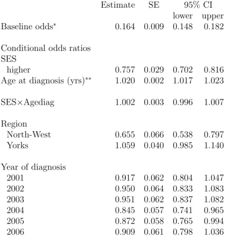
Estimate SE 95% CI lower upper Baseline odds⇤ _{0.164 0.009 0.148} _0.182

higher 0.757 0.029 0.702 0.816 Age at diagnosis (yrs)⇤⇤ _{1.020 0.002 1.017} _1.023

SES_⇥Agediag 1.002 0.003 0.996 1.007 Region North-West 0.655 0.066 0.538 0.797 Yorks 1.059 0.040 0.985 1.140 Year of diagnosis 2001 0.917 0.062 0.804 1.047 2002 0.950 0.064 0.833 1.083 2003 0.951 0.062 0.837 1.082 2004 0.845 0.057 0.741 0.965 2005 0.872 0.058 0.765 0.994 2006 0.909 0.061 0.798 1.036

Table 3: Results of logistic regression of Stage at diagnosis (one component ofM1) on SES

(A), Age at diagnosis (the other component ofM1), and Region and Year of diagnosis (C)

including the interaction between SES and age at diagnosis. Stage at diagnosis is coded 1 for advanced and 0 for early.

⇤ _{estimated odds of being diagnosed at an advanced stage for women diagnosed in the}

North East region in 2000, with low SES and aged 62 years at diagnosis.

(32)

Estimate SE 95% CI lower upper Baseline mean (intercept)⇤ 61.36 0.247 60.88 61.85 Mean di↵erences / slopes

SES higher –1.53 0.168 –1.86 –1.20 Region North-West –0.488 0.383 –1.24 0.262 Yorks 0.442 0.170 0.109 0.775 Year of diagnosis 2001 0.616 0.309 0.011 1.22 2002 0.620 0.309 0.014 1.22 2003 1.36 0.303 0.765 1.95 2004 0.737 0.303 0.142 1.33 2005 1.13 0.302 0.542 1.73 2006 0.958 0.305 0.360 1.56 Residual standard deviation

13.87

Table 4: Results of linear regression of Age at diagnosis (one component ofM1, in years)

on SES (A) and Region and Year of diagnosis (C).

⇤ _{estimated mean age at diagnosis for women diagnosed in the North East region in 2000,} with low SES.

(33)

A M1 M2 M3 Y U