Regulation expression pathway analysis (REPA): a novel method to facilitate biological interpretation of high throughput expression profiling data

(1)

Regulation Expression Pathway Analysis (REPA):

A novel method to facilitate biological interpretation

of high throughput expression profiling data

Master of Science

Department of Computer Science

Memorial University of Newfoundland

Pranjal Patra

(2)

Abstract

In the past decade there have been great advances and emergence of new techniques in the field of gene expression profiling. As the popularity of these techniques grew, the amount of data that gets generated has also grown. The task of analyzing this data to create a global picture to identify the biological pathways that are relevant to the study has been addressed by many. These approaches (collectively termed as enrichment analysis) have also grown in sophistication and accuracy making them the default step following a gene profiling experiment. However, enrichment analysis approaches do not provide pointers to likely regulators in their results.

In this project we built a system called Regulation Expression Pathway Analysis or REPA to facilitate the biological interpretation of results from high throughput gene expression profiling experiments. In particular, we provide researchers with gene sets that were most active in the biological phenomenon under study and their likely regulators. Users can input the gene expression profile data from their expression profiling experiments in REPA and get a list of disturbed gene sets and inferred transcription factors that possibly regulate these gene sets.

To build this system first we processed the transcription factor binding data from the ENCODE project to quantify the strength of regulation that each transcription factor has on each gene set. Then we build a gene expression enrichment analysis system that can analyze the gene expression profiling data and list the most active

(3)

gene sets. Finally we combine the results from the previous two steps to arrive at a more complete picture that gives users information about not only the most active gene sets, but also about the most likely regulators of these gene sets.

(4)

Acknowledgements

I wish to thank several people for their advice and support throughout this disserta-tion process. Special gratitude is owing to Dr. Lourdes Pe˜na-Castillo, my supervisor, whose direction, consideration and encouragement were exemplary and greatly appre-ciated.

Guidance from many professors especially Dr. Oscar Meruvia-Pastor and support from my colleagues and friends was helpful in completing this thesis.

I also wish to dedicate this work to Maa and Baba for all their love and sacrifices for me and Rippy.

(5)

List of Figures

2.1 Flow of information in biological systems (Horspool 2008) . . . 13

2.2 Location of DNA in a cell (Mariana Ruiz 2012) . . . 13

2.3 The structure of the DNA double helix (Zephyris 2011) . . . 14

2.4 Comparison of a single-stranded RNA and a double-stranded DNA (Sponk 2011) . . . 15

2.5 Myoglobin protein 3D structure (AzaToth 2008) . . . 16

2.6 Steps in gene expression (Forluvoft 2007) . . . 17

2.7 Transcription factors working as activators (Kelvinsong 2012) . . . . 20

4.1 Transcription factor - Gene set association distribution . . . 57

4.2 Predictions per transcription factor . . . 59

4.3 Predictions per gene set . . . 61

4.4 Venn diagram indicating the number of TFs in common between MSigDB C3-TFT collection, ENCODE’s TFBD and REPA’s predictions. . . . 68

4.5 REPA vs GAGE plot for BMP6 dataset . . . 76

4.6 BMP6 dataset Venn diagram . . . 77

4.7 REPA vs GAGE plot for breast cancer dataset . . . 78

4.8 Breast cancer dataset Venn diagram . . . 78

(9)

LIST OF FIGURES

4.10 Infection of Influenza A viruses dataset Venn diagram . . . 79 4.11 Breast cancer case study results . . . 83 4.12 Infection of influenza A viruses case study results . . . 85

(10)

Chapter 1 Introduction

It is now common knowledge that the entire genetic information of an organism is coded in its DNA. Therefore the knowledge of the exact sequence of the DNA of an organism is a valuable resource in the quest to understand how that organism func-tions. In recent times great advances were made in the development of techniques that enable high speed DNA sequencing. Any method or technology that can deter-mine the exact order of the four bases of DNA is called a DNA sequencing technique. Another method that have grown in popularity is the expression profiling techniques which allow researchers to check the activity levels of thousands of genes at once. These gene expression profiling techniques are extremely useful in determining the functions of genes. The data generated from such methods is huge, but without proper interpretation, is not of much use.

Our project is in the field of bioinformatics, which is an interdisciplinary field dealing with the development and use of computer software and databases to facilitate and enhance biological research. The main objective of this project is to facilitate the biological interpretation of the results from gene expression profiling experiments. In particular, we provide researchers with gene sets (or biological pathways) associated

(11)

to the biological phenomenon under study and their likely regulators. Gene sets are set of genes which have some feature in common such as genes that are involved in a pathway. To achieve this goal we built a software system called Regulation Expression Pathway Analysis (REPA) where users can input the gene expression profile data from their expression profiling experiments and get a list of disturbed gene sets and inferred transcription factors that possibly regulate these gene sets.

REPA uses an enrichment analysis approach called Functional Class Scoring or FCS. Enrichment analysis are a set of software tools and techniques which attempt to interpret the data from gene expression profiling experiments by finding functions and pathways that summarize the observations. Over the past decade as expression profiling grew in popularity, the need for accurate enrichment analysis also grew. Many algorithms and software tools were developed to address this. An in depth review can be found in the paper (Khatri, Sirota, and Butte 2012).

In REPA, we have mainly two modules. The first module links the transcription factors to individual gene sets. The second module performs enrichment analysis on the gene expression data. Combining the results from these two modules allows REPA to predict three things:

• Transcription factors that may regulate a given pathway. This is the result from the first module.

• Pathways that are affected in the given experiment. This is the result from the second module.

• Transcription factors that are most likely regulating the pathways that are most affected in the study. This is the result of combining the output of the two modules.

(12)

Over a hundred systems were developed in the past decade for performing en-richment analysis in gene expression data. Some of the most widely used tools are Gene Set Enrichment Analysis or GSEA (Subramanian et al. 2005), and Parametric Analysis of Gene set Enrichment or PAGE (Kim and Volsky 2005). In 2009 a new method called GAGE, or Generally Applicable Gene-set Enrichmen (Luo et al. 2009), was published which could handle datasets of different sample sizes or experimen-tal designs. GAGE showed significantly improved results compared to GSEA and PAGE (Luo et al. 2009). For validation, we compared the second module of REPA to GAGE. The novel aspect of REPA is that we are using hypothesis based statistical testing to find regulators that control entire gene sets. Then we combine the results from the enrichment analysis module to present more detailed analysis of the data obtained from gene profiling experiments. Previous tools only perform enrichment analysis on the gene expression data and provide gene sets that are perturbed in the experiment whereas REPA also provides information about the likely regulators of the perturbed pathways.

This thesis is organized in 5 chapters. After this initial introductory chapter, we discuss the necessary biology that is required to understand this project in chapter 2. We also look at the work that has been done so far in this area, describe the problem statement, and existing solutions. In chapter 3 we take a detailed look at REPA and all its components. System validation and comparison is presented in chapter 4 followed by a conclusion in chapter 5. The work described in this thesis has been accepted for publication in the IEEE/ACM Transactions on Computational Biology and Bioinformatics journal and presented at the Great Lakes Bioinformatics Conference 2015.

(13)

Chapter 2 Background Knowledge and

Related Work

This chapter describes the biological concepts required to understand the work done.

2.1 Flow of information in biological systems

The process of transmission of the genetic information from the genome of an organism to its phenotype (i.e. the expression of observable characteristics as an individual) is a complex process. A simplified description is provided here, as it is necessary to the understanding of this project.

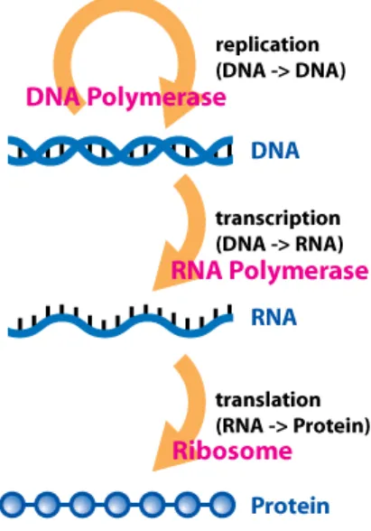
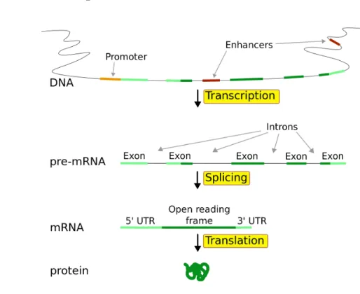
Figure 2.1 shows how genetic information flows within a biological system. This was first proposed by Frank Crick in 1958 and published later in 1970 (Crick et al. 1970). Generally this information flows from DNA to DNA (replication), DNA to RNA (transcription) and RNA to proteins (translation).

To fully understand the diagram we need to learn more about the macromolecules such as DNA, RNA, and proteins, along with processes such as replication, translation,

(14)

2.1. FLOW OF INFORMATION IN BIOLOGICAL SYSTEMS

Figure 2.1: Flow of information in biological systems (Horspool 2008) and transcription. This section describes each of them one by one.

2.1.1 Deoxyribonucleic acid (DNA)

The substance that is responsible for carrying the genetic information from parents to offspring in most living organisms, including all prokaryotic and eukaryotic cells and in many viruses, is an organic chemical of a complex molecular structure called Deoxyribonucleic acid, or DNA (Klug et al. 2012).

(15)

As shown in figure 2.2, DNA resides in the nucleus of eukaryotic cells, where inside the chromosomes, the DNA is condensed in a DNA - protein complex called chromatin. When the chromatin is uncoiled, its main component is revealed: the DNA molecule.

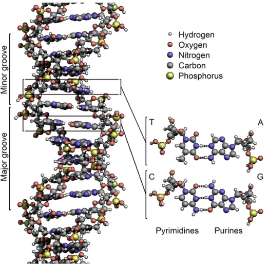
Figure 2.3: The structure of the DNA double helix (Zephyris 2011)

DNA has a double helix structure (Watson, Crick, et al. 1953), that looks like a long spiraling ladder (figure 2.3). It is formed of millions of elemental molecules, called nitrogenous bases, linked together in chains. The sequence in which the nitrogenous bases are linked amounts to a code that determines the characteristics of an individual, such as their eye color. These coded instructions are called genes. Genetic information is different for every individual making each of us unique.

(16)

The genetic material, or the DNA, of an organism contains instructions to control all everyday cellular activities (Hunter 2012). Bases, or nucleotides, are the building blocks of DNA, and there are four types: Adenine, Guanine, Cytosine and Thymine. The structure of these bases are given in the figure 2.3.

The configuration of the DNA molecule is highly stable, allowing it to act as a template for the replication of new DNA molecules, as well as for the production (transcription) of the related RNA (ribonucleic acid) molecule.

2.1.2 Ribonucleic acid (RNA)

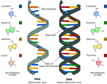
RNA is also a nucleic acid like DNA but unlike DNA it is a single stranded molecule. Another difference between the two is that instead of thymine the fourth base pair in RNA is uracil. The structural differences between the two nucleic acids are shown in figure 2.4.

Figure 2.4: Comparison of a single-stranded RNA and a double-stranded DNA (Sponk 2011)

(17)

There are different types of RNA molecules, but in this thesis we are only interested in the RNA molecule whose main function is to carry the genetic information from the DNA to proteins via the steps of transcription and translation. This type of RNA molecule is called messenger RNA or mRNA (Hunter 2012).

mRNA carries the coding instructions for protein synthesis from DNA to the ribosome. During translation, the mRNA molecule specifies the sequence of the amino acids in a polypeptide chain and thereby provides a template for joining amino acids. (Pierce 2005). The folding of these amino acid chains gives birth to a protein molecule.

2.1.3 Proteins

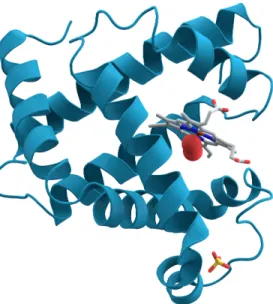
Figure 2.5: Myoglobin protein 3D structure (AzaToth 2008)

Proteins are large macromolecules that perform a wide array of functions. Each organism uses thousands of different proteins in their life span (Hunter 2012). Some functions that proteins perform are the catalyzation of metabolic reactions, the repli-cation of DNA, responses to stimuli, and the transportation of molecules from one

(18)

location to another, among many more.

For example, the protein myoglobin is an iron and oxygen binding protein. It is commonly found in the muscle tissues of vertebrates. It’s 3D structure is shown in figure 2.5 (Kendrew et al. 1958).

2.1.4 Gene

A gene is a unit of heredity in a living organism. A gene is usually responsible for influencing certain characteristics of the organism. It is normally a stretch of DNA that codes for a type of protein, or for an RNA molecule that has a function. Genes only have an effect on the cell when they are expressed (transcribed).

2.1.5 Gene expression

Figure 2.6: Steps in gene expression (Forluvoft 2007)

(19)

gene expression allows the information from a gene to be used in the synthesis of a functional gene product such as a protein molecule. Gene expression is of high impor-tance because by controlling which genes are expressed and which are not expressed in a given scenario, a cell can decide its phenotype and which proteins to synthesis. The process of gene expression involves several steps as shown in figure 2.6.

A section of the DNA is first transcribed and then translated. This section is called the transcription unit. Just above the transcription unit there is a sequence of nucleotides which defines where the transcription unit begins. This is known as the promoter region.

2.1.6 Transcription

Transcription is the process by which the information contained in a section of DNA (a gene) is transferred to a newly assembled piece of RNA. It is facilitated by RNA polymerase and transcription factors (described in section 2.2). In eukaryotic cells protein encoding transcripts (pre-mRNA) must be processed further in order to ensure translation.

2.1.7 Translation

In translation, messenger RNA (mRNA) produced by transcription is decoded by ribosomes to produce a specific amino acid chain, or polypeptide, that will later fold into an active protein molecule.

2.1.8 Putting it all together

So far in this section we have seen that, the genetic information that is passed on from parents to offspring in most living organism is stored in DNA. Genes are a

(20)

2.2. TRANSCRIPTION FACTORS

unit of heredity, and the entire genome of an organism could contain thousands of genes. An individual gene is usually a small stretch of DNA, that when expressed, codes for a specific protein. The process of gene expression involves several steps, namely transcription, splicing, and translation. The final product of gene expression is commonly a functional protein molecule. This way, the information that was passed on from the organism’s parents gets expressed and performs real functions in the organism.

2.1.9 Selective gene expression

Not every gene is expressed in all cells at all times. By controlling which genes are active, a cell can take on special characteristics and respond to its environment. Muscle cells and neurons have the same DNA, but perform different functions because they express different sets of genes. Transcription factors are one of the mechanisms to regulate which genes are expressed. In the nucleus, the DNA is condensed in the chromatin. In places close to where genes are being expressed, there are often zones of naked DNA. Transcription factors bind to these naked DNA sequences and regulate gene expression (Lyons 2012).

2.2 Transcription Factors

As mentioned above, transcription factors play a part in the regulation of gene expres-sion. Transcription factors are protein molecules that bind to a specific DNA sequence. Once bound to the matching DNA sequence, the transcription factor molecule can promote or block the transcription of a nearby gene. The location where the tran-scription factor attaches itself to the DNA is called the trantran-scription factor binding site. After binding itself the transcription factor regulates a gene that is spatially

(21)

2.2. TRANSCRIPTION FACTORS

near the binding location, for example, by making it easier for the RNA polymerase to attach to the gene’s promoter region. In most cases the gene lies downstream to the transcription factor binding site but in some cases, due to the complex nature of the three dimensional structure of the chromatin, a transcription factor can regulate a gene that is thousands of base pairs away but is close to the binding site in three dimensional space.

By promoting (as an activator), or blocking (as a repressor), the recruitment of RNA polymerase during transcription, transcription factors regulate the level of gene expression. RNA polymerase is the enzyme that performs the transcription of genetic information from DNA to RNA. Some transcription factors perform this function with other proteins in a protein complex while some do it alone.

Figure 2.7: Transcription factors working as activators (Kelvinsong 2012)

A demonstration of how these proteins affect the level of gene expression is given in figure 2.7. In this figure, several transcription factors are working together to create a protein complex that makes it easier for RNA polymerase to attach to the promoter

(22)

2.3. BIOLOGICAL PATHWAYS

region and start transcribing the gene. The gene that is being regulated here is located in a distant part of the DNA but due to the three dimensional folding of DNA in the chromatin, it is spatially close to the transcription factor binding site.

By regulating the gene expression, transcription factors enable different cells to perform different functions. For example, different genes are turned on in liver cells than those in skin cells and different genes are turned on in cancer cells than in healthy cells. Through the action of transcription factors, the various cells of the body, which all have the same genome, can function differently.

Roughly 8% of genes in the human genome encode transcription factors (Broad 2014). They play important roles in development, the sending of signals within the cell, and the events in a cell that lead to division and duplication, known as the cell cycle. Several human diseases are linked to mutations in transcription factors, such as hearing loss, congenital heart disease, and cancer (Villard 2004; Peters et al. 2002; Schott et al. 1998).

2.3 Biological Pathways

A biological pathway is a series of actions among molecules in a cell that leads to a certain product or a change in that cell. A pathway can trigger the assembly of new molecules, such as a lipids or proteins. Pathways can also turn genes on and off, or spur a cell to move. Some of the most common biological pathways are involved in metabolism, the regulation of genes, and the transmission of signals.

2.4 ChIP-X Experiments

Several in vivo experimental technologies such as chip (Iyer et al. 2001), ChIP-seq (Johnson et al. 2007), ChIP-PET (Wei et al. 2006) and DamID (Peric-Hupkes

(23)

2.5. GENE EXPRESSION PROFILING

et al. 2010) provide details about possible binding sites for transcription factors at a genome-wide level. These four methods together are referred to as ChIP-X. The sites discovered using the ChIP-X methods are near genes and are found when the chromatin structure of a specific cellular state allows binding of a particular tran-scription factor. This means that unlike possible binding sites found using in vitro approaches, the possibility of these sites to have actual biological significance is much higher. Results from such experiments report the binding of specific transcription fac-tors to DNA in proximity of a target gene’s location. Such experiments commonly list hundreds to thousands of potential regulatory interactions (Lachmann et al. 2010).

2.5 Gene Expression Profiling

Gene expression profiling is the measurement of the abundance level (the expression) of thousands of transcripts at once, to create a global picture of cellular state. These profiles can, for example, distinguish between cells that are actively dividing, or show how the cells react to a particular treatment.

A DNA microarray (also commonly known as a DNA chip or biochip) is a collection of microscopic DNA spots attached to a solid surface. Scientists use DNA microar-rays to measure the expression levels of large numbers of genes simultaneously, or to genotype multiple regions of a genome. Each DNA spot contains segments of a specific DNA sequence, known as probes (or reporters or oligos). These can be a short section of a gene or other DNA element that are used to hybridize a cDNA or cRNA (also called anti-sense RNA) sample (called target) under high-stringency conditions. Probe-target hybridization is usually detected and quantified by detection of fluorophore-, silver-, or chemiluminescence- labelled targets to determine relative abundance of the targets in the sample. RNA-seq refers to the use of high-throughput

(24)

2.6. PATHWAY ANALYSIS OF GENE EXPRESSION DATA

sequencing technologies to sequence cDNA in order to get information about a sam-ple’s RNA content. The technique has been rapidly adopted in studies of diseases like cancer.

2.6 Pathway Analysis of Gene Expression Data

Gene expression profiling experiments allow biologists to measure the activity lev-els of genes. The data that is generated from such experiments usually is several megabytes long. For example in (Emery et al. 2009) and (Lavery et al. 2008), the research teams have performed typical gene expression profiling experiments and the data after refinement is 88 MB and 21.7 MB in size respectively. To derive useful information from this large quantity of data is a challenge. In the last decade or so, as experiments of such nature have gained popularity, several approaches have been devised to help researchers understand the meaning of this data and to determine the biological activities taking place in the cells under observation.

This thesis is in the research area of facilitating the researchers who are performing such experiments to understand the biological processes that are active in their studied cellular state. It is done by performing statistical tests on the data obtained from high throughput gene expression profiling experiments. Several individual research groups have made important contributions to this field and this project built upon the work that has been done so far. In the following sections, we discuss all those techniques and databases that are related to this project.

2.7 Gene sets formation

Individual genes are annotated based on their functions, position and other charac-teristics. For example, functional annotation for a gene can be its association with

(25)

2.8. ENRICHMENT ANALYSIS (PATHWAY ANALYSIS)

a particular function in a metabolic pathway. Any information about the function of this gene is a functional annotation of the gene. These annotations are stored in publicly available databases. Using these publicly available gene annotations it is possible to create gene sets by taking all the genes that have a common annotation and clubbing them together. Usually every biological pathway, such as metabolic or signaling pathways, are associated with certain genes. Thus, by clubbing together genes based on their functions, we can connect biological processes or pathways to sets of genes. An example of such a gene set could be the KEGG pathway Glycerolipid metabolism (hsa00561) (Kanehisa and Goto 2000). Based on published studies, there are 49 genes associated with the pathway (Norbeck et al. 1996; Karlsson et al. 1997; Berg et al. 2001). These genes form the glycerolipid metabolism gene set.

2.8 Enrichment Analysis (Pathway Analysis)

High-throughput gene expression profiling techniques, such as DNA microarray and RNA-Seq, allow researchers to simultaneously measure genome-wide levels of gene ex-pression under specific biological conditions. Statistical approches such as limma (Smyth 2005) and edgeR (Robinson, McCarthy, and Smyth 2010) are then used to identify differences in gene expression between two or more conditions. Enrichment analysis or pathway analysis is an analytical approach to interpret the results of a gene expression profiling experiments with respect to gene sets. It is the process with which we as-sociate observed changes in gene expression with cellular functions and/or metabolic pathways. Without such an analytical process, it will be very difficult to comprehend which biological pathways are most active in the particular case under study.

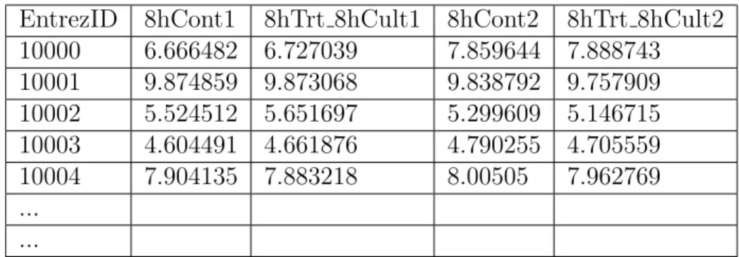
Gene expression profiling experiments usually generate a list of differentially expressed genes. Here is an example of how the data that is obtained from such an experiment

(26)

looks (Lavery et al. 2008).

EntrezID 8hCont1 8hTrt 8hCult1 8hCont2 8hTrt 8hCult2 10000 6.666482 6.727039 7.859644 7.888743 10001 9.874859 9.873068 9.838792 9.757909 10002 5.524512 5.651697 5.299609 5.146715 10003 4.604491 4.661876 4.790255 4.705559 10004 7.904135 7.883218 8.00505 7.962769 ... ...

Table 2.1: Expression profiling data sample

Such a list can be very useful in identifying genes that may have roles in a par-ticular phenomena or phenotype. However, for many researchers this list would not be sufficient in providing insight into the underlying biology of the condition being studied. To individually study each gene and interpret the meaning would be a very complex and time consuming process. Therefore, categorizing the genes based on their common functional annotation helps in two ways.

Reduced complexity By grouping the genes into sets of genes, with each gene

set targeting a specific pathway or function, the complexity is reduced to just a few hundred pathways for the experiment.

Higher explanatory power Pathways that have different activity levels between

two conditions would generally have a higher explanatory power than just a list of genes would (Glazko and Emmert-Streib 2009).

Hence the lower complexity and higher explanatory power of enrichment analysis has made it a de-facto in post gene expression analysis. Broadly, there are three different approaches for performing enrichment analysis (Khatri, Sirota, and Butte 2012). They are :

(27)

• Functional Class Scoring (FCS) approach.

• Pathway Topology (PT) approach.

We look at them one by one in the following sections.

2.8.1 Over-Representation Analysis (ORA) Approach

The growth in the popularity of High-throughput sequencing, and also the develop-ment of public gene set repositories such as Gene Ontology (GO) or Kyoto Encyclope-dia of Genes and Genomes (KEGG), fueled the immeEncyclope-diate need for functional analysis of microarray gene expression data. To tackle these problems the Over-Representation Analysis (ORA) approach was devised.

From the expression levels observed in the sequencing experiment, a list of signifi-cant genes that were over-expressed or under-expressed is created. To create this list, an arbitrary cut-off p-value is set. For example, a researcher may say that all genes that have a p-value less than, or equal to, 0.05 qualify as significant genes. Next, for each pathway (or gene set) the numbers of genes that are present in this list are counted. Then, by using statistical analysis techniques, such as tests based on the hyper geometric, chi-square, or binomial distribution, it is determined whether more genes belonging to the gene set are present in the list than expected by chance.

This is a very simple technique, but it sheds some light on the gene sets that are under or over expressed. ORA has a few shortcomings too, as discussed next.

Limitations of Over-Representation Analysis (ORA) Approach

Even though the ORA approach is the most popular approach, it has several short-comings.

(28)

Firstly, the statistical tests (e.g., hyper geometric distribution, binomial distribu-tion, chi-square distribudistribu-tion, etc.) ignore the measurements found for the genes in the gene expression experiments. As this data is ignored, all the genes that make the list are treated equally despite their varying levels of expression. The list of signifi-cant genes is generated based on an arbitrary threshold and the individual genes that do not make the threshold are discarded. Genes whose expression levels fall in the border of the threshold also have some significance but are totally ignored. This is a disadvantage of having a hard cutoff threshold.

Secondly, one of the goals of gene expression analysis is to understand how interac-tions between various gene products occur as the levels of gene expression changes. By considering that all the genes are independent, ORA significantly reduces its ability to analyze complex biological interactions that include several gene products. Because the ORA techniques consider all genes as equal and independent, it fails to provide any insight in this regard.

Finally, this approach works with the assumption that all the pathways are in-dependent to each other, which is not true. For example, in signaling pathways in KEGG, there is a presence of growth factors that activate the MAPK signaling path-way. This signaling pathway in turn activates the cell cycle pathpath-way. ORA methods do not account for such inter-pathway interactions and dependences.

2.8.2 Functional Class Scoring (FCS) Approach

In most biological systems, significant effects on pathways can be caused by large changes in individual genes, but they can also be caused by weaker coordinated changes in the expression levels of several functionally related genes. By clubbing such related genes into a gene set such that a gene set represents a biological path-way, we can detect such effects. Almost all the FCS based methods have mainly three

(29)

steps:

Step 1: Calculate Gene Level Statistic

First a gene level statistic is computed from the molecular measurement data obtained from high-throughput expression analysis experiments such as DNA microarray or RNA-Seq. This is done by calculating differential expression for each of the genes. Several statistical methods, such as correlation of molecular measurements with phenotype (Pavlidis et al. 2004), Q-statistic (Goeman et al. 2004), signal-to-noise ratio (Subramanian et al. 2005), t-statistic (Tian et al. 2005) or Z-score (Kim and Volsky 2005) can be used to represent the expression levels.

Step 2: Calculate pathway level statistics

Next, gene level statistics for all genes in a given gene set are aggregated into a single pathway level statistic. There are several statistical methods to do this but some of the more common ones are Kolmogorov - Smirnov (Smirnov 1944), the Wilcoxon rank sum test (Mann, Whitney, et al. 1947), or to take the sum, mean or median of the gene level statistics. Whatever method is chosen to implement this, it’s power can depend on factors such as the proportion of the genes present in the pathway that were differentially expressed, the actual size of the pathway (i.e. the number of genes present in the pathway) and the amount of correlation that exists between the various genes in the pathway. Even though multivariate statistics should show better results as they also account for inter-dependencies among genes, it has been observed that for higher cut-offs (pV alue≤0.001), the uni-variate statistics show more power, and for less stringent cut-offs (pV alue≤ 0.05) the uni-variate statistics show equal power (Khatri, Sirota, and Butte 2012).

(30)

Step 3: Assessing statistical significance of the pathway level statistic

In this step the statistical significance is computed by using a null hypothe-sis. There are mainly two ways to do the testing: competitive null hypothesis testing and self-contained null hypothesis testing. In the former method, class labels (i.e. phenotypes) for each sample are permuted, and comparison is made between the set of genes in a given pathway with itself. In the latter method, gene labels are permuted for each pathway, and comparisons are made between the set of genes that are in the pathway, with the set of genes that are not in the pathway. The size of the gene sets remains the same.

Advantage of using FCS

Some of the limitations described above related to using the ORA approach have been addressed in the FCS approach. This helps FCS provide better results and deeper insight into the underlying biology of any given condition than those provided by ORA. For example, FCS does not require any arbitrary cut-off threshold for dividing the genes into significant and non-significant groups. It uses all the available molecular measurements for its analysis. FCS uses the molecular measurement information to detect coordinated changes in expression of genes in some pathways. By detecting such coordinated changes, FCS can give us information about dependence between genes.

Limitations to FCS

FCS analyzes each pathway independently, hence a problem arises when a single gene is part of multiple pathways. In such a case, a given gene might be over-expressed because it is playing an important role in a particular pathway, but this expression level will be considered while evaluating the pathway level statistic of other pathways

(31)

that the gene is a part of. Another limitation arises when the statistical method used to implement FCS is a rank based method. In such a case, the value obtained in the experiment is not considered in the analysis, but only the rank assigned is considered.

2.8.3 Pathway Topology (PT)-Based Approach

Pathway topology is the newest technique available for performing enrichment analy-sis. It is similar to FCS, except for how pathway topology based-approaches compute the gene level statistics. Several publicly available pathway knowledge bases hold information about gene products that interact with each other, how those products interact and where they interact in a given pathway. ORA and FCS do not utilize this knowledge. An example of a PT-based approach is ScorePAGE proposed by (Rah-nenfuhrer et al. 2004). ScorePAGE computes similarity between each pair of genes in a pathway. The similarity is measured by calculating the correlation or covariance between the two genes. The similarity score is comparable to the gene level score in FCS based approaches. Then, these scores are averaged to arrive at the pathway level statistics. However, ScorePAGE divides the similarity score with the number of reactions needed to connect the two genes in the pathway. This strategy assigns varying weights to the pairwise similarity scores.

Limitations

Some of the common limitations with this strategy are:

• Pathway topology depends upon the cell type and the condition being studied. Hence this information is not readily available and is usually fragmented in various knowledge bases. As the annotation becomes more comprehensive and complete, these approaches are expected to perform better.

(32)

• No existing PT-based approach can collectively model and analyze high-throughput data as a single dynamic system.

(33)

Chapter 3 Methodology and Implementation

3.1 Motivation

In the modern day world a plethora of data is produced everyday in laboratories per-forming high throughput experiments such as DNA Sequencing and Gene Expression Profiling. Trying to analyze and understand the mechanisms of the biological pro-cesses under study is a non-trivial task. To extract knowledge from this data there is a need for new computer programs to perform analytics and help interpret this growing amount of data.

Some of the common questions that arise after any RNA sequencing or DNA microarray experiment are: what biological pathways were affected in the sample, and which transcription factors were regulating these biological pathways. Providing answers to these questions can help researchers to make new discoveries or provide direction to their future research.

Currently there are programs to identify the biological pathways that are getting affected. As discussed in Khatri et al (Khatri, Sirota, and Butte 2012) programs such as Gage (Luo et al. 2009) can identify the gene sets that are over or under expressed

(34)

3.2. OVERVIEW OF THE SYSTEM

in the sample by statistical testing. There are also programs such as ChEA (Kou et al. 2013) as described in the previous chapter that provide information about which transcription factors have their targets over-represented in a list of genes. Presently though, there is no such program that provides the full picture by predicting which transcription factor is actually regulating the pathways that are most affected in the study sample.

In this project, we combine the results of gene set enrichment analysis (FCS) and Chip-X data driven analysis to make predictions that tell the researcher which transcription factors might regulate pathways affected in the sample being studied.

3.2 Overview of the system

The software system that we built to materialize our idea had to perform several tasks. First, it should quantify to what degree a given transcription factor regulates any particular gene set. To achieve this, we performed a functional class scoring on the data obtained from the ENCODE project. Second, the software should identify which gene set was most affected in a given experiment. After conducting an exper-iment, researchers can use this software to perform functional class scoring on the data obtained from their experiment to reveal the biological pathways that were most affected. Finally, the system should combine the results of the above two parts to arrive at the final results. The final results will be a list of transcription factors and gene sets that are playing an important role in the phenomena under study.

(35)

3.3. REPA DESCRIPTION

3.3 REPA description

We will now look at the inputs to the system. Then, we will see each module in a greater detail. The modules of the system are as follows:

• Linking transcription factor binding sites with promoter regions of known human genes

• Creating the Regulation Database

• Expression Analysis

• Combining Regulation and Expression Results

3.3.1 Inputs to the system

There are mainly three inputs to the system.

Gene sets from gene annotation databases

As described in the previous chapter, a gene set is a group of genes that has some common functional annotation. A gene set may represent a biological pathway and include all the genes that play a role in that pathway.

For this project we gather our gene sets from two sources:

• Molecular Signatures Database or MSigDB

MSigDB (Subramanian et al. 2005; Liberzon et al. 2011) is a collection of anno-tated gene sets that were made publically available by various research groups such as Reactome (Vastrik et al. 2007), Biocarta (Nishimura 2001), Gene On-tology (Ashburner et al. 2000), Gene Arrays, KEGG (Kanehisa and Goto 2000; Kanehisa et al. 2014) and more.

(36)

MSigDB contains gene sets that are kept classified in six collections.

H Hallmark gene sets

Hallmark gene sets summarize and represent specific well-defined biological states or processes and display coherent expression. These gene sets were generated by a computational methodology based on identifying gene set overlaps and retaining genes that display coordinate expression (Total 50 gene sets).

C1 Positional gene sets

These are gene sets corresponding to each human chromosome and each cytogenetic band that has at least one gene. These gene sets are helpful in identifying effects related to chromosomal deletions or amplifications, dosage compensation, epigenetic silencing, and other regional effects (Total 326 gene sets).

C2 Curated gene sets

These are gene sets collected from various sources such as online pathway databases, publications in PubMed, and knowledge of domain experts. The gene sets in this group can be further classified into the following groups (Total 4725 gene sets).

CGP: chemical and genetic perturbations These gene sets represent

expression signatures of chemical and genetic perturbations. For each perturbation there is usually two sets: one set consisting of genes that show increase in expression levels (XXX U P) and another set consist-ing of genes that show lower expression levels denoted by (XXX DOW N) (Total 3395 gene sets).

(37)

These are usually compiled by domain experts and are canonical rep-resentation of any given biological process (Total 1330 gene sets).

CP:BIOCARTA: BioCarta gene sets These are genes derived from

BioCarta pathway database (Nishimura 2001) (Total 217 gene sets).

CP:KEGG: KEGG gene sets Genes derived from KEGG pathway database

(Kanehisa and Goto 2000; Kanehisa et al. 2014) (Total 186 gene sets).

CP:REACTOME: Reactome gene sets Genes derived from Reactome

pathway database (Vastrik et al. 2007) (Total 674 gene sets).

C3 Motif gene sets

Gene sets that contain genes that share a cis-regulatory motif that is con-served across the human, mouse, rat, and dog genomes (Xie et al. 2005) (Total 836 gene sets).

MIR: microRNA targets Gene sets that contain genes that share a

3’-UTR microRNA binding motif (Total 221 gene sets).

TFT: transcription factor targets Gene sets that contain genes that

share a transcription factor binding site defined in the TRANSFAC database (version 7.4) (Wingender 2008). Each of these gene sets is annotated by a TRANSFAC record (Total 615 gene sets).

C4 Computational gene sets

Computational gene sets defined by mining large collections of cancer-related microarray data (Total 858 gene sets).

C5 GO gene sets

These are the gene sets that are named after GO terms and contain genes annotated by that term (Total 1454 gene sets). The gene sets in this group can be further classified into the following groups.

(38)

BP: GO biological process Gene sets derived from the Biological

Pro-cess Ontology (Total 825 gene sets).

CC: GO cellular component Gene sets derived from the Cellular

Com-ponent Ontology (Total 233 gene sets).

MF: GO molecular function Gene sets derived from the Molecular

Func-tion Ontology (Total 396 gene sets).

C6 Oncogenic signatures

These gene sets represent signatures of cellular pathways which are of-ten dis-regulated in cancer. The majority of signatures were generated directly from microarray data from NCBI GEO (Edgar, Domrachev, and Lash 2002) or from internal unpublished profiling experiments which in-volved perturbation of known cancer genes. In addition, a small number of oncogenic signatures were curated from scientific publications (Total 1454 gene sets).

C7 Immunologic signatures

Gene sets that represent cell states and perturbations within the immune system (Total 1454 gene sets).

• KEGG: Kyoto Encyclopedia of Genes and Genomes

Kyoto Encyclopedia of Genes and Genomes (KEGG, http://www.genome.jp/ kegg/ or http://www.kegg.jp/) is a database that provides manually curated gene sets (Kanehisa and Goto 2000; Kanehisa et al. 2014). KEGG collects infor-mation on functional annotations of various DNA elements and integrates this information. Genes from completely sequenced genomes are linked to higher-level systemic functions of the cell, the organism and the ecosystem. Then this information is used to create a knowledge base for organizing experimental

(39)

knowledge in computable forms; namely, in the forms of KEGG pathway maps. Any KEGG pathway includes a list of all the genes which play a functional role in the pathway and also other details such as the pathway map and any diseases linked with this pathway. The genes in a given pathway form a gene set. In REPA we used the gene sets from KEGG along with the gene sets from MSigDB. We included directly KEGG pathways as gene sets, as we noted that MSigDB does not include the most recent version of the KEGG.

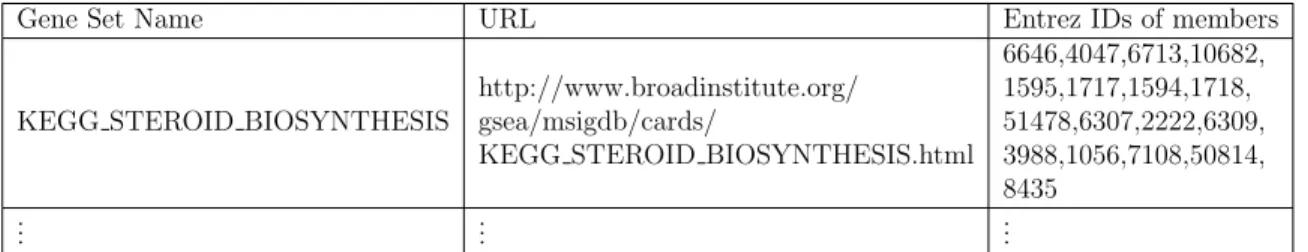
We represent gene sets in the format that is used by MSigDB. Namely first column gives the name of the gene set. The second column is not used by the program but specifies a URL that gives more information about the specific gene set. After that we have a list of entrez ids that specify the genes that are present in the gene set. The file is a tab delimited text file without headers. For example, table 3.1 shows the format of a sample gene set.

Gene Set Name URL Entrez IDs of members

KEGG STEROID BIOSYNTHESIS

http://www.broadinstitute.org/ gsea/msigdb/cards/

KEGG STEROID BIOSYNTHESIS.html

6646,4047,6713,10682, 1595,1717,1594,1718, 51478,6307,2222,6309, 3988,1056,7108,50814, 8435 .. . ... ...

Table 3.1: Sample Gene Set

Transcription Factor Binding Data (TFBD)

As described in the previous chapter in section 3.4.1 one of the goals of the public research project Encyclopedia of DNA Elements or ENCODE (Consortium et al. 2012) was to identify the transcription factor binding sites. The data produced under this project from numerous Chip-Seq (Johnson et al. 2007) and Chip-Chip (Iyer et al. 2001) experiments provide information about the binding sites of 160 transcription

(40)

factors in 44 cell lines. This data was then processed and used by ChEA2 (Kou et al. 2013). ChEA2 also made the processed data freely available for download on their website (Kou 2014).

The ENCODE data compiled by ChEA2 includes 920 experiments done in 44 cell-lines profiling 160 transcription factors for a total of approximately 1.4 million transcription-factor / target-gene interactions (Kou et al. 2013). This data is given in the bed format which includes the transcription factor, cell line, start and end of peaks, score and signal. The score and signal values are directly proportional to the strength of the binding between DNA and the given transcription factor at any given site. The score value is derived from the signal and lies between 0 and 1000 and it is proportional to the maximum signal strength. We use the signal strength as input to our algorithm.

Genomic positions of human genes

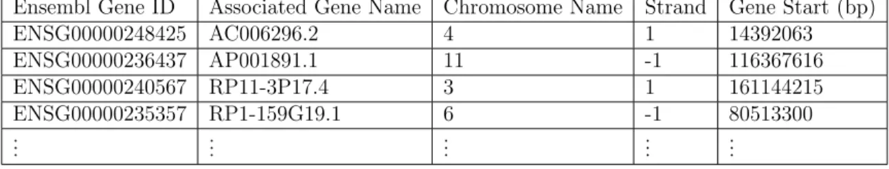
To link the transcription factor binding sites to the genes that the transcription fac-tors likely regulate, we needed the locations of both the transcription factor binding sites and the genes. As mentioned above, we got the ENCODE transcription factor binding sites data from ChEA2. For a list of all human genes and their position we used Ensembl’s Biomart (Kinsella et al. 2011) website http://www.ensembl.org/ biomart/martview/. Using this website we gathered the genomic positions of all human genes. The version that was used wasEnsembl Release version 71and the data set wasHomo sapiens genes (GRCh37.p10) (may 21, 2013). We included all genes coding for lincRNA, miRNA and proteins.

A sample of the data downloaded from Ensembl’s biomart website is given in table 3.2.

(41)

Ensembl Gene ID Associated Gene Name Chromosome Name Strand Gene Start (bp) ENSG00000248425 AC006296.2 4 1 14392063 ENSG00000236437 AP001891.1 11 -1 116367616 ENSG00000240567 RP11-3P17.4 3 1 161144215 ENSG00000235357 RP1-159G19.1 6 -1 80513300 .. . ... ... ... ...

Table 3.2: Ensembl Biomart Human Gene List

Gene expression profiling experiment data

After processing the results obtained from a high throughput gene expression profil-ing experiments such as DNA micro-array or RNA-seq a list with all the genes in the experiment with their corresponding level of activity is generated. To represent the gene level activity various types of statistics can be used. Some of the popular statis-tics user are log fold change, Z-statistic, t-statistic, etc. Table 3.3 gives an example of how the data looks.

Entrez ID logFC AveExpr t-statistic P.Value adj.P.Val 5228 4.066771195 8.984909943 30.01850012 1.75E-06 0.030867069 8200 -2.937752131 9.096127188 -22.30635557 6.85E-06 0.060528957 3400 3.107500295 8.990624466 18.99550122 1.43E-05 0.066519298 133 -3.11990311 9.026165624 -17.69540658 1.98E-05 0.066519298

Table 3.3: Sample gene expression profiling experiment data

3.3.2 Step 1: Linking transcription factor binding sites with

promoter regions of human genes

As discussed in (Kristiansson et al. 2009) “A gene’s promoter region is traditionally (if loosely) defined with respect to its transcription start site (TSS): 1000-3000 base pairs upstream, and 100-300 basepairs downstream.” In our project we focus on cis-regulated regions which are within 3000 base pairs upstream of the genes as the majority of the binding sites are located there. We ignored the enhancer regions which

(42)

are binding sites but typically at a much larger distance from the TSS.

We found all such instances where in the ENCODE data, a transcription factor binding site existed within 3000 base pairs upstream of a gene’s TSS.

Inputs to this part were the bed file with the location of the DNA - transcription factor binding peaks and the bed file with the genomic coordinates from the gene’s transcription start site to 3000 base pairs upstream for all human genes as described in section 3.3.1. We used Bedtools (Quinlan and Hall 2010) to accomplish this. Intersect command in Bedtools was used to find those promoter regions where a binding event occured. The command used was as follows:

i n t e r s e c t B e d −a e n c o d e . bed −b g e n e L i s t . bed −wo

The −wo flag writes side by side the original A and B entries plus the number of base pairs of overlap between the two features.

3.3.3 Step 2: Creating the Gene Set - Transcription Factor

Binding Database

The goal of this step is to associate a transcription factor with given gene sets based on the binding strength of that transcription factor with the promoter region of the genes in each gene set. In other words we want to find out whether a transcription factor may regulate a given gene set. To achieve this we ran a functional class scoring with the transcription factor binding signals associated to human genes and the gene sets obtained from MSigDB and KEGG.

As described in the previous chapter, a functional class scoring approach has three steps. First is to calculate the gene level statistic. Next step is to find a gene set level statistic using the gene level statistic and finally using null hypothesis testing we find out the statistical significance of the gene sets.

(43)

A step by step description of the process follows.

Inputs

1. Gene sets in the format described in the section 3.3.1.

2. Transcription factor binding data from the output obtained in step 1 de-scribed in section 3.3.2.

Step 2.1: Parsing and loading input files The two input files are parsed and

loaded in memory. A hash table is used to store the data to quickly access the values based on transcription factor name and the gene’s Entrez Id.

Steps 2.2 through 2.6 are performed for each transcription factor - gene set pair.

Step 2.2: Map TFBSs to strongest signal Get the signal values from the

tran-scription factor binding sites database for each of the gene in the gene set. If multiple values exist from different cell lines, the maximum value is considered. If there are values for at least 5 genes in the gene set we proceed to the next step else we skip to the next gene set - transcription factor pair.

Steps 2.3 and 2.4 are executed 1000 times.

Step 2.3: Generate vector with random signal values To run the permutation

test, we first generate a gene set of randomly selected genes of the same size as that of the real gene set. We collect the signal values for this randomly chosen gene set from the transcription factor binding database as done in step 2.2 for the real gene sets.

Step 2.4: Statistical hypothesis testing We use the following three statistical

tests in our program with the real gene set values and the random gene set values as input.

(44)

Two-sample pooled test (ALGLIB project; Broad 2014)

This test checks hypotheses about the fact that the means of two random variables X and Y which are represented by samples xS and yS are equal. In our case xS represents the signals from real gene sets we found in step 2.2 andyS represents the randomly selected signal in the step 2.3. The test works correctly under the following conditions:

• Both random variables have a normal distribution • Dispersions are equal (or slightly different)

• Samples are independent.

During its work, the test calculates t-statistic:

t

=

xS−yS r P (_xi−_xS)2+P (_yi−_yS)2 Nx+_Ny−2 1 Nx+Ny1

NX and NY are the sizes of X and Y respectively.

Note 1 If X and Y have a normal distribution, the t-statistic will have

Student’s distribution withNX+NY−2 degrees of freedom. This allows the use of the Student’s distribution to define a significance level corresponding to the value of the t-statistic.

Note 2 If X or Y are not normal, t will have an unknown distribution

and, strictly speaking, the t-test is inapplicable. However, according to the central limit theorem, as the sample sizes increase, the distribution of t tends to be normal. Therefore, if sample sizes are big enough, we can use the t-test even if X or Y is not normal. But there is no way to find what

(45)

values forNX and NY are big enough. These values depend on howX and

Y deviate from the normal distribution.

After running this test we store the right-tailed p-value. The null hypoth-esis for the right-tailed test is that the mean of yS is less than or equal to the mean of xS.

Two-sample unpooled test (ALGLIB project) Similar to the two-sample

pooled test, this test checks hypotheses about the fact that the means of two random variables X and Y which are represented by samples xS and

yS are equal. The test works correctly under the following conditions: • Both random variables have a normal distribution

• Samples are independent.

Unlike the previous test, for this test, dispersion equality is not required. During its work, the test calculates the t-statistic:

t

=

xS−yS r V ar(_xS) NX + V ar(_yS) NY

If X and Y have a normal distribution, the t-statistic will have Student’s distribution with DF degrees of freedom:

DF

=

(NX−1)(NY−1) (N_Y−1)c2+(N_X−1)(1−c2)

c

=

V ar(_XS) NX V ar(_XS) NX + V ar(_XS) NY

(46)

This allows the use of the Student’s distribution to define the significance level corresponding to the value of the t-statistic. Note 2 from the two sampled pooled test section is also applicable to this test.

Mann-Whitney U test The Mann-Whitney U-test (Mann, Whitney, et al.

1947; McKnight and Najab 2010; Bochkanov and Bystritsky 1947) is a non-parametric method which is an alternative to the two-sample Student’s t-test. This test is used to compare medians of non-normal distributions

X and Y. The test works correctly under the following conditions:

• X and Y are continuous distributions (or discrete distributions well-approximating continuous distributions)

• X and Y have the same shape. The only possible difference is their position (i.e. the value of the median)

• The number of elements in each sample is not less than 5 • The samples are independent

• Scale of measurement should be ordinal, interval or ratio (i.e. test could not be applied to nominal variables)

Here is a simple step by step description of how the Mann-Whitney U test works:

• Both samples (having sizes N and M) are combined into one array which is sorted in ascending order keeping track of which sample the element had come from.

• After sorting, each element is replaced by its rank (its index in array, from 1 toN +M).

• Then the ranks of the first sample elements are summarized and the U-value is calculated using the following formula:

(47)

U

=

N

×

M

+

N(N₂+1)

−

P

x_i

Rank

(

x

i

)

The mean of U equals 0.5×N ×M. If U is close to this value, the medians of X and Y are close to each other. If we know distribution quantiles, we can get the significance level corresponding to the value of U.

• For a big enough N and M, U could be approximated by the normal distribution with a mean of 0.5×N ×M and a standard deviation of

σ

=

q

N×M(N+M+1) 12

The p-value is calculated from the mean and standard deviation.

All the three tests mentioned above namely two-sample pooled test, two-sample unpooled test and Mann-Whitney U-test returns three p-values:

p-value for two-tailed test The null hypothesis here is that the medians for

the two samples are equal.

p-value for left-tailed test The null hypothesis here is that the median ofyS

is greater than or equal to the median of xS.

p-value for right-tailed test The null hypothesis is that the median of yS is

less than or equal to the median of xS.

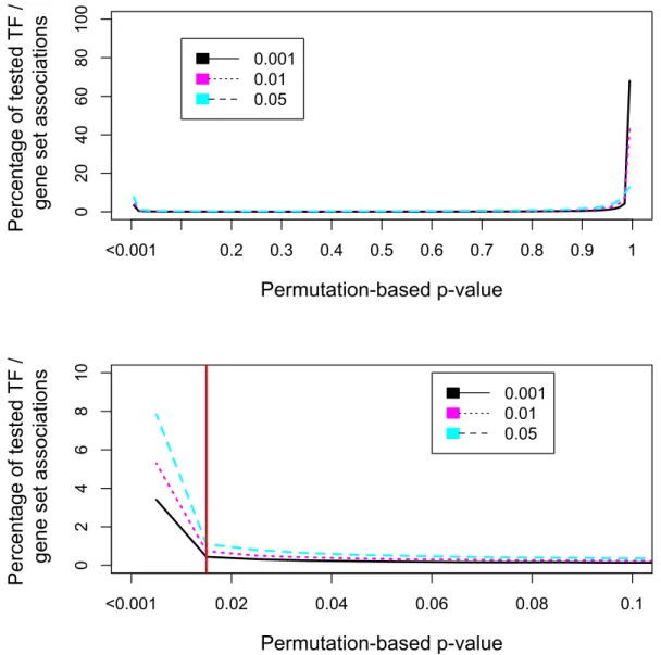
Step 2.5 For three pre-determined thresholds of significance namely 0.05, 0.01 and

0.001 we count number of times the mean / median of the values of the actual gene set is to the right of the mean / median of the values of the random gene set with a p-value of:

• less than 0.001

(48)

• between 0.05 and 0.01 • greater than 0.05

Transcription Factor E2F6

Gene set name DOANE BREAST CANCER CLASSES UP

Total genes in the gene set 72 Genes for which values were found 14 Pooled tTest [<0.001] 11 UnPooled tTest [<0.001] 7 MWU test [<0.001] 5 Pooled tTest [<0.01] 74 UnPooled tTest [<0.01] 75 MWU test [<0.01] 70 Pooled tTest [<0.05] 238 UnPooled tTest [<0.05] 237 MWU test [<0.05] 249 Pooled tTest [Remaining] 677 UnPooled tTest [Remaining] 681 MWU test [Remaining] 676 Pooled tTest Average p-value 0.1937 UnPooled tTest Average p-value 0.194217 MWU test Average p-value 0.18896 Genes in gene set for

which values were found 347, 253190, 51181 . . . . Table 3.4: Sample of the gene set - transcription factor binding database

Results After running the program for all the transcription factors and gene sets

available, the generated results are as shown in table 3.4. Due to space con-strains, the columns are presented as rows and rows as columns.

3.3.4 Step 3: Expression Analysis

The purpose of this step is to identify which gene set is over-expressed or under-expressed in the given biological sample. To achieve this goal, we used a functional class scoring approach.

(49)

1. Gene sets in the format described in the section 3.3.1

2. High throughput Gene expression profiling experiment data in the format de-scribed in section 3.3.1.

Step 3.1: Parse and load input data

First the two data files i.e. the expression levels and gene set database are read and loaded in the memory.

The following steps are executed for each available gene set in the database.

Step 3.2: Get expression levels for member genes of the gene set

For each of the genes present in the selected gene set, their corresponding values are retrieved and stored in a vector.

If the number of values found is greater than 5, proceed with the following steps.

Step 3.3: Create a random value vector of equal size

Here we select values from the expression levels files and insert them into a new vector. The number of values randomly selected and inserted are equal to the number of values found in the previous step.

Step 3.4: Running the statistical hypothesis tests

To understand the statistical significance of the values found in step 2, we com-pare them with the randomly generated values from step 3. We use the following three statistical hypothesis tests for this:

1. Two-sample pooled test 2. Two-sample unpooled test 3. Mann-Whitney U test

(50)

This step is similar to the step 4 in section 3.3.3 and the detailed description of the tests are also given in the same section.

Results After running the tests for all the available gene sets, we arrive at p-values

for each gene set for the particular case. We can conclude that the gene sets with the lowest p-values are either over-expressed or under-expressed. In either case their behavior is different from what is expected hence it can be concluded that there is a strong likelihood that the gene set is playing an important role in the cellular condition under study.

3.3.5 Step 4: Combining two p-values

From the two previous steps we have the following information:

From Step 2 A p-value quantifying the level of binding a transcription factor has

on a gene set.

From Step 3 A p-value representing the level of perturbation shown by any given

gene set in the experimental condition under study.

The next step is to combine the two p-values to obtain another p-value that rep-resents the likelihood of a transcription factor regulating the gene set in the biological condition under study.

To achieve this we follow the method suggested in the article titled ‘Combining p-values via averaging’ (Vovk 2012). In this article, the authors explains an old result by R¨uschendorf which shows that the p-values can be combined by scaling up their average by a factor of two. In our case since the there are only two p-values, we calculate the combined p-value as below:

(51)

3.4. BRIEF SURVEY OF EXISTING APPROACHES FOR ASSOCIATING TRANSCRIPTION FACTORS TO GENE LISTS

with K = 2

3.4 Brief survey of existing approaches for

associ-ating transcription factors to gene lists

The task of associating transcription factors with genes based on specific biological conditions has been tackled by some researchers. The work done in this field that we came across has been described and compared with in this section.

3.4.1 ChIP-X Enrichment Analysis (ChEA)

ChEA is a software tool that utilizes ChIP-X experiments data for linking tion factors to gene expression changes by computing over-representation of transcrip-tion factor targets in an input list of genes. ChEA essentially counts the number of targets in a list and compares them with the number of targets that were identified in the database, i.e. an ORA approach of transcription factor targets on an input list of genes (Lachmann et al. 2010).

ChEA is based on a manually curated database from the literature reporting ChIP-X experiment results. In this database, each record contains a list of genes potentially regulated by a specific transcription factor under a specific condition. This database was then used as the prior knowledge base to analyze mRNA expression data where enrichment analysis was performed. The current database as of September 2014 has the following statistics:

• Transcription Factors: 209

• Publications: 237

(52)

• Total Entries: 483786

ChEA is commonly used after a genome-wide gene expression profiling study is per-formed. The steps that follow are: First, a list of genes that significantly changed their expression levels is prepared and given as an input to the ChEA software. Next, the software computes over-representation for targets of transcription factors per study in the ChIP-X database. To compute statistical enrichment, ChEA implements the Fisher exact test with Bonferroni’s correction, where the proportions for the test are the number of genes in the input list, the number of genes identified in the ChIP-X experiment, the genes that are shared among the two lists, and the number of overall targets in the ChIP-X database. Finally, ChEA reports a ranked list of ChIP-X exper-iments that show statistically significant overlap with the input list. Identified genes from the input list, potentially regulated by a specific transcription factor, are also connected and visualized as a network, using known protein - protein interactions.

The ENCODE (Consortium et al. 2012; Raney et al. 2011) project was started with the main purpose of finding the functional elements of the human genome. Along with assigning function to DNA elements, a big part of the ENCODE project is to identify the transcription factor binding sites on the entire human genome.

The results from the experiments performed under ENCODE provide us with details about the location in the genome where a transcription factor binds and also the intensity of its binding. ChEA2 (Kou et al. 2013) also includes in its database all ChIP-X experiments from the ENCODE project.

Similarities between ChEA and REPA

The two programs are similar in the following ways:

• Both ChEA and REPA attempt to identify transcription factors regulating a col-lection of genes thereby predicting likely regulators of biological systems under

(53)

study.

• The data used by both ChEA2 and REPA comes from the ENCODE project.

Differences between ChEA and REPA

• REPA uses a functional class scoring algorithm instead of the over representation analyses approach used by ChEA. This allows REPA to identify gene sets instead of transcription factors that may regulate a list of genes that may or may not be co-functional. By using over representation analyses approach ChEA suffers from disadvantages arising from using hard cutoffs.

3.4.2 Inferring condition-specific transcription factor

func-tion from DNA binding and gene expression data

‘CRACR’ (McCord et al. 2007) (Combination Rank-order Analysis of Condition-specific Regulation; pronounced ‘cracker’), derives information about condition-Condition-specific gene regulation and transcription factor activity by combining comprehensive, condition-independent protein binding microarray (PBM) (Berger and Bulyk 2009) data for a given TF with gene expression microarray data under a variety of biological condi-tions. Specifically, CRACR searches for conditions in which differentially expressed genes are enriched or genes whose upstream intergenic regions (IGRs) contain a pat-tern to which a transcription factor has significant preference in PBM data. In contrast to earlier studies, CRACR integrates PBM-derived transcription factor sequence pref-erence data with gene expression data without imposing arbitrary cut-offs that define which IGRs are ‘bound’ or which genes are ‘differentially expressed’. In addition, CRACR uses rank order statistics, which facilitates comparison of gene expression data from different microarray platforms.

Regulation expression pathway analysis (REPA): a novel method to facilitate biological interpretation of high throughput expression profiling data