A simultaneous spatial autoregressive model for
compositional data
Thi Huong An Nguyen13, Christine Thomas-Agnan1, Thibault Laurent2& Anne Ruiz-Gazen1 1 Toulouse School of Economics, University of Toulouse Capitole, France
2 Toulouse School of Economics, CNRS, University of Toulouse Capitole, France 3 Danang University of Architecture, Vietnam
Abstract. In an election, the vote shares by party on a given subdivision of a territory form a vector with positive components adding up to 1 called a composition. Using a conventional multiple linear re-gression model to explain this vector by some factors is not adapted for at least two reasons: the existence of the constraint on the sum of the components and the assumption of statistical independence across territorial units questionable due to potential spatial autocorrelation. We develop a simultaneous spatial autoregressive model for compositional data which allows for both spatial correlation and correlations across equations. We propose an estimation method based on two-stage and three-stage least squares. We illustrate the method with simulations and with a data set from the 2015 French departmental election.
Keywords. multivariate spatial autocorrelation, spatial weight matrix, three-stage least squares, two-stage least squares, simplex, electoral data, CoDa.
1
Introduction
Some data present simultaneously the characteristics of compositional data (vectors with positive com-ponents conveying relative information) as well as the characteristics of spatial data (presence of spatial heterogeneity and spatial dependence). For example, land cover data contain information about different land use shares and the statistical unit is a subdivision of a territory; among the many papers that treat this type of data (see Leininger et al., 2013; Overmars et al., 2003; Yoshida and Tsutsumi, 2018; Pirza-manbein et al., 2018). Another instance is in geochemistry where data consist of composition of mineral deposits into chemical elements at different locations in geographical space, see for example Rubio et al. (2016) who study sediments in an artic lake or Filzmoser et al. (2010) who examine the Kola moss layer composition data from the R package StatDA (Filzmoser, 2020). This is also the case in political economy for electoral data containing the vote shares by party in a multiparty election for a list of administrative subdivisions of a territory as in Katz and King (1999) or for data about turnout rates as in Borghesi and Bouchaud (2010). Other examples include the distribution of temperature data at weather stations as in Salazar et al. (2015), the distribution of benthic macroinvertebrates at sampling stations in the Delaware Bay in Billheimer et al. (1997).
The challenge for modelling such data is to accomodate at the same time their compositional and spatial nature. For spatial data with a continuous domain, Pawlowsky and Burger (1992); Pawlowsky-Glahn and Egozcue (2016); Rubio et al. (2016); Martins et al. (2016) adopt a geostatistical approach. On the other hand, conditional autoregressive models have been developed for the multivariate regression framework (MCAR), e.g. Mardia (1988) and Gelfand and Vounatsou (2003). An application of MCAR to compositional data can be found in Billheimer et al. (1998) where vectors of counts are modelled by multinomial distributions whose parameters follow a prior Gaussian Markov random field. These hier-archical Bayesian models need Markov Chain Monte Carlo procedures for fitting. As in our application, Pirzamanbein et al. (2018) and Leininger et al. (2013) deal with areal data. Pirzamanbein et al. (2018) combine a Dirichlet distribution with a Gaussian Markov random field prior for the alr transformed vec-tor of Dirichlet parameters. Leininger et al. (2013) propose a power transformation combined with an MCAR model in order to address the problem of observed zero proportions. We choose to focus rather
on a combination of ilr transformations with a spatial econometrics model which has the advantage of a very easy implementation involving only ordinary least squares steps. The compositional vector being the dependent variable, we will need spatial econometrics models for multivariate dependent variable as in Kelejian and Prucha (2004). We develop a simultaneous spatial autoregressive model for compositional data (CoDa) which allows for both spatial correlation and correlations across equations. We propose an estimation method based on two-stage (S2SLS) and three-stage (S3SLS) least squares.
In Section 2, we first recall some classical facts adapted to work with CoDa. We then introduce a new operation which will be necessary later to write our model in a simplex fashion and study its properties. In Section 3, we recall facts about the definition and estimation of simultaneous autoregressive models for multivariate output spatial data and combine with the tools of Section 2 to define our model for spatio-compositional data. Section 4 presents some simulations to evaluate the quality of the S2SLS and S3SLS methods in the multivariate case. Section 5 presents an application to election results with the question of the impact of socio-economic variables on parties vote shares with a data set from the 2015 French departmental election. Section 6 concludes.
2
Definitions and notations in compositional data analysis
AD-compositionuis a vector ofD parts of some whole which carries relative information and therefore can be represented in the so-called simplex space SD defined by Aitchison (1986):
SD= ( u= (u1, . . . , uD)T :um>0, m= 1, ..., D; D X m=1 um= 1 ) ,
whereT is the transposition operator. For any vectorw∈
R+D,the closure operation is defined by
C(w) = w1 PD m=1wm ,· · · , wD PD m=1wm ! .
Let us recall the usual operations used to define a vector structure on the simplex space.
1. ⊕is the perturbation operation, corresponding to the addition inRD:
u⊕v=C(u1v1, . . . , uDvD), u,v∈SD
2. is the power operation, corresponding to the scalar multiplication inRD:
λu=C(uλ1, . . . , uλD), λ is a scalar,u∈SD
Moreover, the compositional product of a matrix by a vector denoted by is defined as follows
B u=C D Y m=1 ub1m m ,· · ·, D Y m=1 ubLm m !T
whereu∈SD,B= (blm) withl= 1, . . . L,m= 1, . . . , Dis aL×D matrix.
The simplexSDcan also be equipped with the compositional/Aitchison inner product (see Aitchison, 1985; Pawlowsky-Glahn et al., 2015) in order to define distances.
The analysis of compositional data makes use of log-ratio transformations which map the simplexSD to Rq (where most often q = D−1) because of their degree 0 homogeneneity (scale invariance). The
classical ones are the additive log-ratio (alr), the centered log-ratio (clr) and the isometric log-ratio (ilr) transformations. In this paper, we will mainly use some ilr transformations. Because it is needed to define the ilr, let us first recall the definition of the clr transformation of a vector u∈SD
clr(u) = ln um g(u) m=1,...,D , whereg(u) = D√u
1·u2· · ·uDis the geometric mean of the components. LetVDbe aD×(D−1) contrast matrix (e.g. Pawlowsky-Glahn et al., 2015) associated to a given orthonormal basis (e1,· · · ,eD−1) ofSD by
VD=clr(e1,· · ·,eD−1),
where clr is understood columnwise. For each such matrixVD, an isometric log-ratio transformation (ilr) is then defined by:
u∗= ilr(u) =VTDln(u)
where the logarithm ofu∈SDis understood componentwise. The inverse transformation is given by:
u= ilr−1(u∗) =C(exp(VDu∗)).
Since our data is made of samples of composition vectors, we store them in an×DmatrixY= (Yil),
i= 1, . . . , n, l= 1, . . . , D. Each row of this matrix, denoted byYi., is a compositional column vector of
SD. Y.l, l= 1, . . . , Ddenotes thelthcolumn of Yand we have
Y= [Y1.. . .Yn.]T = [Y.1. . .Y.D] (1) Let us define an extension of the ilr transformation of a matrixYby
ilr(Y) = ln(Y)VD= ilr(Y1.)T . . . ilr(Yn.)T
Note that ilr(Y) is an×(D−1) matrix.
In spatial econometrics models, spatial weight matrices are used to specify the neighborhood structure. Fornspatial locations, the elementswijof then×nmatrixWare measures of proximity between locations
i and j (see for instance Bivand et al., 2008, for different specifications). These matrices determine a covariance model for the data vector and play a role similar to the spatial variogram in geostatistics. For such a matrix and a given data vectorZof sizen, the lagged vectorWZcontains averages of the values of the variableZin neighboring locations whenWis row normalized. In our case, we need to apply such an operation to each column of the data matrixY and we wish that the application of this process to each column of Y results in a matrix in the same space as the original one (SD)n. As usual in CoDa, we use the principle of working in log-ratio coordinates (Mateu-Figueras et al., 2011) and expressing the results in the simplex. We thus define the following operation.
Definition 1. LetWbe an×nmatrix. The operation4· is a map from the cartesian product of simplex spaces (SD)n to itself defined by
W4·Y= ilr−1(Wilr(Y)) = ilr−1(Wln(Y)VD) (2)
Note that (W4·Y)∈(SD)n andWilr(Y)∈(R(D−1))n. This operation satisfies the following properties:
Proposition 1. Let Y be a n×D matrix such that each row, denoted by Yi., i = 1, . . . , n is a compositional vector in SD. LetW= (W
ij), (i, j= 1, . . . , n), an×nmatrix andα∈R. We have 1. W4·(αY) =α(W4·Y).
2. ilr(W4·(αY)) =αWilr(Y) =αilr(W4·Y).
3. (W4·Y)i.=CQn j=1Y Wij j1 ; Qn j=1Y Wij j2 ;. . .; Qn j=1Y Wij jD
, fori= 1, . . . , n, where (W4·Y)i.denotes theith row ofW4·Y.
4. LetY1,Y2∈(SD)n, thenW4·(Y1⊕Y2) = (W4·Y1)⊕(W4·Y2).
The proof of Proposition 1 is in the appendix. Note that property 3. implies that for each individual, each component of W4·Y is a weighted geometric mean of its neighboring values, weighted by the neighborhood weights.
3
Multivariate LAG regression model
The principle of compositional regression models is to use a transformation to send the data from the simplex to some coordinate space and to postulate a gaussian regression model in the coordinate space as in Egozcue et al. (2012). The model can then be transferred back to the simplex by the inverse transformation. In our case, the model in coordinate space must be a multivariate regression model because we have several response variables. For simplicity, we concentrate on the so-called LAG model which includes endogenous lagged variables on the right hand side of the model equations. An extension to a Durbin model would be immediate (LeSage and Pace, 2009). Since our model will be postulated in the coordinate space we choose to star all variables and parameters in Subsection 3.1. Note that the model we describe in Subsection 3.1 is not specific to CoDa.
3.1
Model in the log-ratio coordinates space
We consider a sample of size n and assume that we have M endogenous variables, hence M linear regression equations (M will be D−1 in Section 3.2). For a n×M matrix A, we will use the same notation as in Section 2 withA.l thelthcolumn, andAi.theithrow ofAas a column vector.
LetY∗ be an×M matrix of dependent variables andXbe an×K matrix of explanatory variables. We will allow for using a different set of explanatory variables in each equation. For this reason, we denote by SY∗
l , S X l , S
WY∗
l the sets of indices of the variables which appear in the l
th equation for Y∗, X, WY∗ respectively. AccordinglyY∗ SY∗ l ,XSX l ,Y ∗ SWY∗ l
will denote the columns ofY∗, X, WY∗
which appear in thelthequation.
Let ΓΓΓ∗= (Γ∗ml) andR∗= (R∗ml),(m, l= 1, . . . , M) beM ×M matrices of parameters. R∗ contains the parameters associated to the lagged endogenous variables on the right hand side of the model equation. As in the simultaneous equations literature in econometrics, each endogenous variable may also appear in each model equation so that ΓΓΓ∗ contains the corresponding parameters.
Finallyβββ∗is a K×M matrix of parameters for the explanatory variables.∗ denotes a n×M error matrix.
As in Kelejian and Prucha (2004), we consider the following model
Y∗.l= X m∈SY∗ l Γ∗mlY∗.m+XSX lβββ ∗ SX l + X m∈SWY∗ l Rml∗ WY.m∗ +∗.l (3)
Note that model (3) is written for each column of Y∗ i.e. for each component of the composition dependent vector but theM equations are linked by the covariance structure of the errors. Indeed, we assume that the errors are centeredE(∗) = 000M and thatE(∗i.∗j.) = ΣΣΣ∗ifi=jand 000 ifi6=j where ΣΣΣ∗is a (D−1)×(D−1) covariance matrix. This means that individuals are independent but that components of a given individual have a covariance structure ΣΣΣ∗.
Kelejian and Prucha (2004) suggest and study the properties of a Spatial Two Stage Least Square (S2SLS) procedure as well as a Spatial Three Stage Least Square (S3SLS) procedure to estimate model (3). Following their suggestion, we considerHa subset of linearly independent columns of then×3Kmatrix (X,WX, W2X). LetP
H =H(HTH)−1HT denote the projection matrix onto the space generated by the columns ofH. For the lth equation, we group the variables and parameters of the right hand side into a matrixZl of variables and a vectorδδδ∗l of parameters:
Zl= h YS∗Y∗ l XSX l WY ∗ SWY∗ l i ;δδδ∗l =hΓΓΓ.l∗T β∗lT R∗.lTi T .
The S2SLS estimation method for this model then proceeds as follows for each equation (i.e. each component) separately:
1. Perform a univariate regression of each column of ZonH and compute the fitted values ˜Zl: ˜ Zl=PHZl= h PHYS∗Y∗ l XSX l PHWY ∗ SWY∗ l i .
2. Perform a univariate regression ofY∗.l on ˜Zl: ˜
δδδ∗l = ( ˜ZTl Z˜l)−1Z˜Tl Y∗.l.
At the end of step 2, we can calculate the residuals by ˜
.l∗ =Y∗.l−Yˆ.l∗=Y.l∗−Zlδδδ˜
∗
l, and get an estimate of the covariance matrix ΣΣΣ∗ with
˜ Σ ΣΣ∗ml =˜ ∗T .m˜ ∗ .l n .
Until now, the covariance structure between equations has not been taken into account and the Three Stage Least Square (S3SLS) method is supposed to correct for this. To write the expression of the S3SLS estimator, we need to vectorize Y∗ (by stacking the columns of Y) resulting in y∗ = vec(Y∗) and to write the explanatory matrices as follows
Z= Z1 . . . 0 0 . .. 0 0 . . . ZM , ˜ Z= PHZ1 . . . 0 0 . .. 0 0 . . . PHZM .
We then get a corrected estimator ˆδδδ∗ ofδδδ∗
ˆ
δδδ∗= ( ˜ZT( ˜ΣΣΣ∗−1⊗In)Z)−1Z˜T( ˜ΣΣΣ∗−1⊗In)y∗ (4)
It is known that if the matrix R∗ is not diagonal, the S2SLS ˜δδδ∗ and S3SLS ˆδδδ∗ estimators are identical (see Greene, 2003, p. 488).
In the application of Section 5, we consider a slightly more general model in which we include com-positional variables among the explanatory (see for example Filzmoser et al., 2018). The additional complexity is the same as for a non-spatial model hence for the sake of simplicity we did not consider this extra layer in this section.
3.2
Writing the LAG regression model in the simplex space
Starting now with a sample of compositional vectors Y in SD, and given an ilr transformation, we postulate a model like (3) for the ilr coordinates ofY. Applying the ilr inverse transformation to each of the equations of model (3) withM =D−1 and using Proposition 1, we easily get that the system of equations (3) is equivalent to the system
Yi.=RT (W4·Y)i. K
M
k=1
Xikβββk⊕ΓΓΓT Yi.⊕i. (5)
whereRis aD×Dmatrix of parameters and where the model is now written at the individual level for all components simultaneously whereas in (3) it was at the component level for all individuals simultaneously. A more global way of writing the model for the whole matrixY would be the following
Y= (W4·Y) R⊕Xβββ⊕Y Γ⊕, (6)
where for an×D matrixUwhose rows are simplex valued and aD×D matrixB,the productU Bis an extension of the matrix product understood as then×Dmatrix whose rows are theBT U
i.vectors. One can write relationships between parameters in coordinate space and parameters in the simplex. The classical relationship betweenβββ andβββ∗ remains the same as in non spatial models (see for example Filzmoser et al., 2018)
βββk = ilr−1(βββk∗) =C(exp(VDβββ∗k)). Considering RT (W4·Y)i. and ΓΓΓT Y
i. as compositional explanatory, the relationships between R andR∗ and betweenΓandΓ∗ are as follows (see Chen et al., 2017)
R=VDR∗VTD and Γ=VDΓ∗VTD. (7)
Equations (7) also allow to establish the link between the parameters in coordinate space for two different ilr transformations. Coming back to the simplex after fitting the model allows to get rid of the possible arbitrary choice of ilr transformation. These relationships are true for population parameters and the next question is whether they still hold for the estimated parameters. Indeed the result holds because the two steps of S2SLS are based on ordinary least squares and we know that this method preserves the relationship for estimated parameters (see e.g. Nguyen, 2019).
4
Simulation
A simulation study of the performance of the S2SLS and S3SLS methods can be found in Das et al. (2003) but it is restricted to the case of a single dependent variable. For this reason, we now investigate by simulation the properties of the estimatorsβββ∗, R∗ and ΣΣΣ∗ of the S2SLS and S3SLS methods in the
multivariate spatial autoregressive model. We consider the n= 283 cantons of the Occitanie region in France with a neighborhood structure based on 10 nearest neighbors. All theRcode, graphs and tables are gathered in the supplementary material available online.1
For a number of replications N = 1 000, we simulate three explanatory variables X1,X2 and X3 following the Gaussian distributionsN(0,9),N(0,6) andN(0,9) respectively. When simulating the two dependent variables, we include all explanatory variablesX1,X2 andX3in each of the two equations.
1See
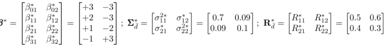
The parameterβββ∗, the covariance matrix ΣΣΣ∗and the matrixR∗are respectively assigned the following values β β β∗= β01∗ β02∗ β11∗ β12∗ β21∗ β22∗ β∗ 31 β32∗ = +3 −3 +2 −3 +1 −2 −1 +3 ; ΣΣΣ∗d¯= σ211∗ σ12∗ σ21∗ σ222∗ = 0.7 0.09 0.09 0.1 ; R∗d¯= R∗11 R∗12 R∗21 R∗22 = 0.5 0.6 0.4 0.3
Alternative diagonal matrices for ΣΣΣ∗ andR∗ are also considered
Σ Σ Σ∗d= 0.7 0 0 0.1 ; R∗d= 0.5 0 0 0.3 .
It is important to note that such a model is defined primarily in the simplex and has different repre-sentations in coordinate space according to the choice of ilr transformation. Therefore, constraining the matrixR∗ to be diagonal for a given ilr transformation does not imply that, for the same model in the simplex, the matrixR∗ would be diagonal with a different choice of ilr.
Note that the results are not too sensitive to the simulation framework except for the estimates of the error variances when the noise to signal ratio becomes too large. We consider four data generating processes (DGP) respectively denoted by ΣΣΣ∗d¯R∗d¯, ΣΣΣ∗d¯R∗d, ΣΣΣ∗dR
∗ ¯ d and ΣΣΣ ∗ dR ∗
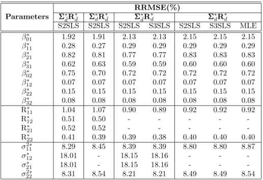
d according to the choice of matrices ΣΣΣ∗ andR∗.For each DGP, we calculate a Monte Carlo performance measure of the estimators proposed in Section 3 and for the MLE estimators in the diagonal case. The performance is measured by the relative root mean squared error (RRMSE), which is defined for an estimator ˆθ of a parameterθ by:
RRMSE(ˆθ) = RMSE(ˆθ) |θ| with RMSE(ˆθ) = v u u t 1 N N X i=1 ˆ θ(i)−θ2.
Table 1 presents the RRMSE for the S2SLS method, S3SLS and ML methods for all DGPs. We did not report the relative bias in Table 1 because its value is quite similar to the RRMSE showing that the bias dominates the error. The percentage of error is generally small with a maximum of 18.16% for the variance parameters and values less than 2.15% for the other parameters. For all DGPs, the largest differences between the estimates occur for the estimation of the intercepts and for the estimation of the R∗ matrix and these differences are small in all cases. We have done more simulations for other values of ΣΣΣ∗andR∗. The code is presented in the supplementary material and yields very similar results. Concerning theβββ andR estimates, only the S2SLS results are reported since S3SLS yields exactly the same results for the first two DGPs as proved by the theory. Concerning the variance estimates, note that there is no difference in its computation for the S2SLS and S3SLS. Finally, if we compare the three estimates in the case of DGP ΣΣΣ∗dR∗d, we can see that the results are quite close showing that S2SLS is a practical alternative to maximum likelihood in the framework of this model.
5
Application to political economics
Vote share data of the 2015 French departmental election of the Occitanie region in France are collected from the Cartelec website2. Corresponding socio-economic data (for 2014) are downloaded from the INSEE website3. The number of political parties presenting candidates at that election is higher than 15. However for simplicity reasons and due to the particular interest in the extreme right party in France,
2https://www.data.gouv.fr/fr/datasets/elections-departementales-2015-resultats-par-bureaux-de-vote/ 3https://www.insee.fr/fr/statistiques
Table 1: The RRMSE (in %) for all DGPs and parameters Parameters RRMSE(%) Σ ΣΣ∗d¯R∗d¯ ΣΣΣ ∗ dR ∗ ¯ d ΣΣΣ ∗ ¯ dR ∗ d ΣΣΣ ∗ dR ∗ d S2SLS S2SLS S2SLS S3SLS S2SLS S3SLS MLE β∗01 1.92 1.91 2.13 2.13 2.15 2.15 2.15 β∗11 0.28 0.27 0.29 0.29 0.29 0.29 0.29 β∗21 0.82 0.81 0.77 0.77 0.83 0.83 0.83 β∗31 0.62 0.63 0.59 0.59 0.60 0.60 0.60 β∗02 0.75 0.70 0.72 0.72 0.72 0.72 0.72 β∗12 0.07 0.07 0.07 0.07 0.07 0.07 0.07 β∗22 0.15 0.15 0.15 0.15 0.15 0.15 0.15 β∗32 0.08 0.08 0.08 0.08 0.08 0.08 0.08 R∗11 1.04 1.07 0.90 0.89 0.92 0.92 0.92 R∗12 0.51 0.50 - - - - -R∗21 0.52 0.52 - - - - -R∗22 0.41 0.39 0.39 0.38 0.40 0.40 0.40 σ112∗ 8.29 8.45 8.39 8.39 8.80 8.80 8.87 σ∗12 18.01 - 18.15 18.16 - - -σ∗ 21 18.01 - 18.15 18.16 - - -σ2∗ 22 8.31 8.54 8.21 8.21 8.49 8.49 8.54
we have aggregated them into three main components: Left, Right and Extreme-Right4. The dependent variable is thus a compositional variable which contains the vote shares of Left, Right and Extreme Right party. Cantons with at least one missing value on one of the components of the dependent vector have been eliminated resulting inn= 207 cantons in the final dataset. The loss of information is substantial and may cause bias. However the main focus of this paper is to illustrate the methodology. We use the following contrast matrix for D= 3 (see e.g. Pawlowsky-Glahn et al., 2015, p. 40)
V3= 2/√6 0 −1/√6 1/√2 −1/√6 −1/√2 .
This particular matrix defines the following ilr coordinates ilr1(x) = √1 6(2 logx1−lnx2−logx3) = 2 √ 6log x1 √ x2x3 ilr2(x) = √1 2(logx2−logx3) = 1 √ 2log x2 x3 .
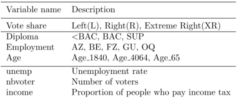
With this choice, the first ilr coordinate opposes the Left wing to the geometric mean of the Right wing and the Extreme Right party and the second opposes the Right wing to the Extreme Right party. Our explanatory variables, presented in Table 2, include both compositional and classical variables. For the three compositional variables, Diploma, Employment and Age, the log-ratio coordinates have been calculated using contrast matrices built from sequential binary partitions (see Nguyen, 2019, for details). The categories of these variables are as follows
• Employment has five levels: AZ (agriculture, fisheries), BE (manufacturing industry, mining indus-try and others), FZ (construction), GU (business, transport and services) and OQ (public admin-istration, teaching, human health),
Table 2: Data description. Variable name Description
Vote share Left(L), Right(R), Extreme Right(XR) Diploma <BAC, BAC, SUP
Employment AZ, BE, FZ, GU, OQ Age Age 1840, Age 4064, Age 65 unemp Unemployment rate
nbvoter Number of voters
income Proportion of people who pay income tax
• Diploma has three levels: <BAC for people with at most some secondary education, BAC for people with at least some secondary education and at most a high school diploma, and SUP for people with a university diploma,
• Age has three levels: Age 1840 for people from 18 to 40 years old, Age 4064 for people from 40 to 64 years old, and Age 65 for elderly.
An additional variable measuring the number of voters in each canton has been included to take into account a potential size effect.
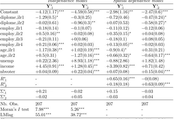
This data set has been analyzed in Nguyen and Laurent (2019) without taking into account the spatial structure and at a different spatial scale. We use model (3) in the coordinate space with ΓΓΓ∗= 0. Indeed, the reason for including spatially lagged dependent variable in the equations is for taking into account the spatial dependence and this justifies terms such as P
m∈SWY∗
l R
∗
mlWY∗.m in model (3). But in our case, there is no economic reason for introducing terms such asP
m∈SY∗ l
Γ∗mlY∗.m on the right hand side of the equations in the coordinate space. There is also no reason for assuming that the R∗ matrix is diagonal for this particular choice of ilr transformation and therefore, we do not impose this constraint. One important consequence of this choice is that, as we mentioned before, S2SLS yield the same results as S3SLS so that we carry out the S2SLS method from Section 3 for estimating the parameters.
First of all, for comparing the independence model to the spatial dependence one, we compute Moran test statistic of the residuals as well as the LMlag test statistics (separately for each ilr) and these indicate that the LAG model is preferable. Then looking at the size effect in Table 3, the number of voters is significant in both spatial and non-spatial model in the 2nd component (indeed there is some heterogeneity in the distribution of the number of voters at the canton level). The spatial dependence parameters (elements of the matrixR∗) are significant on the diagonal showing that a spatial dependence phenomenon is present in this data. The sign and significance of mostβββ parameters are very comparable, except in few cases (the unemployment rate, proportion of people who pay income tax, diploma and age variables) for which the significance changes from one ilr coordinate to the other. Further interpretations of the model parameters in the spatial model would go through the impacts computations as in LeSage and Pace (2009). But one would have to develop this tool in a multivariate framework and this is out of the scope of the present work. When we will be able to do so, this spatial LAG model will allow to evaluate spillover effects across cantons.
6
Conclusion
Motivated by an example in political economics, we develop a simultaneous spatial autoregressive model for compositional data combining the simultaneous systems of spatially interrelated cross sectional
equa-Table 3: Multivariate independent and spatial regression models with compositional and classical ex-planatory variables
Independence model Spatial dependence model
Y.1∗ Y∗.2 Y.1∗ Y∗.2 Constant −4.12(1.17)∗∗∗ −4.59(0.58)∗∗∗ −2.98(1.16)∗∗ −2.47(0.6)∗∗∗ diplome ilr1 −1.29(0.5)∗ −0.3(0.25) −0.72(0.46) −0.47(0.24)∗ diplome ilr2 −0.02(0.61) −0.96(0.3)∗∗ +0.07(0.53) −0.58(0.27)∗ employ ilr1 −0.18(0.14) −0.1(0.07) −0.11(0.12) −0.12(0.06) employ ilr2 +0.5(0.16)∗∗ −0.02(0.08) +0.35(0.15)∗ +0.04(0.08) employ ilr3 −0.21(0.11) +0(0.06) −0.18(0.1) +0.08(0.05) employ ilr4 +0.21(0.06)∗∗∗ +0.02(0.03) +0.13(0.05)∗∗ −0.02(0.03) age ilr1 −1.17(0.38)∗∗ +1.02(0.19)∗∗∗ −0.9(0.4)∗ +0.31(0.21) age ilr2 +0.5(0.31) −1.27(0.16)∗∗∗ +0.66(0.32)∗ −0.64(0.17)∗∗∗ unemp +0.22(2.36) +8.93(1.18)∗∗∗ −0.88(2.86) +1.82(1.48) income +4.45(0.91)∗∗∗ +1.28(0.45)∗∗ +3.39(0.82)∗∗∗ +0.71(0.42) nbvoter +0.04(0.09) +0.22(0.04)∗∗∗ +0.07(0.08) +0.15(0.04)∗∗∗ R∗.1 - - +0.65(0.16)∗∗∗ −0(0.08) R∗.2 - - +0.18(0.18) +0.63(0.09)∗∗∗ Σ∗.1 +0.21 −0.02 +0.15 −0.03 Σ∗.2 −0.02 +0.05 −0.03 +0.04 Nb. Obs. 207 207 207 207 Moran’sI test 7.98∗∗∗ 5.26∗∗∗ - -LMlag 55.01∗∗∗ 38.72∗∗∗ - -Note: ∗p<0.1;∗∗p<0.05;∗∗∗p<0.01
tions of Kelejian and Prucha (2004) and the compositional regression models (Filzmoser et al., 2018, e.g.). We propose an implementation using spatial two-stage and three-stage methods which are easy to implement.
There are several directions we could consider to go further in this framework. We could first of all consider alternative estimation methods. For example partial least squares procedures for the Spatial LAG model have been proposed in Wang et al. (2019) but for a single dependent variable. Similarly and with the same restriction, Spatial regression trees are developed for the LAG model in Wagner and Zeileis (2019). In a different direction, the aggregation of political parties in three blocks could be reconsidered. On the one hand, this aggregation avoids the zero problem due to the absence of some parties in some cantons but on the other hand it results in an information loss: imputation methods could be used to solve this as in Palarea-Albaladejo and Mart´ın-Fern´andez (2015). An extension to multivariate spatial error models (SEM) does not seem too complex but would need an additional step in the S3SLS procedure as in Kelejian and Prucha (2004). Finally, concerning the interpretation of the parameters of the spatial model, two possibilities have to be explored further. The first one is the interpretation in coordinate space. In a spatial model, interpretation of the parameters goes through the computation of impacts but to our knowledge, this has never been done in the multivariate LAG model. The second one is to obtain interpretations of the parameters in the simplex as in Morais et al. (2018) which implies being able to write the reduced form of the model in the simplex space.
7
Acknowledgements
We acknowledge funding from the French National Research Agency (ANR) under the Investments for the Future (Investissements d’Avenir) program, grant ANR-17-EURE-0010
8
Appendix
Proof of Proposition 1. LetY∈SD,Wbe an×nmatrix,αbe a scalar, and let (W4·Y)
i.denotes theithrow ofW4·Y,i, j= 1, . . . , n, l, m= 1, . . . , D.
1. ilr(W4·(αY)) = ilr(W4·Yα) =αWlnT(Y)V
D=αWilr(Y) =αilr(W4·Y). 2. We have
ilr(W4·(αY)) = ilr(W4·Yα) =αilr(W4·Y) then
ilr−1(ilr(W4·(αY))) = ilr−1(αilr(W4·Y)) =α(W4·Y) Thus,
W4·(αY) =α(W4·Y).
3. We have
(W4·Y)i.= ilr−1(ilr((W4·Y)i.)) = ilr−1(Wilr(Y))i. =C(exp(Wilr(Y)VTD)i.) where (Wilr(Y)VTD)i.= ln n Y j=1 Yj1 QD l=1Y 1/D jl !Wij ; ln n Y j=1 Yj2 QD l=1Y 1/D jl !Wij ;. . .; ln n Y j=1 YjD QD l=1Y 1/D jl !Wij . Thus, (W4·Y)i.=C n Y j=1 Yj1 QL l=1Y 1/D jl !Wij ; n Y j=1 Yj2 QL l=1Y 1/D jl !Wij ;. . .; n Y j=1 YjD QL l=1Y 1/D jl !Wij =C n Y j=1 YWij j1 ; n Y j=1 YWij j2 ;. . .; n Y j=1 YWij jD
4. LetY1,Y2∈(SD)n, and letY1∗= ilr(Y1),Y2∗= ilr(Y2), then ilr−1(ilr(W4·(Y1⊕Y2))) = ilr−1(W(Y∗1+Y
∗
2)) = ilr−1(WY∗1+WY∗2)
= ilr−1(Wilr(Y1) +Wilr(Y2)) = ilr−1(ilr(W4·Y1) + ilr(W4·Y2))) = ilr−1(ilr(W4·Y1))) + ilr−1(ilr(W4·Y2))) = (W4·Y1)⊕(W4·Y2)
Thus,
References
Aitchison, J. (1985). A general class of distributions on the simplex. Journal of the Royal Statistical Society. Series B (Methodological), 47(1):136–146.
Aitchison, J. (1986). The Statistical Analysis of Compositional Data. Chapman and Hall, London. Reprinted in 2003 with additional material by the Blackburn Press.
Billheimer, D., Cardoso, T., Freeman, E., Guttorp, P., Ko, H.-W., and Silkey, M. (1997). Natural variability of benthic species composition in the delaware bay.Environmental and Ecological Statistics, 4(2):95–115.
Billheimer, D., Guttorp, P., and Fagan, W. F. (1998). Statistical analysis and interpretation of discrete compositional data. National Center for Statistics and the Environment (NRCSE) Technical Report NRCSE-TRS, 11:39.
Bivand, R. S., Pebesma, E. J., Gomez-Rubio, V., and Pebesma, E. J. (2008).Applied spatial data analysis with R. Springer-Verlag.
Borghesi, C. and Bouchaud, J.-P. (2010). Spatial correlations in vote statistics: a diffusive field model for decision-making. The European Physical Journal B-Condensed Matter and Complex Systems, 75(3):395–404.
Chen, J., Zhang, X., and Li, S. (2017). Multiple linear regression with compositional response and covariates. Journal of Applied Statistics, 44(12):2270–2285.
Das, D., Kelejian, H. H., and Prucha, I. R. (2003). Finite sample properties of estimators of spatial autoregressive models with autoregressive disturbances. Papers in Regional Science, 82(1):1–26. Egozcue, J. J., Daunis-I-Estadella, J., Pawlowsky-Glahn, V., Hron, K., and Filzmoser, P. (2012).
Simpli-cial regression. the normal model. Journal of Applied Probability and Statistics, 6(1-2):87–108. Filzmoser, P. (2020). StatDA: Statistical Analysis for Environmental Data. R package version 1.7.4. Filzmoser, P., Hron, K., and Reimann, C. (2010). The bivariate statistical analysis of environmental
(compositional) data. Science of The Total Environment, 408 19:4230–4238.
Filzmoser, P., Hron, K., and Templ, M. (2018). Applied Compositional Data Analysis. Springer-Verlag. Gelfand, A. E. and Vounatsou, P. (2003). Proper multivariate conditional autoregressive models for
spatial data analysis. Biostatistics, 4(1):11–15.
Greene, W. H. (2003). Econometric Analysis. Pearson Education, fifth edition.
Katz, J. N. and King, G. (1999). A statistical model for multiparty electoral data. American Political Science Review, 93(1):15–32.
Kelejian, H. H. and Prucha, I. R. (2004). Estimation of simultaneous systems of spatially interrelated cross sectional equations. Journal of Econometrics, 118(1-2):27–50.
Leininger, T. J., Gelfand, A. E., Allen, J. M., and Silander, J. A. (2013). Spatial regression modeling for compositional data with many zeros. Journal of Agricultural, Biological, and Environmental Statistics, 18(3):314–334.
Mardia, K. V. (1988). Multi-dimensional multivariate gaussian markov random fields with application to image processing. Journal of Multivariate Analysis, 24(2):265–284.
Martins, A. B. T., Bonat, W. H., and Ribeiro, P. J. (2016). Likelihood analysis for a class of spatial geostatistical compositional models. Spatial Statistics, 17:121–130.
Mateu-Figueras, G., Pawlowsky-Glahn, V., and Egozcue, J. J. (2011). The principle of working on coordinates. In Pawlowsky-Glahn, V. and Buccianti, A., editors,Compositional Data Analysis, pages 31–42. John Wiley & Sons.
Morais, J., Thomas-Agnan, C., and Simioni, M. (2018). Interpretation of explanatory variables impacts in compositional regression models. Austrian Journal of Statistics, 47(5):1–25.
Nguyen, T. H. A. (2019).Contribution to the statistical analysis of compositional data with an application to political economy. PhD thesis, University of Toulouse Capitole.
Nguyen, T. H. A. and Laurent, T. (2019). Coda methods and the multivariate student distribution with an application to political economy, preprint. Preprint.
Overmars, K. P., De Koning, G. H. J., and Veldkamp, A. (2003). Spatial autocorrelation in multi-scale land use models. Ecological Modelling, 164(2-3):257–270.
Palarea-Albaladejo, J. and Mart´ın-Fern´andez, J. A. (2015). zCompositions - R package for multivariate imputation of nondetects and zeros in compositional data sets.Chemometrics and Intelligent Laboratory Systems, 143:85–96.
Pawlowsky, V. and Burger, H. (1992). Spatial structure analysis of regionalized compositions. Mathe-matical Geology, 24(6):675–691.
Pawlowsky-Glahn, V. and Egozcue, J. J. (2016). Spatial analysis of compositional data: a historical review. Journal of Geochemical Exploration, 164:28–32.
Pawlowsky-Glahn, V., Egozcue, J. J., and Tolosana-Delgado, R. (2015). Modeling and analysis of com-positional data. John Wiley & Sons.
Pirzamanbein, B., Lindstr¨om, J., Poska, A., and Gaillard, M.-J. (2018). Modelling spatial compositional data: Reconstructions of past land cover and uncertainties. Spatial Statistics, 24:14–31.
Rubio, R. H., Costa, J. F. C. L., and Bassani, M. A. A. (2016). A geostatistical framework for estimating compositional data avoiding bias in back-transformation. Rem: Revista Escola de Minas, 69(2):219– 226.
Salazar, E., Giraldo, R., and Porcu, E. (2015). Spatial prediction for infinite-dimensional compositional data. Stochastic Environmental Research and Risk Assessment, 29(7):1737–1749.
Wagner, M. and Zeileis, A. (2019). Heterogeneity and spatial dependence of regional growth in the eu: A recursive partitioning approach. German Economic Review, 20(1):67–82.
Wang, H., Gu, J., Wang, S., and Saporta, G. (2019). Spatial partial least squares autoregression: Algo-rithm and applications. Chemometrics and Intelligent Laboratory Systems, 184:123–131.
Yoshida, T. and Tsutsumi, M. (2018). On the effects of spatial relationships in spatial compositional multivariate models. Letters in Spatial and Resource Sciences, 11(1):57–70.