An Overview of Methods for the Analysis of Panel Data 1

ESRC National Centre for Research Methods Briefing Paper

An Overview of Methods for the Analysis of Panel

Data

1

Ann Berrington, Southampton Statistical Sciences Research Institute, University of Southampton Peter WF Smith, Southampton Statistical Sciences Research Institute, University of Southampton Patrick Sturgis, Department of Sociology, University of Surrey

NOVEMBER 2006

ESRC National Centre for Research Methods

NCRM Methods Review Papers

NCRM/007

1

This work was conduced under the ESRC Modelling Attitude Stability and Change project, Award No. H333250026, funded under the Research Methods Programme.

2 TABLE OF CONTENTS

1 Introduction ...3

1.1 The Advantages of Panel Data...3

1.2 A Caveat...6

1.3 Notation...6

1.4 Framework and Structure of the Paper...7

2 Change Score Models ...8

3 Graphical Chain Models...12

3.1 Mathematical Graphs...12

3.2 Graphical Models ...13

3.3 Example: Graphical Chain Modelling of Women’s Gender Role Attitudes, Entry into Parenthood and Change in Economic Activity...16

4 Cross-Lagged Structural Equation Models...21

4.1 Correlated Disturbance Terms...23

4.2 Measurement Error Models...24

4.3 Factorial Invariance...26

4.4 Example: Economic Values and Economic Perceptions ...26

5 Random Effects Models for Repeated Measures Data ...30

5.1 Example: Random Effects Modelling of Men’s and Women’s Gender Role Attitudes Over Time ...32

6 Latent Growth Curve Modelling ...40

6.1 The Linear Growth Curve Model...41

6.2 Non-linear Growth Curve Models ...43

6.3 Conditional Growth Curve Models...44

6.4 Example: Party Support and Economic Perceptions ...48

7 Discussion...50

Suggested Further Reading ...52

Appendix A ...53

A.1 Question Wordings for the Gender Role Attitude Scale ...53

A.2 Question Wordings for Heath et al. (1993) ‘Left-Right’ Economic Value Scale ...53

3

1 INTRODUCTION

The aim of this paper is to provide an introduction to the aims, underlying theory and practical application of change score, graphical chain, fixed/random effects and two different types of structural equation modelling (SEM). We restrict ourselves to the use of these methods to analyse panel data. By panel data we mean data which contain repeated measures of the same variable, taken from the same set of units over time. In our applications the units are individuals. However, the methods presented can be used for other types of units, such as businesses or countries. The paper does not provide details of specific software packages, and focuses in the main on procedures which are available in standard software. By using exemplars we provide a guide for substantive social scientists new to the area of panel data analysis, but who have a working knowledge of generalized linear models.

1.1 The Advantages of Panel Data

A primary goal of empirical social science is to make data based inferences about causal relations between variables in the social world. Does an individual’s social class influence their vote choice at elections, or are perceptions of the economy and the competence of party leaders a more important set of causes? Does becoming a parent cause people to change their views about the role of women in society, or do changing gender role attitudes make people more likely to become parents? Such substantive questions necessarily require the analyst to move beyond simply describing patterns of association between variables and make inferences of a causal nature.

It is well known that cross-sectional data is of limited use in addressing questions to do with causal ordering. This is because all we are able to infer from a cross-sectional regression of one variable on another is that, at the time of measurement, individuals who score relatively higher on the first variable tend also to score relatively higher on the second variable. That is, there is a correlation between the rank ordering of individuals on the variables in question. Any desire to infer a causal relationship from a cross-sectional parameter is limited, in particular, by the

4

possibility of (1) unobserved variable bias (Duncan 1972; Holland 1986), (2) endogeneity bias (Hausman 1978; Berry 1984; Finkel 1995) and (3) indeterminacy over the sequencing of the causal mechanism.

Unobserved variable bias pertains when there is a bivariate (or partial) correlation between two variables,

X

and

Y

, which become conditionally independent, given a third variable (or vector of variables),

Z

, which has not been included in the model. Endogeneity bias arises when both

X

and

Y

exert a direct causal influence on each other but the model specifies the relationship as running in only one direction, say from

X

to

Y

. Point (3) relates to the fact that, for one variable to cause another, it must precede it in time. When all variables are measured at the same time point, it is frequently not possible to establish whether this prerequisite of causal influence occurs. In short, with cross-sectional, data we can infer nothing about intra-individual change over time.

In order to get a handle on the time ordering of variables and to track individual trajectories over time, it is necessary to collect panel data, referred to by some disciplines as ‘cross-sectional time series’. We consider panel data, where the same variables are measured at different time, as a special case of longitudinal data, where information not necessarily on the same variables is collected over time. Other examples of longitudinal data include event history and survival data. These have their own strengths and weaknesses but are beyond the scope of our objectives in this paper. The addition of a time dimension to the static nature of cross-sectional data brings with it, then, greater leverage on questions of causality, particularly indeterminacy over the sequencing. By the same token, however, the statistical models suitable for this type of data are generally more complex and difficult to estimate than those appropriate for cross-sectional data. In particular, models for panel data must accommodate the fact that observations for the same unit over time are unlikely to be independent of one another, a basic assumption of cross-sectional regression estimators. In an effort to bring some of these techniques to the attention of the community of empirically minded social scientists, we describe in this paper how some of

5

these techniques can be applied to panel data in order to incorporate a temporal dimension into statistical models. We substantiate our discussion with a set of empirical examples applied to datasets which are publicly accessible through the UK Economic and Social Data Service (http://www.esds.ac.uk/).

The techniques covered in this briefing paper reflect the authors’ disciplinary backgrounds and substantive areas of interest and are, by necessity, not an exhaustive list of panel data models. Nonetheless, they represent what we consider to be the primary extant frameworks for the analysis of panel data and we hope that this paper will provide substantive social scientists with an introductory overview of the foundational assumptions, similarities and differences, advantages and disadvantages of and between each of them. A full and detailed consideration of the techniques addressed in this paper would require a book of several volumes. Our treatment of them here is, necessarily, introductory and brief. Therefore, we urge interested readers to pursue the more in-depth investigations cited in the bibliography.

It is worth noting that much of the confusion around methods for the analysis of panel data results from the fact that different disciplines have tended to provide solutions to the peculiarities of panel data without a great deal of cross-fertilisation. This has resulted in a bewildering array of terminological variants, notational orthodoxies and software applications. Such apparent heterogeneity often masks much that is shared in terms of the aims, objectives and methods of analysis. For instance, models that allow regression coefficients to vary across values of a higher order variable is variously described as a random coefficient, random effect, mixed, multilevel, hierarchical or latent growth models depending on one’s disciplinary background. In this briefing paper we try to clarify where such commonalities exist and emphasise genuine differences in the practical questions that the different techniques we cover can address. Readers interested in a detailed treatment of the disciplinary and historical roots of the different panel data techniques are directed to Raudenbush (2001).

6 1.2 A Caveat

Having argued that panel data provide greater leverage on issues of causal ordering than static cross-sectional data, it is important to note that panel designs are still observational in nature and are, therefore, no panacea for problems of endogeneity and omitted variable bias. If we observe change in

X

to be related to change in

Y

, in most situations we cannot exclude the possibility that the two processes are independent, conditional on an unobserved, time-varying

Z

. Similarly, consider a panel data set with the first wave of observations taken at time

t

1. If

X

measured at

time

t

1 influences

Y

at time

t

2, we cannot exclude the possibility that a measure of

Y

at time

0

t

does not itself exert a causal influence on

X

at

t

1. Thus, although panel data represents a

considerable improvement on cross-sectional data for understanding dynamic processes, it is important to note its fundamental limitation in unequivocally identifying causal relationships.

1.3 Notation

Let us introduce some notation for the analysis of repeated measures data. Our response is Yij

measured at times

t

ij. Individuals are indexed by i=1,K,m. Observations are indexed by

i n

j₌1,K, _{, for individual i. Sometimes when we discuss a generic individual we will drop the}

subscript

j

from Yij and

t

ij, and use Yj and tj to denote the observation and time point. Also,

when our response is an underlying latent variable measured by observed indicators we will index the indicators using superscripts. For example, if Yj is measured by three indicators they will be

denoted by

Y

j1, 2 j

Y

and

Y

j3.

We have p covariates measured at time

t

ij: xij1,xij2,K,xijp. Note that for a time-constant

variable the value of the covariate will be the same for each value of

j

. A time-constant variable is one which does not change within individuals for the duration of the panel. Examples of

time-7

constant variables are gender, parental occupation and date of birth. A time-varying variable is one which can take on different values for the same individual over the duration of the panel. Examples of time-varying variables are martial status, income and vote intention.

In the notation, response (endogenous/dependent) variables will generally be denoted by uppercase letters and covariates (exogenous/independent) variables will be denoted by lower case letters. For example, in a simple linear model,

Y

_ij will be regressed on

x

_ij1.

1.4 Framework and Structure of the Paper

The paper describes four general approaches to the analysis of panel data: change score models, graphical chain models, fixed/random effect models and structural equation models. These are presented in the paper as separate and rather distinct modelling frameworks for didactic purposes. In practice, there is a great deal of overlap between all of them. In some cases (e.g., change score models and fixed effect models), one approach is a more general extension of another, while in others (e.g., random effect and latent growth curve models) completely equivalent models can sometimes be estimated, yielding identical parameter estimates and substantive conclusions.

Our general approach in the paper is to begin by setting out, in conceptual terms, the underlying rationale, key features and main uses of the model. We then give a more formal definition of the model and provide notation where appropriate. An application of the technique is then presented using a ‘real data’ example from analyses conducted as part of the ‘Modelling Attitude Stability and Change using Repeated Measures Data’ project.

8

2 CHANGE SCORE MODELS

The simplest model for assessing predictors of change in a response between two time points is the change score model, where change in the variable of interest is regressed on the predictors of interest:

.

1 1 0 1 2 i i p ip i i

y

x

x

e

Y

−

=

β

+

β

+

L

+

β

+

This allows the analyst to address the question of whether change over time is related to the fixed characteristics of individuals. Here yi1 and Yi2 are the responses of individual i at time points 1

and 2, respectively, xi1 to xip are the values of the p predictors and ei is an error term. This

version of the change, in which yi1 is not included as a predictor in the model, is termed the

‘unconditional’ change score model. Essentially, the change score model enables the analyst to apply cross-sectional methods to panel data by modelling the difference in Y via Ordinary Lease Squares (OLS) regression. It is, perhaps, for this reason that this model has been frequently used in the applied literature, rather than for its suitability for the study of repeated measures data. Change score models are discussed by Allison (1990) and Finkel (1995).

To illustrate the unconditional change score model we investigate the change in gender role attitude between 1991 and 1993. The data come from the British Household Panel Survey 1991-1997. The analysis sample is childless women aged 16 to 39 who were in full-time employment in 1991 and who responded in all of the first seven waves. The sample consists of 461 women and gender role attitudes are measured as the sum of the responses to six attitude statements given in Appendix A.

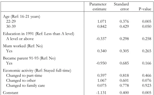
Table 2.1 presents the parameter estimates and standard errors for the linear regression of the change in gender role attitude on: age in 1991, categorised; highest educational qualification in 1991; whether mother worked when respondent was a child; and whether or not the woman became a parent between 1991 and 1993. The significant negative constant reveals that, on average, people between 16 and 21 years old become more traditional in their views. However,

9

the parameter estimates for those over 21 cancel this negative effect out, and hence the attitudes of the older groups do not change much. None of the other variables are significant.

Table 2.1: Parameter estimates for the linear regression of change in attitude between 1991 and 1993.

Parameter estimate

Standard

error P-value Age (Ref: 16-21 years)

22-29 1.071 0.376 0.005

30-39 0.842 0.429 0.050

Education in 1991 (Ref: Less than A level)

A level or above -0.337 0.298 0.258 Mum worked (Ref: No)

Yes 0.340 0.305 0.265

Became parent 91-93 (Ref: No)

Yes -0.950 0.685 0.166

Economic activity (Ref: Stayed full-time)

Changed to part-time 0.597 0.818 0.466 Changed to other 1.067 0.601 0.076 Changed to family care 0.075 0.778 0.923

Constant -1.131 0.400 0.005

A major draw back of the unconditional change score model is that the change is assumed to be independent of the response at the first time point given the predictor variables. In practice, this assumption is unlikely to hold. Indeed, initial status is frequently found to be negatively correlated with change, the so-called ‘regression to the mean’ effect (see, for example, Finkel 1995). An alternative model which does not make this assumption is the conditional change model, where the response at the first time point is included in the model as a predictor variable:

.

1 1 1 1 0 2 i p ip p i i i

x

x

y

e

Y

=

β

+

β

+

L

+

β

+

β

₊

+

_(1.1)

Note that it is usual to regress the response at the second time point on the predictors, rather than the change in response, since the two models are mathematically equivalent: subtracting the response at time 1 from both sides of equation (1.1) gives

,

)

1

(

_{1 1} 1 1 0 1 2 i i p ip p i i i

y

x

x

y

e

Y

−

=

β

+

β

+

L

+

β

+

β

₊

−

+

10

so the parameters for all the explanatory variables are unchanged and the parameter for the response at time point 1 is reduced by one. For further discussion concerning the merits of unconditional and conditional change score models see Finkel (1995). A major limitation of the change score model is that it can only be applied to two waves of data. Where we have more than two waves of data, this means the analyst must discard important information. In the following sections of the paper we consider models to analyse panel data that incorporate information from more than two waves of data.

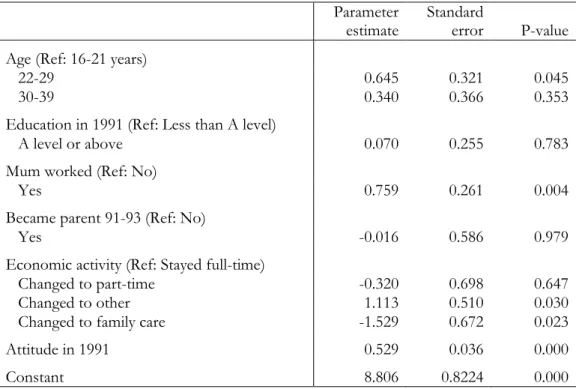
To illustrate the conditional change score model, Table 2.2 presents the parameter estimates and standard errors for the linear regression of attitude in 1993 on age, education, became parent, mum worked, economic activity and attitude in 1991 for the data set described above.

Table 2.2: Parameter estimates for the linear regression of attitude in 1993. Parameter

estimate

Standard

error P-value Age (Ref: 16-21 years)

22-29 0.645 0.321 0.045

30-39 0.340 0.366 0.353

Education in 1991 (Ref: Less than A level)

A level or above 0.070 0.255 0.783 Mum worked (Ref: No)

Yes 0.759 0.261 0.004

Became parent 91-93 (Ref: No)

Yes -0.016 0.586 0.979

Economic activity (Ref: Stayed full-time)

Changed to part-time -0.320 0.698 0.647 Changed to other 1.113 0.510 0.030 Changed to family care -1.529 0.672 0.023 Attitude in 1991 0.529 0.036 0.000

Constant 8.806 0.8224 0.000

Now after controlling for attitude in 1991, age is no longer significant. (The F-test that both parameters are zero gives F = 2.10, with p-value = 0.1239.) However, mother worked and economic activity are now significant, with those who mother worked when the respondent was

11

aged 14 becoming more liberal and those who took up family care between 1991 and 1993 becoming more traditional. The fact that change in economic activity becomes more significant in the conditional change model probably results from the association between age and change in economic activity and the association between age and initial gender role score.

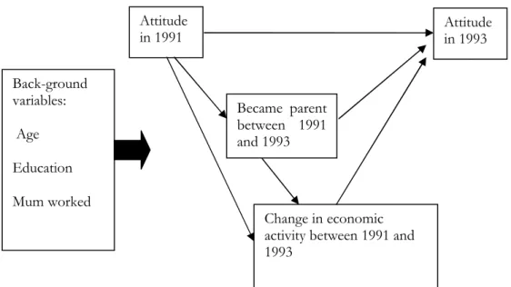
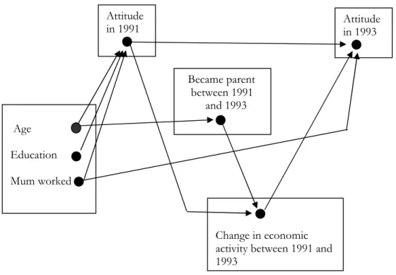
Thus far we have used the conditional change model to test some of the links in the conceptual framework presented in Figure 1.1: it has been used to identify the predictors of (change in) attitude in 1993, after controlling for attitude in 1991. We suspect however, that the conditional change model is overlooking important pathways for example through which gender role attitudes are associated with becoming a parent, and through which becoming a parent is associated with change in labour force status. We suspect that becoming a parent and change in economic activity are highly associated. By looking at the pathways in more detail using a graphical chain model we can identify whether gender role attitudes select individuals into parenthood, or are associated primarily with changes in economic activity. This is the topic of the next section.

Figure 1.1: Conceptual Framework for the Relationship between Attitude Change and Behaviour Change. Attitude in 1993 Back-ground variables: Age Education Mum worked Attitude in 1991 Became parent between 1991 and 1993 Change in economic activity between 1991 and 1993

12

3 GRAPHICAL CHAIN MODELS

Graphical models and graphical chain models are powerful tools to investigate complex systems consisting of a large number of variables (Wermuth and Lauritzen 1990). The graphical chain modelling approach builds up a complex model using a sequence of regression models. The use of linear, binary and multinomial logistic regression models allows the inclusion of continuous (e.g., attitude), binary (e.g., becoming a parent) and categorical (e.g., economic activity) responses. Below we introduce the mathematical graphs used in graphical modelling and review some of the key ideas of graphical modelling. For further details of the method see, for example, Whittaker (1990) or Cox and Wermuth (1996); for medical applications see Hardt et al. (2004) or Ruggeri et al. (2004); and for demographic applications see Mohamed, Diamond and Smith (1998), Magadi et al. (2004) or Borgoni, Berrington and Smith (2004).

3.1 Mathematical Graphs

A mathematical graph consists of a set of nodes (vertices) and a set of edges. Two nodes connected by an edge are called adjacent. The edge can be directed (also called an arrow) or undirected. A path is a sequence of adjacent nodes. A graph is acyclic if it does not contain any directed cycle, a directed cycle being defined as a path from a node back to itself following a directed route, i.e., a direction preserving path. Figure 3.1a shows an undirected graph with nodes labelled a, b, c, d and undirected edges (a, b), (a, c), (a, d) and (b, c). The sequence of nodes a, b, c

identifies one possible path from a to c. If the undirected edge from a to c is replace by an arrow then we have a cyclic graph as now the direction preserving path a, b, c, a is a path from a back to itself following a directed route. A subset of nodes C separates a subset of nodes A from a subset of nodes B if every path from a node in A to a node in B must pass through C. For example, in Figure 3.1a, the set C = {a} separates A = {b, c} from B = {d}.

13

Figure 3.1: (a) An acyclic graph (b) A chain graph.

(a) (b) a • b • a • b • • c • c • d • d

A chain graph is obtaining by partitioning the set of nodes in subsets called blocks. If nodes in different blocks are connected then this is by arrows, while if they are in the same block then they are connected by undirected edges. This block formulation excludes graphs with cycles. Nodes belonging to the same block are usually gathered into a box. Figure 3.1b shows a simple 2-block chain graph. A chain graph for which each block contains just one node is called a direct acyclic graph (DAG). However, a chain graph is more general than a DAG since it can contain a mixture of directed and undirected edges.

3.2 Graphical Models

Here nodes represent random variables and undirected edges the association between pairs of variables. A usual notation is to use circles for continuous variables and dots for categorical or nominal variables. Asymmetric relationships between variables, i.e., one anticipates in some sense the other, are represented by arrows. Figure 3.2a depicts a hypothetical graphical model, including three variables from our current example, containing interactions between age and education, age and mum worked and finally education and mum worked. Figure 3.2b displays a two block graphical chain model. A direction preserving path in a chain allows the representation of both direct and indirect effects. In Figure 3.2b for instance it is possible to identify a direct effect of education on attitude, as well as an indirect effect of mum worked through education.

14

Figure 3.2: (a) a graphical model and (b) a chain graph.

(a) (b) Age • Education • Age • Education • • •• • Mum worked •••• Mum worked • •• • Attitude

Fundamental to graphical modelling is the concept of conditional independence. A graphical model uses a graph to represent a set of conditional independence relationships amongst the corresponding variables. In particular, in an undirected (conditional) independence graph an edge between nodes a and b is missing if and only if Ya is independent of Yb given the remaining

variables under consideration. For example, in Figure 3.1a, Yc is conditionally independent of Yd

given Ya and Yb, since there is no edge between c and d, but Ya is not conditionally independent

of Yb given Yc and Yd, since there is an edge between a and c. An independence graph defined

in this way is said to satisfy the pairwise Markov property.

Under mild conditions, an independence graph also satisfies the global Markov property which means that any two subsets of variables which are separated by a third are conditionally independent give only the variables in the third subset. This result allows us to determine the conditional independence structure of subsets of the variables from the independence graph. For example, in Figure 3.1a Yc is also conditionally independent of Yd given just Ya, since C = {a}

separates A = {b, c} from B = {d}.

Defining the Markov properties of a chain graph is less straightforward; for details see, for example, Whittaker (1990) or Cox and Wermuth (1996). However, the following two rules based on the Markov properties are often helpful for drawing conclusions from a chain graph:

15

1. any non-adjacent pairs of variables (i.e., not joined by an edge) are conditionally independent given the remaining variables in the current and previous blocks;

2. a variable is independent of all the remaining variables in the current and previous blocks after conditioning only on the variables that are adjacent.

For instance, for the graph in Figure 3.2b it follows from rule 1 that attitude is independent of age given education and mum worked. From rule 2, it follows that attitude is independent of age and mum worked given the education, i.e., age and mum worked are only indirectly associated with attitude. Such variables are called indirect explanatory variables by Cox and Wermuth (1996).

A chain graph is a well recognised tool to specify causal relationships amongst processes (Pearl 1995). A chain graph drawn with boxes is viewed as a substantive research hypothesis about direct and indirect relation amongst variables (Wermuth and Lauritzen 1990). The variables are ordered a priori, as shown, for example, in Figure 3.2b. The model is specified according to theory which may suggest associations or dependencies to be omitted from the graph. The presence of an edge or an arrow in the graph can then be empirically tested. However, whilst we are able to demonstrate associations consistent with hypothesized causal links we are unable, when fitting chain graphs to observational data, to prove causality. Graphical chain models are ideally suited to situations where we have prospective data collected in sweeps of a panel survey. The temporal ordering of the data helps in identifying the causal ordering of variables across the life course. Also, graphical chain modelling can help cope with attrition as the available sample can be used in each stage of the chain, confining the potentially serious effect of drop-out to the later components of the chain.

16

3.3 Example: Graphical Chain Modelling of Women’s Gender Role Attitudes, Entry into Parenthood and Change in Economic Activity.

Following the conceptual framework in Figure 1.1, we use a graphical chain graph to examine the reciprocal relationship between gender role attitudes, entry into parenthood and change in economic activity among a sample of women who are initially childless and in full-time employment. We make the assumption that entry into parenthood precipitates a change in economic activity. (Although we are aware for that a minority of women, e.g., those experiencing redundancy, change in employment status could theoretically precipitate the ‘decision’ to have a child.) Whether the woman made a transition between 1991 and 1993 in her employment status is coded as a categorical variable (stayed full-time, moved to part-time, moved to family care, moved to other: retired, sick, unemployment, student).

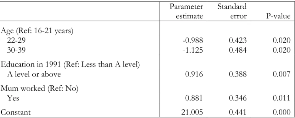
We have already modelled the predictors of attitude in 1993 (Table 2.2). Table 3.1 presents the parameter estimates and standard errors for the linear regression of attitude in 1991 on age, education and mum worked. Here we see that, on average, those aged between 16 and 21 were more liberal in 1991 than the other two groups. This helps explain the difference in the significance of age in the unconditional and conditional scores: those aged between 16 and 21 tend to have higher attitude scores in 1991 and change in score is related to attitude in 1991, so once ones controls for the initial score, age is not significant in the change score model. We also see from Table 3.1 that more educated women and women whose mother worked when the respondent was 14 are significantly more liberal.

17

Table 3.1: Parameter estimates for the linear regression of attitude in 1991. Parameter

estimate

Standard

error P-value Age (Ref: 16-21 years)

22-29 -0.988 0.423 0.020

30-39 -1.125 0.484 0.020

Education in 1991 (Ref: Less than A level)

A level or above 0.916 0.388 0.007 Mum worked (Ref: No)

Yes 0.881 0.346 0.011

Constant 21.005 0.441 0.000

A binary logistic regression model is used to investigate the predictors of becoming a parent. The parameter estimates of this model are presented in Table 3.2 and reveal that, for our childless sample, the odds of becoming a parent in the subsequent two years increase with age. An interaction between age and education is to be expected (Rendall and Smallwood 2003). However, given the small sample size, this interaction is not significant in our model (likelihood ratio test statistic = 3.91 on 2 degrees of freedom, p-value = 0.142), although the parameter estimates are in the right direction: aged between 16 and 21, more educated women have lower odds of becoming a parent compared to the less educated, but when aged between 30 and 39 they have higher odds.

Table 3.2: Parameter estimates for the logistic regression of becoming a parent between 1991 and 1993.

Parameter estimate

Standard

error P-value Age (Ref: 16-21 years)

22-29 1.014 0.434 0.019

30-39 1.016 0.470 0.031

Education in 1991 (Ref: Less than A level)

A level or above -0.171 0.273 0.531 Mum worked (Ref: No)

Yes 0.467 0.297 0.115

Attitude in 1991 -0.032 0.038 0.392

18

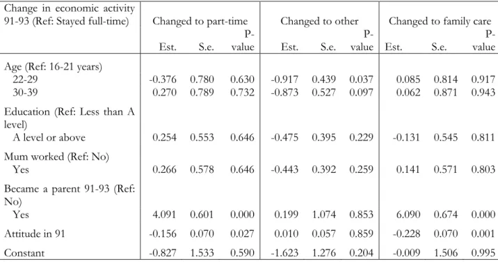
A multinomial logistic regression model is used to investigate the predictors of change in economic activity. The parameter estimates of this model are presented in Table 3.3 and reveal that the odds for moving to part-time work or family care, compared with staying full-time, are greatly increased if the woman becomes a parent. Attitude in 1991 is also a significant predictor. Women with more liberal attitudes are more likely to remain in full-time work and less likely to change to part-time or to take up family care. Likelihood ratio tests reveal that overall, none of the other variables are significant.

Table 3.3: Parameter estimates for the multinomial logistic regression of change in economic activity between 1991 and 1993.

Change in economic activity

91-93 (Ref: Stayed full-time) Changed to part-time Changed to other Changed to family care Est. S.e.

P-value Est. S.e.

P-value Est. S.e.

P-value Age (Ref: 16-21 years)

22-29 -0.376 0.780 0.630 -0.917 0.439 0.037 0.085 0.814 0.917 30-39 0.270 0.789 0.732 -0.873 0.527 0.097 0.062 0.871 0.943 Education (Ref: Less than A

level)

A level or above 0.254 0.553 0.646 -0.475 0.395 0.229 -0.131 0.545 0.811 Mum worked (Ref: No)

Yes 0.266 0.578 0.646 -0.443 0.392 0.259 0.141 0.571 0.803 Became a parent 91-93 (Ref:

No)

Yes 4.091 0.601 0.000 0.199 1.074 0.853 6.090 0.674 0.000 Attitude in 91 -0.156 0.070 0.027 0.010 0.057 0.859 -0.228 0.070 0.001 Constant -0.827 1.533 0.590 -1.623 1.276 0.204 -0.009 1.506 0.995

We summarize the results graphically (Figure 3.3). From Rule 1, the absence of an edge between attitude in 1993 and becoming a parent 1991 and 1993 indicates that they are conditionally independent given the variables in the preceding blocks. From Rule 2 we conclude that attitude in 1993 is independent of age, education and becoming a parent, given attitude in 1991, whether the respondent’s mother worked and change in economic activity. Hence, change in gender role attitude is not associated with becoming a parent per se, but with the move to part-time work or

19

family care that often accompanies first motherhood. The graph also tells us that entry into parenthood is independent of gender role attitudes, given the other variables in the preceding blocks, but that change in economic activity is dependent upon gender role attitudes. Finally, the chain graph tells us that age is only indirectly associated with attitude change, for example, through its impact on initial attitude and on the likelihood of becoming a parent.

Figure 3.3. Graphical chain graph of women’s gender role attitudes, entry into parenthood and change in economic activity.

A disadvantage of our graphical chain model is that it assumes that gender role attitude is measured without error. A more sophisticated approach would be to estimate gender role attitude as an underlying latent variable, regressed on six indicator variables (the attitude statements). Panel data where we have repeated measurement of a multiple indicator latent construct over time can provide useful information about the magnitude of measurement error and opportunities for estimating models which take account of measurement error. For this to be possible however, we need an approach which estimates all of the regression equations simultaneously, and a global measure of model fit. Structural equation models, which have these

Attitude in 1993 Age Education Mum worked Attitude in 1991 Became parent between 1991 and 1993 Change in economic activity between 1991 and 1993

20

capabilities and hence can include correlated errors of measurement and correlated structural disturbances terms, are the subject of Sections 4 and 6.

21

4 CROSS-LAGGED STRUCTURAL EQUATION MODELS

If we are interested in the nature of the relationship between two variables,

X

and

Y

, four possible causal systems could underlie the covariance structure of the observed data, assuming both

X

and

Y

are not influenced by any third variable,

Z

:

X

does not cause

Y

and

Y

does not cause

X

;

X

causes

Y

and

Y

does not cause

X

;

Y

causes

X

and

X

does not cause Y;

X

causes

Y

and

Y

causes

X

.

A cross-sectional regression of

Y

on

X

, or

X

on

Y

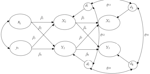
, will only enable the analyst to discount the first of these possibilities, by rejecting the null hypothesis of zero correlation at the specified level of confidence. Where zero correlation can be rejected as unlikely, given the sample data, any of the three remaining possibilities could still represent the true data generating mechanism in the population.

Cross-lagged structural equation models (Finkel 1995; Marsh and Yeung 1997; Campbell and Kenny 1999) make use of the inherent time ordered nature of panel data to address such questions of causal ordering. Cross-lagged models are also known as ‘simplex models’, ‘autoregressive models’, ‘conditional models’ and ‘transition models’ (Twisk 2003). A definitional feature of this type of model is that it is estimated in a single step, rather than as a series of separate regressions. An advantage of the single estimation is that it yields a global likelihood for the model and, thereby, the full range of tests and indices of model fit that are standard within the SEM framework (Bollen 1989). The basic structure of the cross-lagged model is presented in Figure 4.1, which shows a path diagram for a three wave, two variable cross-lagged panel model.

22

Figure 4.1: Three wave, two variable cross-lagged panel model.

Here there are two variables of interest,

X

and

Y

, and each variable (represented by ellipses in Figure 4.1) is regressed on both its own lagged score and the lagged score of the other variable at the previous measurement occasion. At the first wave of measurement,

x

1 and

y

1 are specified

as exogenous and allowed to covary. An alternative specification of this model is for the cross effects to be synchronous, that is running between

X

and

Y

variables at the same time point, as opposed to the lagged measure. This specification may be preferred where the time gap between measurements is long and when the proposed causal mechanism is of short duration, although it can raise identification and estimation problems not found in the cross-lagged model.

The model in Figure 4.1, then, provides an estimate of the (lagged) effect of each variable of interest on the other, net of autocorrelation of each variable with its lagged measurement, and whatever additional covariates are included in the model. The model parameters of greatest interest in the cross-lagged model are the auto-regressive (

β

1

,

β

4

,

β

5

,

β

8) and cross-lagged

(

β

2

,

β

3

,

β

6

,

β

7) regression coefficients. The auto-regressive parameters, in conceptual terms,

determine the stability of the rank ordering of individuals on the same variable over time. The cross-lagged regression parameters, on the other hand, tell us how much variation in one variable

y1 ρ12 β7 β5 β6 1

x

β1 β2 β3 Y2 ρ24 ρ13 X3 ρ34 X2 d1 d2 d₃ d₄ Y3 β4 β8

23

at time

t

1 is able to predict change in the other variable between times

t

1 and

t

2, net of any

controls specified in the model. For example, if we find positive and significant cross-lagged coefficients running in both directions, this supports a reciprocal effects model, in which each variable exerts a causal influence on the other over time. If only one of the cross-lagged coefficients is statistically significant, we can conclude that the causal relationship is uni-directional in nature. If neither of the cross-lagged coefficients are significant, we should infer that the two variables are causally unrelated. Note that the inclusion of a lagged endogenous variable provides some ‘protection’ against the effects of unobserved time-constant variables. However, unlike the fixed effects models discussed in Sections 5 and 6, the lagged endogenous variable approach cannot completely remove unobserved unit heterogeneity (Halaby 2004; Allison 2005).

The general structure presented in Figure 4.1 can be extended to include multiple variables and multiple waves of data (see Finkel 1995). The coefficients for the stability and lagged effects may, respectively, be constrained to equality across waves, making these parameters equivalent to ‘average’ effects over the duration of the panel. Although applying this type of equality constraint does not provide a solution to the problem of mapping discrete measurement intervals on to continuous processes, it can give a longer and, therefore, more realistic time frame over which to examine the hypothesised relationships. The empirical adequacy of such equality constraints can be assessed via the likelihood ratio test, against the unconstrained model, as these are nested one within the other. Where no loss of fit is incurred by fixing these parameters to equality over time, the constrained model should generally be preferred.

4.1 Correlated Disturbance Terms

An important thing to note about cross-lagged models is the importance of modelling covariances between the disturbances (represented by circles

d

1 to

d

4 in Figure 4), both within

24

of endogenous variables in the model and there are often good reasons to expect positive correlations between them. If, for example, a third variable, Z, causes both endogenous variables

X

2 and

Y

2 but Z is not included in the model, the disturbance terms of

X

2 and

Y

2

will necessarily be correlated (Anderson and Williams 1992). Similarly, we might expect to observe a positive correlation between the disturbances of the same lagged endogenous variable over time, resulting from a stable un-modelled cause of the variable in question (Williams and Podsakoff 1989). Failing to estimate covariances between disturbance terms can lead to biased estimates of cross-lagged and stability parameters and is a major reason for preferring this type of model over those which proceed via a series of independent, local estimations and hence, in practice, fix these covariances at zero.

4.2 Measurement Error Models

The model set out in Figure 4.1 implicitly assumes that the variables of substantive interest are measured without error. This is not a realistic assumption and, in practice, the vast majority of survey items are likely to contain both random and systematic components of error. This results from, inter alia, imperfections in the wording and layout of questionnaires, the personality and mood of the respondent and the mode in which the interview is conducted.

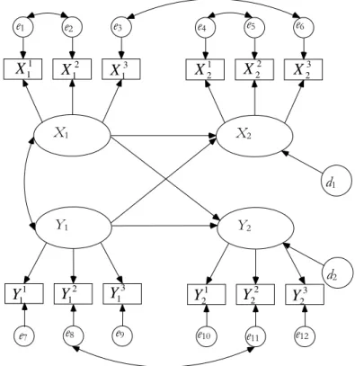
Measurement error in independent variables results in attenuated effect sizes, so models which make a correction for measurement error are more likely to detect effects that are real, but possibly weak, in the population (Bollen 1989). In autoregressive models, systematic measurement error that is stable over time will manifest in the form of upwardly biased stability estimates for the concept of interest. Figure 4.2 shows a path diagram for a two variable, two wave, cross-lagged panel model with error correction and modelled error covariances.

25

Figure 4.2: Cross-lagged model with measurement error correction.

Each of the concepts of analytical interest (

X

and

Y

) are specified as latent variables measured by three observed indicators, shown as rectangles in Figure 4.2 (X11 to

3 2 X and Y11 to 3 2 Y ).

Each observed variable has an associated error variance, denoted by circles labelled

e

1 to

e

12 in

Figure 4.2. The model partitions the variance of each observed variable into that which is caused by the latent variable of interest and that which is error (both systematic and random). The analyst can then specify covariances between the error terms, where they are expected or indicated post hoc, through indicators of model fit. In Figure 4.2 a covariance path is estimated between the error terms of the first and second indicators of latent variable

X

at each wave (denoted by the curved double-headed arrow between them). Similarly, covariances between the error terms of the same item over the two waves of measurement are estimated for the third indicator of latent variable

X

and the second indicator of latent variable

Y

. Another way of treating covariances between error terms is to model them directly as indicators of higher order latent variables or method factors (Rigdon 1994), though a consideration of this approach is beyond our scope here.

X1 1 1 X e1 2 1 X e2 3 1 X e3 X2 1 2 X e4 2 2 X e5 3 2 X e6 Y1 3 1 Y e9 2 1 Y e8 1 1 Y e7 Y2 3 2 Y e12 2 2 Y e11 1 2 Y e10 d1 d2

26 4.3 Factorial Invariance

A further benefit of the use of multiple indicators is that measurement invariance over time may be evaluated. The problem, generally stated, is that questions may change their meaning over time, rendering estimates of stability and change inferentially problematic. While it is clearly not possible to impose invariant meaning on survey questions through any statistical procedure, it is possible to impose such a constraint and then test its reasonableness through standard measures of model fit (Meredith 1993). Measurement invariance can be imposed by constraining the corresponding factor loading between the latent variable and observed variables to equality at each time point. For example, in Figure 4.2, we would constrain the loading between

X

1 and

1 1

X to be equal to the loading between

X

2 and 1 2

X , and so on. A likelihood ratio test can then be performed to test the null hypothesis of no change in the relationship between the latent variable and its indicators over time. This kind of test is not available for single indicator or composite variables and any measurement invariance would be incorrectly identified as change in the underlying concept using these types of measure.

4.4 Example: Economic Values and Economic Perceptions

In this example, we fit a series of cross-lagged models to investigate the relationship between retrospective perceptions of the macro economy (EP) and ‘left-right’ economic values (EV). The data come from the British Election Panel Survey 1992-1997. The first wave of the study was conducted in April 1992 with a response rate of 73%, representing a total sample size of 3534. Respondents were then followed up annually until 1997 using a combination of face-to-face, telephone and postal methods. The analytical focus for this study comprises those individuals who were interviewed in 1992, 1994, 1996 and 1997, which due to attrition reduced the analytical sample to 1640 respondents. EP is measured by three five point items tapping perceptions of the unemployment rate, the rate of taxation, and the general standard of living ‘since the last election’ (1992). EV is measured by the six item scale developed by Heath, Evans and Martin (1993), the full question wordings of which can be found in Appendix A.

27

In the models that follow, we use either summed scale or latent variable measures of each construct. Both approaches can be viewed as a form of error correction, although the latent variable approach involves a more robust correction and allows modelling of covariances between error terms. We specify no strong hypotheses regarding the causal relationships between these two variables. However, we note that a plausible case can be made for each to cause the other. To wit, economic perceptions have been shown to be partially endogenous to political preferences (Evans and Andersen 2006) and beliefs about how the economy should be managed may be influenced by an individual’s assessment of macro-economic performance (e.g., government fiscal policy should vary as a function of the rate of inflation and the jobless count).

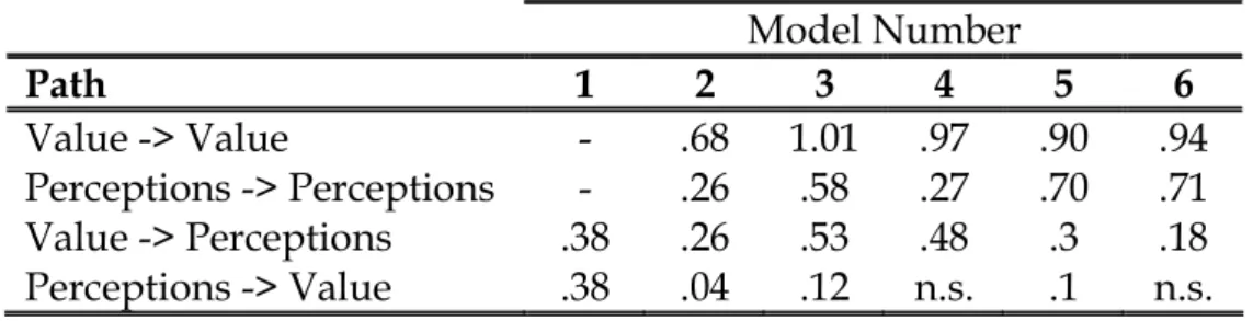
The models we present are deliberately selected to demonstrate the importance of two issues in model specification discussed above: correcting for random and systematic errors in the measurement of concepts; and specifying an appropriate covariance structure between error and disturbance terms. Our data source for the following analyses is the 1992 to 1997 British Election Panel Study, covering five waves of data collection (the economic perception variables were not administered in 1993), with an analytical sample size of 1640. Table 4.1 presents a summary of the estimated standardised regression coefficients for each model, fitted using MPlus 3.1 (Muthén and Muthén 2003).

Table 4.1: Summary of cross-lagged and auto-correlated parameter estimates

Model Number

Path

1

2

3

4

5

6

Value -> Value

-

.68

1.01

.97

.90

.94

Perceptions -> Perceptions

-

.26

.58

.27

.70

.71

Value -> Perceptions

.38

.26

.53

.48

.3

.18

Perceptions -> Value

.38

.04

.12

n.s.

.1

n.s.

28

We begin by fitting a ‘naïve’ model (Model 1), which simply regresses the 1992 cross-sectional summed-scale measure of EP on to the 1992 cross-sectional summed-scale measure of EV. We find a significant positive relationship of 0.38. Because this is a cross-sectional regression, the standardised estimate of the causal influence of EP on EV is the same as that of EV on EP and the observed association may not be indicative of a causal relationship. Next, in Model 2, we make use of the longitudinal dimension of the data by fitting a cross-lagged panel model to the first two waves of data (1992 and 1994), again using the summed scale measures of each concept. The covariance between the disturbances of the two endogenous variables is not estimated. The results of this model suggest a reciprocal mechanism, with significant cross-lagged effects in both directions, although both coefficients are considerably weaker than those from the ‘naïve’ cross-sectional model, with the path running from EP to EV now only marginally greater than zero.

Model 3 replicates Model 2, but this time each concept is specified as a latent variable, measured by multiple indicators. No covariance paths between error terms of the observed variables or disturbances of the endogenous variables are estimated. The parameter estimates for Model 3 show a marked increase in magnitude, as would be expected after a correction for random error in the independent variables. Model 4 estimates covariances between the error terms for the same item over time, in order to accommodate systematic error in the indicators of the latent constructs. This has the effect of reducing the magnitude of the estimates of the cross-lag and stability parameters. Again, this should be expected, because in the previous model these systematic errors have effectively been channelled into the stability and cross-lagged parameters. Note, also, that in Model 5 the path from economic perceptions to economic values now becomes non-significant. Model 5 extends Model 4 to incorporate all five waves of data. The coefficients for the stability and lagged effects are constrained to be equal across waves. Factor loadings for the same item are constrained to equality across waves to impose meaning invariance on the items as measures of the latent concepts. By extending the model over 5 waves of data again we have changed the nature of the causal inference; we now find support for the reciprocal effects model, with both cross-lagged paths positive and significant at the 5% significance level.

29

Model 5, however, constrains the covariances between the disturbance terms of the endogenous variables to zero. Model 6 freely estimates the covariances between adjacent disturbance terms for the same endogenous variable and between the disturbance terms for the two endogenous variables at the same wave of measurement. This has the effect of making the causal path from EP to EV non-significant and indicates that the apparent causal effect for this parameter, identified in earlier models, likely results from un-modelled causal variables. In summary, this example demonstrates how different approaches to modelling error the variances and covariances can substantially alter the nature of the causal inferences an analyst would make.

30

5 RANDOM EFFECTS MODELS FOR REPEATED MEASURES DATA

Both graphical chain models and cross-lagged panel models can be used to model the pathways through which variables measured over time are associated. However, both frameworks model the repeated measures as a set of discrete transitions from one time point to the next. Often we are interested in addressing a rather different set of questions about change over time, which treat the repeated measures as a sample of observations taken from a continuous developmental process. For example, imagine that we have 12 weight measurements taken from a sample of newborns at monthly intervals. Rather than analysing the data as a chain of regressions of each time point on the previous measurement (or some other lag function), we might wish to model the repeated observations as indicators of an underlying developmental trend. For this example, we would expect the overall trend (weight in newborns) to be broadly linear and positive (most children grow steadily over the first year of life). However, we would also expect there to be some individual variation around this overall trend, with some children growing faster than others. If individuals do vary in their rates of growth, we will naturally be interested in understanding the characteristics of individual children (both time-constant and time-varying) that are associated with variability in growth. It is these types of questions that random effects models are well suited to addressing. Random effects models, also called multilevel models, are discussed in detail in the books by Hox (2002) and Snijders and Bosker (1999).

A naïve model for a linear trend over time would be the simple linear regression model of the response on time:

.

1 0 ij ij ij

t

e

Y

=

β

+

β

+

(5.1)

If we can assume that the errors

e

ij have mean zero and are independent for different

i

or

j

,

then we can use standard methods to fit this model. However, for repeated measures of the response on the same individual, it is unlikely that

e

ij is independent of

e

ik, for

j

≠

k

, that is, it

is unlikely that the errors are uncorrelated over time, even if we were to add covariates to the model (5.1).

31

To address this problem, consider the alternative model

,

1

0 ij i ij

ij

t

u

e

Y

=

β

+

β

+

+

(5.2)

where

u

i is the individual-specific residual and represents unmeasured individual factors which

affect

Y

.

A random intercept model, which enables the analyst to model individual trajectories of development over time, specifies that

u

_i follows a normal distribution with mean zero and

variance

σ

_u2. Furthermore, it is assumed that

u

_i is uncorrelated with

e

_ij and

t

_ij. Under this

assumption it follows that the variance of

Y

ij is

,

2 2

e

u

σ

σ

+

where

σ

_u2 measures the

between-individual variation and

σ

e2 is the residual within-individual variation. Hence, the proportion of

the total variation that can be attributed to the between-individual variation is

.

2 2 2 e u u

σ

σ

σ

ρ

+

=

This ratio is also the within-individual correlation, often called the intra-class correlations. If most of the variation is between individuals then individuals change little over time and hence the intra-class correlation is large. Conversely, if there is a lot of variability within individuals (relative to the total variability) then the intra-class correlation will be small. See Snijders and Bosker (1999) and Hox (2002) for basic introductions to the random intercept model and interpretation of

ρ

.

The random intercept model (5.2) can be extended in two ways. (1) Time-constant and time-varying covariates can be added to explain some of both the within and between individual variation. (2) Different, or more complicated functions of time can be used in the model. For example, if the response did not vary linearly with time, then time could be replaced by log(time) or a time-squared could be added to the model. Where there is no a priori theoretical expectation for the shape of the trajectory, one approach for selecting an appropriate growth function is to

32

inspect the empirical growth record for the sample as a whole (Willett and Sayer 1994). Another is to start by including time as a factor in the model and then to examine the estimated effects at each time points for trends. This is the approach we use in our example below.

The random intercept model assumes that the correlation between any two responses for the same individual is the same and equals

ρ

.

For example, this model assumes that the correlation between the first and last observation on an individual is the same as the correlation between the first and second observations. The correlation structure is often called exchangeable or uniform and is often untenable when there are more than a few repeated observations on each individual.

One way to relax the assumption of an exchangeable correlation structure is to allow the coefficient of time to also vary randomly across the individuals by including a random slope for time:

.

)

(

₁ 0 i ij i ij ij

b

t

u

e

Y

=

β

+

β

+

+

+

(5.3)

Here

b

i is an individual specific normally distributed random slope with mean zero and variance 2

b

σ

. Furthermore,

b

i is assumed to be uncorrelated with

e

ij but can be correlated with

u

i.

Unlike the random intercept model, the random slope model does not impose an exchangeable correlation structure on the data and the variance of

Y

_ij is not constant over time.

5.1 Example: Random Effects Modelling of Men’s and Women’s Gender Role Attitudes Over Time

Our aim is to examine the factors related to men’s and women’s gender role attitude score, as measured in 1991, 1993, 1995 and 1997. The data come from the British Household Panel Survey. Men and women aged 16 to 59 who were childless in 1991 and who took part in all of the waves through to 1997 are taken as the analysis sample of 1429 individuals. A summary score of gender role attitude is derived as the sum of the responses to six attitude statements (see

33

Appendix A), with the repeated measure of gender role attitude nested within individuals. Therefore we have individuals i = 1 to 1429 and observations j = 1 to 4, for all individuals. Our dependent variable is the summed attitude score at observation j for individual i, Yij at

t

ij

,

= 1 i

t 1991, …, ti4=1997. Our covariates are: sex; age in 1991, categorized; highest educational

qualification in 1991; whether the respondent’s mother worked when she was a child; and current economic activity, which is time-varying.

The responses to the attitude statements at different time points on the same individual are unlikely to be independent, even after conditioning on the covariates. Therefore, we take account of this by partitioning the total residual for individual

i

at time point

j

into an

individual-specific random intercept

u

i which is constant over time, plus a residual

e

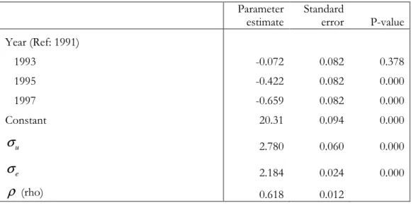
ij which varies

randomly over time. First, let us consider time as a factor and no other covariates. Three dummy variables are included in the model to indicate whether the observation was taken in 1993, 1995 or 1997. (The reference group is 1991.) Table 5.1 presents the maximum likelihood estimates of the parameters in this model. From these estimates, we can see that score decreases with time and so henceforth we consider time as a continuous variable; see Table 5.2.

Table 5.1: Parameter estimates for random-intercept linear regression of attitude with time included as a factor. Parameter estimate Standard error P-value Year (Ref: 1991) 1993 -0.072 0.082 0.378 1995 -0.422 0.082 0.000 1997 -0.659 0.082 0.000 Constant 20.31 0.094 0.000 u

σ

_{2.780 0.060 0.000} e

σ

_{2.184 0.024 0.000}

ρ

(rho) _{0.618 0.012}

34

Table 5.2: Parameter estimates for the random-intercept linear regression of attitude with time treated as continuous. Parameter estimate Standard error P-value Time -0.116 0.013 0.000 Constant 20.374 0.088 0.000 u

σ

_{2.780 0.060 0.000} e

σ

_{2.185 0.024 0.000}

ρ

_{0.618 0.012}

The magnitudes of the estimates of the between-individual and the within-individual standard deviations,

σ

_u and

σ

_e respectively, are similar suggesting that, after controlling for time, there is unexplained variation in gender role attitudes both between individuals and within individuals over time.

Next we include main effects for the remaining covariates (Table 5.3). All of the covariates are found to be significantly associated with gender role attitude. Positive parameter estimates indicate a higher attitude score. Hence, more liberal attitudes are found, on average, if the individual is female, younger, more educated, if their own mother worked when they were a child, and if they work full-time. More conservative attitudes are found among those undertaking family care.

35

Table 5.3: Parameter estimates for the random-intercept linear regression of attitude with time and the other covariates.

Parameter estimate

Standard

error P-value

Time -0.101 0.013 0.000

Sex (Ref: Male) 1.254 0.151 0.000 Age (Ref: 16-21 years)

22-29 -0.579 0.183 0.002

30-39 -0.736 0.209 0.000

40-59 -1.653 0.292 0.000

Education in 1991 (Ref: Less than A level)

A level or above 0.544 0.152 0.000 Mum worked (Ref: No)

Yes 1.045 0.1544 0.000

Economic activity (Ref: Full-time)

Part-time -0.517 0.152 0.001 Other -0.303 0.108 0.005 Family care -1.883 0.193 0.000 Constant 18.24 0.289 0.000 u

σ

_{2.566 0.057 0.000} e

σ

_{2.170 0.023 0.000}

ρ

_{0.583 0.012}

The inclusion of individual-specific characteristics, such as sex age and economic activity, has reduced

σ

_u from 2.780 to 2.566 and

σ

_e from 2.185 to 2.170. In other words the covariates in the model are able to explain some of the between-individual differences, and only a little of the within-individual variability over time. We have only included one time-varying covariate: economic activity. We might speculate that the inclusion of more time-varying covariates would result in a greater ability to explain more of the within-individual variability.

By including interactions between each covariate and time we can test whether the impact of any of the covariates on gender role attitude changes over time. Interactions of time with age and economic activity were non-significant (confirmed using likelihood ratio tests) and so were

36

removed. The parameter estimates for the resulting final model are shown in Table 5.4. The results suggest that gender role attitudes decrease, in comparison with the baseline men’s scores, if the individual is a woman, is more educated, and if their mother worked.

Table 5.4: Parameter estimates for the random-intercept linear regression of attitude with time, the other covariates and significant interactions between time and the other covariates.

Parameter estimate

Standard

error P-value

Time 0.020 0.027 0.459

Sex (Ref: Male) 1.488 0.169 0.000 Sex by Time interaction -0.081 0.026 0.002 Age (Ref: 16-21 years)

22-29 -0.579 0.183 0.002

30-39 -0.736 0.209 0.000

40-59 -1.653 0.292 0.000

Education in 1991 (Ref: Less than A level)

A level or above 0.755 0.171 0.000 Education by Time interaction -0.070 0.026 0.007 Mum worked (Ref: No)

Yes 1.279 0.174 0.000

Mum worked by Time interaction -0.078 0.026 0.003 Economic activity (Ref: Full-time)

Part-time -0.451 0.152 0.003 Other -0.289 0.108 0.008 Family care -1.807 0.194 0.000 Constant 19.12 0.210 0.000 u

σ

_{2.569 0.057 0.000} e

σ

_{2.163 0.023 0.000}

ρ

_{0.585 0.012}

We can also include random coefficients or random slopes into our model to allow for between-individual heterogeneity in the effects of the covariates. Let us add a random coefficient (slope) for time to the model that includes all of the other main effects and interactions which were found to be significant in the random intercept model (Table 5.5).

37

Table 5.5: Parameter estimates for the random-effects linear regression of attitude with time, remaining covariates and significant interactions between time and the remaining covariates.

Parameter estimate

Standard

error P-value

Time 0.020 0.031 0.512

Sex (Ref: Male) 1.486 0.172 0.000 Sex by Time interaction -0.084 0.029 0.004 Age (Ref: 16-21 years)

22-29 -0.582 0.183 0.002

30-39 -0.735 0.210 0.000

40-59 -1.648 0.292 0.000

Education in 1991 (Ref: Less than A level)

A level or above 0.758 0.174 0.000 Education by Time interaction -0.069 0.029 0.016 Mum worked (Ref: No)

Yes 1.280 0.177 0.000

Mum worked by Time interaction -0.078 0.030 0.003 Economic activity (Ref: Full-time)

Part-time -0.421 0.153 0.006 Other -0.272 0.108 0.012 Family care -1.691 0.195 0.000 Constant 19.12 0.213 0.000 b

σ

_{0.311 0020} u

σ

_{2.732 0.072}

Correlation between

u

i and

b

i -0.306 0.048

e

σ

_{2.008 0.027}

The random intercept coefficient is of a similar magnitude as before suggesting that there is significant unobserved individual-level variation in the initial attitude score. The random slope coefficient is 0.311 and statistically significant suggesting that there is also significant variation between individuals in the way attitudes change over time. The average slope across men is 0.020. However, this slope varies randomly between individuals with a standard deviation of 0.311. Therefore, a man whose slope is one standard deviation above the average has a slope of