Electronic copy available at: https://ssrn.com/abstract=2638485
1 | P a g e
Does Size Matter in Predicting
SMEs Failure?
Jairaj Gupta
Department of Finance, University of Birmingham Birmingham, B15 2TY, UK; email: [email protected]
Mariachiara Barzotto
Essex Business School, University of Essex
Colchester, CO4 3SQ, UK; email: [email protected]
Amir Khorasgani
School of Economics, Finance and Accounting, Coventry University Coventry, CV1 5FB, UK; email: [email protected]
June, 2018
Abstract
This study acknowledges the diversity between micro, small and medium-sized firms while predicting bankruptcy and financial distress of United States small and medium-sized enterprises. Empirical findings suggest that survival (failure) probability increases (decreases) with increasing firm size and firms in different size categories have varying determinants of bankruptcy, while factors affecting their financial distress are mostly invariant. Magnitude of significant covariates changes across the size categories of both bankrupt and financially distressed firms. Further, operating cash flow information does not add any marginal increment in prediction performance of multivariate hazard models above baseline models developed using information from income statements and balance sheets. This result holds for failure likelihood of SMEs as well as their respective size categories.
Keywords: bankruptcy; SMEs; survival analysis; financial distress; operating cash flow
JEL Classification Codes: G32; G33
Acknowledgements: The authors are sincerely grateful to the Editor and anonymous referees
for their insightful comments and suggestions that improved this paper significantly. An earlier version of this paper was circulated under the title “Bankruptcy and Financial Distress in US
Electronic copy available at: https://ssrn.com/abstract=2638485
2 | P a g e
1. Introduction
In developed economies, small and medium-sized enterprises (SMEs) are, relative to turnover, disproportionately linked to employment rates. In the United States (US), for instance, almost half of all employees work for enterprises with fewer than 250 employees. SMEs play a crucial role in the global economy, and are pivotal to the economic growth and development of a country (Bosma and Levie 2010), as well as to poverty reduction (Koshy and Prasad 2007). Therefore, a detailed understanding of the factors affecting SMEs survival is important for policy makers, firms and capital suppliers. The attention devoted to SMEs survival has constantly increased over the years, particularly after the financial crisis in 2008-09. Indeed, the revised Basel capital accords and national governments have placed greater emphasis on understanding the credit risk attributes of SMEs.
Notwithstanding the extensive literature on the performance and financial distress of SMEs, the factors and the extent to which they affect SMEs failure likelihood across size
categories are still overlooked. As argued in a recent study by Altman et al. (2017), bankrupt and non-bankrupt firms have different boundaries due to their size (small and large), which affect the accuracy of prediction when data from one size category is used for another size category. Building upon the previous evidence showing that size affects access to finance (e.g. Beck and Demirguc-Kunt 2006), we propose a development in modelling financial distress and bankruptcy in the US. More specifically, we address this issue by exploring whether insolvency and financial distress likelihood varies across size categories of the US SMEs, by looking at the factors affecting SMEs failure likelihood in three sub-categories of SMEs (namely, micro, small, and medium1). Few studies explore the differences amongst the sub-categories of SMEs. Analysing financial and non-financial factors affecting UK SMEs bankruptcy across company size, Gupta et al. (2015) show that the credit risk characteristics of micro firms significantly differ from SMEs as a whole. Accordingly, they suggest that they should be treated separately
1
This paper classifies SMEs into three size categories (micro, small, and medium firms) as defined by the latest European Union classification. According to this classification, a firm is considered ‘micro’ if it has less than 10 employees with an annual turnover of less than €2 million (about $2.6 million); ‘small’ if it has less than 50 employees with an annual turnover of less than €10 million (about $13 million); and ‘medium’ if it has less than 250 employees with an annual turnover of less than €50 million (about $65 million). Further information can be found at: http://ec.europa.eu/growth/smes/business-friendly-environment/sme-definition/index_en.htm (accessed on July 28, 2015).
Electronic copy available at: https://ssrn.com/abstract=2638485
3 | P a g e for better pricing of credit risk and devising effective credit policies. In the light of this discussion, we expect the default characteristics to vary across SMEs size categories. We draw upon and advance this study by: i) using firms’ annual sales turnover, which is a preferred/more appropriate proxy of firms’ size than number of employees; ii) providing distinct evidence for two default definitions: bankruptcy (based on Chapter 7/11 filings), and financial distress (based on a firm’s ability to honour its financial commitments, and the value of its net worth); iii) exploring operating cash flow marginal discriminatory power across size categories; and, iv) examining the presence of statistically significant differences in the magnitude of mutually significant covariates in the model for all SMEs, and models for respective size categories, via the statistical (Wald) test of equivalence of coefficients.
Based on our empirical analysis in the context of US SMEs, using annual firm level financial information obtained from the Compustat database (from 1990 to 2014), we conclude that all SMEs are not the same. More specifically, the determinants of bankruptcy vary across different size categories of SMEs. Earnings are only found to be important for the largest size category, as is also the case for the ratio of assets to liabilities. Financial expenses are almost always found to be significant, but the size of its effect varies, especially in reference to micro firms. We also present compelling evidence that estimated coefficients differ between models for financial distress estimated across SMEs as a whole, and the varying size categories. Forecasters would therefore be advised that distinct models for bankruptcy or financial distress should be specified not in reference to SMEs as a whole, but rather in consideration of the different size classifications. In contrast to the work by Gentry et al. (1987) and Gilbert et al.
(1990), we do not find that cash-flow contributes to an understanding of bankruptcy. However, the results do compliment the findings of Charitou et al. (2004) for the UK in explaining financial distress using cash flow from operations (CFO).
There are a number of differences in the estimated determinants of financial distress as opposed to bankruptcy. Firms with greater holdings of cash and short-term investments are less likely to face financial distress. Taxes are consistently found to have an effect on financial distress, but this is not the case for bankruptcy, where only the model across SMEs as a whole provides evidence of a significant effect. There is also evidence that the effect of the ratio of current assets to current liabilities is different across different classes of firm when predicting
4 | P a g e financial distress. The value of trade debt predicts financial distress, concordant with the findings of Hudson (1986) and Beck et al. (2006). It is possible that the value of trade credit is reduced as a firm appears more likely to file for bankruptcy, explaining the different result. Bankruptcy and financial distress are distinct events and separate modeling of them shall lead to improved risk pricing. A similar conclusion might be reached in reference to the consideration of different size categories of firms.
The remainder of the paper is structured as follows: Section 2 presents a literature review on bankruptcy prediction and survival analysis, which is the foundation for SMEs failure prediction analysis, and includes the potential effect of firm size and operating cash flow on SMEs likelihood of entering financial distress and bankruptcy. Section 3 outlines the empirical methods, including an explanation of the dataset and covariates. Results and discussion are reported in Section 4. Finally, Section 5 draws conclusions and policy implications.
2. Literature Review and Hypotheses Development
This section reviews the past studies on bankruptcy prediction and survival analysis and is the foundation for our SMEs failure prediction analysis. The discussion also includes the potential effect of firm size and operating cash flow on SMEs likelihood of entering financial distress and bankruptcy.
2.1 Approaches to SMEs Failure Prediction
The principal source of external funding for SMEs is debt and, more specifically, bank lending. However, lenders face problems in forecasting loan performance. This issue has been exacerbated over the years due to the presence of less favourable economic environments, particularly after the financial crisis in 2008-09. Such conditions also lead to restricted and over-priced credit. Credit risk incorrectly or inadequately measured can generate detrimental effects for SMEs, banks and the wider economy. Notwithstanding the importance of understanding and forecasting insolvency for SMEs, until the last decade, research in this area has been scant compared to the study on larger firms. This debate, to which the present paper aims to contribute, has mainly focused on improving banks’ estimation and treatment of credit risk for SMEs.
5 | P a g e There is an extensive literature, spanning more than three decades, on business failure prediction (Balcaen and Ooghe 2006). This literature includes various credit risk models, which are mainly derived from two approaches: the Altman (1968) model, which uses accounting-based indicators, and the Merton (1974) model, accounting-based on market information. Although the Merton (1974) model has significant advantages, the unavailability of market information in the case of unlisted companies deems it inapplicable for the majority of SMEs (e.g. Pompe and Bilderbeek 2005). Prediction of bankruptcy using accounting information began with the seminal work by Beaver (1966), who employed financial (accounting) ratios in an univariate model to predict failure. Shortly thereafter, the seminal multivariate (Z-score) model was developed by Altman (1968). Altman’s (1968) study concludes that traditional ratio analysis is not a reliable approach and should be replaced by multivariate discriminant analysis (MDA), as a more sophisticated tool for predicting default events. Following Altman (1968), a vast number of studies has applied the MDA statistical method to predict firms’ default. More recently, Altman et al. (2017) analysed the performance of the Z-score model in 31 European and 3 non-European countries. The authors argue that the Z-score model performs well in most countries, reaching a prediction accuracy of approximately 90% (when associated with additional country specific variables, or 75% otherwise). However, Ohlson (1980) challenged Altman’s (1968) Z-score model and raised some critical issues with the predictive efficiency of the MDA technique. To mitigate/overcome technical issues of previous models, Ohlson (1980) proposed logistic regression technique instead of MDA and thereafter it remains a popular choice (e.g. Altman and Sabato 2007, Gupta et al. 2014).
Most bankruptcy prediction models are based on single period classification, with multiple period bankruptcy data. Given the fact that firms change through time, the bankruptcy probabilities produced by MDA or logistic models might be biased and inaccurate. Zavgren (1985) finds that in traditional default prediction models, the coefficients’ signs of the bankruptcy indicators may change in the years prior to failure. Luoma and Laitinen (1991) extend this claim by showing that not only the coefficients’ signs change before failure, but also the values of the coefficients. Evidence provided in these studies seems to suggest that traditional cross-sectional default prediction models are not valid, as the underlying failure process does not remain stable over time. Conversely, survival analysis models have the ability to address these changes, and hence are more suitable to modelling the dynamic process such
6 | P a g e as bankruptcy prediction. However, Luoma and Laitinen (1991) conclude that the survival analysis approach slightly underperforms compared with discriminant analysis and logistic analysis in bankruptcy prediction. Laitinen and Kankaanpaa (1999) implemented a comparative study to test the performance of various bankruptcy prediction models. Their analysis indicates that hazard models have better predictive power for two and three-year predictions, while logistic analysis shows superior performance for one-year prediction. However, they conclude that the differences in models’ predictive powers are not statistically significant. Nevertheless, more recent studies shed light on the superior performance of the hazard models. Shumway's (2001) study was one of the first to employ a large sample of about 2000 firms, spanning over 31 years. He found that half of the accounting variables used in previous models by Altman (1968) and Zmijewski (1984) are not significant indicators of bankruptcy likelihood. Moreover, the accuracy of the hazard model substantially increased when using both market-based and accounting-based indicators to predict business failures. Laitinen (2005) also found that the classification accuracy of the proportional hazard model in the years prior to the firms’ default is superior to other statistical models used by credit institutions. Employing the complete database of UK listed firms between 1979 and 2009, Bauer and Agarwal (2014) tested the performance of two hazard models (Shumway 2001, Campbell et al. 2008) against the traditional accounting-based Z-score model (Taffler 1983) and Merton’s contingent claims-based model (Bharath and Shumway 2008). They report clear evidence regarding the mis-calibration of the Z-score model and contingent-claim based model, while the average default probabilities of hazard models are closer to observed default rates. They also find that the Z-score model and contingent claim-based approach clearly underperform, while the receiving operator characteristics (ROC) analysis highlights no significant differences between the two hazard models.
The use of qualitative information presented a further development in modelling firms’ credit risk (e.g. Lehmann 2003). Analogously, Grunert et al. (2005) and Tsai et al. (2009) report that non-financial factors present a useful supplement to financial factors in credit rating. In the context of SMEs, Altman et al. (2010) report improvement in models’ classification performance after accounting for qualitative information of UK SMEs.
7 | P a g e Until recently, less academic attention has been devoted to SMEs in the failure prediction literature. This calls for scholarly contributions for a deeper understanding of the factors and
their magnitude in affecting SMEs failure likelihood. Previous studies show that the use of annual report variables two years and one year before failure improves the predictive power of financial variables, while annual report variables do not contain incremental information three years before failure (Laitinen 1993). In an analysis of SMEs in the US, Altman and Sabato (2007) use financial measures to develop default prediction models using logistic regression, reporting a significant improvement over standard credit scoring models. They conclude that banks’ capital requirements should be (slightly) lower if SMEs are treated as a distinct corporate category. However, the introduction of non-financial information - missing in their study - has been seen by the authors themselves as a necessary future line of investigation. The relevance of the addition of non-financial information in improving model performance has been confirmed by Altman et al.'s (2010) approach in an analysis of UK SMEs.
2.2 SMEs and Size Factor
The strength of old-large firms often represents the weakness of new-small firms and vice-versa (Aldrich and Auster, 1986). The liabilities of smallness create various problems, such as: competing for labour, meeting government requirements, innovation performance, and raising capital. These issues lead to their high mortality rate. Indeed, as the number of employees increases, companies adopt different formal human resource practices (e.g. Kotey and Slade 2005), organisational structures, and innovation strategy. In particular, exploring innovation within different SMEs size categories, De Mel et al. (2009) find that more than one quarter of micro firms engage in innovation, with marketing innovation being the most common. The authors show that firm size exhibits a stronger positive effect on process and organisational innovations than on product innovations.
Size has a strong direct impact on the financial and economic performance of SMEs. Literature has reported on heterogeneity in the characteristics of firms, their access to finance and, in turn, the company’s potential for growth. The smaller the size the more firms’ growth is constrained by: i) corruption of bank officials; ii) financial and legal issues (Beck et al. 2005); and iii) obstacles to accessing external finance (Beck and Demirguc-Kunt 2006), especially if the firm is young (Beck et al. 2006). Leverage decisions (Ramalho and Da Silva 2009) and
8 | P a g e capital structure choices also vary significantly between micro, small and medium-sized firms. Investigating capital structure choices, Mateev et al. (2013) find that medium-sized firms are mainly dependant on long term bank loans as their preferred method of external financing, while short-term loans and trade credits are the main sources of external finance for micro and small businesses. Holmes et al. (2010) estimate hazard functions separately for micro-enterprise and SMEs and find that the effect of variables on the survival of these two types of firms is substantially different. The empirical literature also argues that the stability of cash flow and diversity increases with firm size (Gill et al. 2009), leading to a negative relationship between firm size and default likelihood (Pettit and Singer 1985). The relationship between SMEs asset size and insolvency risk is not linear, when controlling for company size using total asset value (Altman et al. 2010). This is mainly due to creditors being less likely to force companies with low asset value into insolvency, as they do not benefit from the recovery process. After a certain threshold, the insolvency risk ultimately declines with company size, as shown in the study by Gupta et al. (2015), in which the authors demonstrate that risk and default characteristics of ‘micro’ firms differ from those of larger SMEs size classifications. Notwithstanding the effort spent in assessing a firm’s financial situation, it would appear that there is room in the literature (e.g. Gupta et al. 2018) for approaches to directly identify factors affecting both financial distress and bankruptcy across different size categories of SMEs. A more comprehensive picture of the factors affecting SMEs failure could help companies, financial institutions, and policy makers to make better informed choices. On this backdrop, we test the following three hypotheses:
H1: Failure rate of SMEs varies across micro, small and medium size categories.
H2: Factors affecting SMEs failure likelihood vary across micro, small and medium size categories.
H3: Factors that are mutually significant in predicting failure likelihood of SMEs, and micro, small or medium firms respectively, exhibit significant differences in the magnitude of their coefficient in respective models.
9 | P a g e
2.3 Cash Flow from Operation and SMEs failure
In this paper, CFO is also introduced as an augmentation to the existing empirical work on the US SMEs. Building upon previous studies, CFO has been acknowledged as a factor in explaining SMEs bankruptcy (Gentry et al. 1987, Gilbert et al. 1990) as well as financial distress (Charitou et al. 2004). Literature on trade credit and capital structure of small firms has shown that firms with insufficient cash flow are more susceptible to financial distress. Casey and Bartczak (1984) find that the accrual-based MDA model has superior predictive power than any single operating cash flow ratio. Traditional cash flow may be a more reliable predictor of failure compared to operating cash flow (Laitinen 1994) but operating cash flow seems to be more sensitive to recession, as it declines in non-failed firms when other firms are approaching the failure date. As CFO relates directly to the liquidity position of the firm, its inclusion provides an indication of a firm’s ability to meet its short-term obligations. Accordingly, stakeholders value the interrogation of cash flow variables as they embed information on the potential “early warning” of financial difficulties (Mossman et al. 1998). In studies that do not explicitly model SMEs, there are mixed findings on the impact of CFO on failure. Turetsky and McEwen (2001) model financial distress rather than bankruptcy, making explicit reference to cash-flow. Conversely, Bernard and Stober (1989) do not consider CFO to be useful in forming expectations on future cash-flows, arguing that the figures are too easy for managers to manipulate. This may assist in explaining why Mazouz et al. (2012) did not find CFO to be useful in predicting default. Additionally, analysing UK SMEs, Gupta et al. (2014) report that operating cash-flow2 information does not contribute to an improved understanding of SMEs failure likelihood. Preceding studies have examined the effects of CFO in the context of larger firms only or in different institutional-economic environments (Gupta
et al. 2014). In moving to an examination of smaller firms, we might pose this question again
in the US context. SMEs are less able to manipulate accruals; this could determine less measurement error or bias for smaller firms. This might also commend the analysis of SMEs by size class, as micro firms in particular may have less control over the reporting of CFO. In light of this discussion, we test the following hypothesis:
2 This provides a useful picture of the cash holdings of a firm for use in insolvency studies as it is not conflated
10 | P a g e H4: Marginal information content of CFO information above income statement and balance sheet is significant in predicting failure likelihood of SMEs and their respective size categories.
3. EMPIRICAL METHODS
This section provides discussion pertaining to the source and use of dataset, selection of explanatory variables as well as statistical model employed in this study.
3.1
Dataset
We employ annual firm-level data from the Compustat database. A relatively long sample period is employed, running from 1990 through 2014 inclusive, although note should be taken that the specified model seeks to predict bankruptcy or financial distress in the following year. SMEs are defined as firms having annual sales turnover less than $65 million (or €50 million), broadly consistent with the definition adopted by the European Union. The United States formally defines an SME as having fewer than 500 employees, although there is a debate as to whether employee numbers are the most appropriate definition. The definition adopted here better facilitates comparison with previous works discussed above. One of the contributions of this work is the investigation of insolvency hazard across size categories of SMEs. This naturally requires a determination of size category. In this, we are guided by the European Union’s definition of micro, small and medium firms. Micro firms are defined as those with sales of less than $2.6 million, small firms are those with sales above this but less than $13 million, and medium firms being the remainder, with sales of less than $65 million.
Financial distress and exit are different events as well. As discussed by Keasey et al.
(2014) in a study of UK firms, exit may occur for reasons other than financial distress, or in anticipation of future distress. However, the greater economic costs and a greater concern for banks is where the restructuring or exit of a firm is less ordered or involuntary. In common with Keasey et al. (2014) the focus of part of the analysis presented here is the prediction of whether a firm will be in financial distress, rather than a prediction of exit for all possible reasons. Thus, following Keasey et al.'s (2014) definition of financial distress, we consider a firm as financially distressed if: i) its EBITDA (earnings before interest tax depreciation and amortization) is less than its financial expenses for two consecutive years; and ii) the net worth/total
11 | P a g e
debt is less than one and the net worth experienced negative growth between the two periods. Additionally, a firm is also recorded as financially distressed in the year immediately following these distress events.
We further analyse the determinants of exit as a consequence of legal bankruptcy. In the US, a firm may either be liquidated (Chapter 7) or enter bankruptcy proceedings for the purposes of financial restructuring (Chapter 11). In the case of a Chapter 11 filing, the firm may remain in a bankrupt state for a period of time and re-enter, possibly several times, following emergence. Data on bankruptcy filings is available from Compustat. In Compustat, a company has status alert indicator (data item “stalt”) "TL" when it is in bankruptcy. Generally, a company will have a "TL" indicator for the quarter/year in which it files for Chapter 11 or Chapter 7, and it remains "TL" in subsequent the quarter/year until it emerges from Chapter 11 or is liquidated. A further “AG” footnote on total assets appears during the quarter/year the company emerges from Chapter 11. Consequently, taking the bankruptcy filing date as the bankruptcy indicator ignores the possible subsequent bankruptcy states. Thus, our definition considers a firm to be bankrupt when its status alert is “TL” and healthy otherwise. This classification is consistent with the basic notion of survival analysis, in which a subject may remain in a given risky state for more than one-time period. For ease of exposition (and in want of a better term), the proceeding discussion of explanatory variables collects these two legal default events under the term ‘bankruptcy’, without any distinctions being drawn between Chapter 11 and Chapter 7 filings.
As the age of a firm might be expected to influence the probability of entering bankruptcy or financial distress, we consider the age of firms in our empirical analysis. Age is proxied by the earliest year for which financial information is available in the Compustat database. In Compustat, 1950 is the earliest point in time for which financial information is available. In order to avoid measurement error, we selected only those firms that entered the Compustat database after 1950. Further, financial firms (with Standard Industrial Classification – SIC codes from 6,000 through 6,999) and regulated utilities (codes 4,900 through 4,949) have been excluded from our analysis. This is a common approach in the literature, as financial firms are likely to have very different capital structures and regulated industries may be constrained such that a reliable model of behaviour is more difficult to obtain. Some firms might have multiple
12 | P a g e entry and exits in our database. For instance, when an existing SME reports sales revenue over $65 million, it exits our sample and returns only when its sales revenue drops below $65 million. The age variable is therefore created before applying other filters. We also excluded subsidiary firms (if the ‘stock ownership’ code - Compustat data item ‘stko’) is ‘1’ (subsidiary of a publicly traded company) or ‘2’ (subsidiary of a company that is not publicly traded) in the Compustat database.
3.2
Explanatory Variables
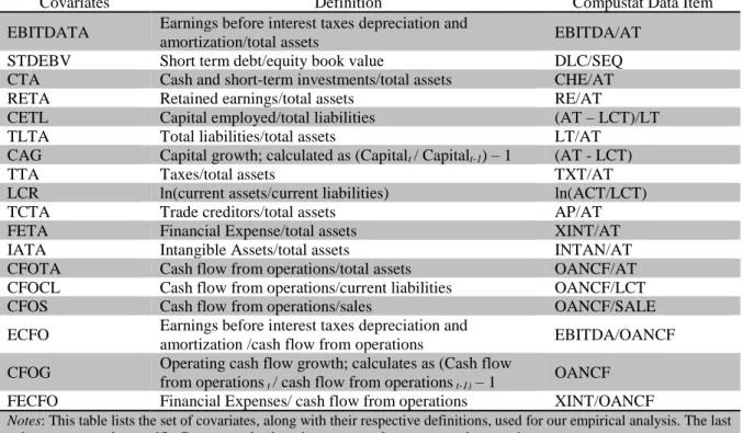
A large number of explanatory variables are discussed in the academic literature on firm default, financial distress and insolvency. We follow this literature in collating variables and conducting a number of first stage tests for their (joint) inclusion in the determination of financial distress or bankruptcy (see for example Altman and Sabato 2007, or Lin et al. 2012). This will be discussed further below, following a description of the explanatory variables and the reasons for their consideration in the modelling process. The variables included in the model are listed in Table 13.
Liquid assets might be drawn upon by a firm to meet immediate payments. Therefore, we expect that a firm with lower cash and short-term investments relative to total assets (CTA) will have a higher probability of default. A parallel argument might be made in relation to the scale of trade creditors to total assets (TCTA), with a larger value signifying greater immediate short-term claims on the firm and, therefore, a greater probability of default. Hudson (1986) reports that trade creditors are an important component of short term liabilities for many SMEs, and we might therefore expect this variable to have an effect on the probability of default. A further measure of the liquidity position of the firm is the log of current assets to current liabilities (LCR), where a higher value is expected to have a negative effect on the probability of default. A higher income tax paid in relation to total assets (TTA) is expected to have a negative effect on the probability of default, as firms having higher income are expected to pay higher taxes. The level of short term debt relative to equity book value (STDEBV) is also included as a measure proxying the short-term claims on the firm relative to capital employed. Short-term debt must be refinanced or repaid more immediately than is the case for other
3 While calculating respective financial ratios, we replace denominators having value 0 with small positive values
13 | P a g e sources of financing, and may be critical to the (involuntary) default of the firm if it is large. We take the capital employed divided by total liabilities (CETL) as an (inverse) measure of leverage. The larger the capital of the firm relative to the liabilities, the lower the expected default probability. Capital growth (CAG) is included as a higher rate of growth might indicate a growing capacity to meet financial obligations or to finance futures operations. This would suggest a lower probability of default. Total liabilities to total assets (TLTA) is also included as an explanatory variable, again as a measure of the financial fragility of the firm. Tangible assets are often found to be important in the determination of both capital structure and default.
Ceteris paribus a company with a higher level of tangible assets is more likely to obtain
external funding and to be offered re-financing in the event of difficulties. Further, Jones (2011) argues that firms in financial distress are more likely to capitalise intangible assets. We therefore include the ratio of intangible assets to total assets (IATA) as a predictor of default.
We employ a number of measures linked to earnings. The first of these is retained earnings relative to total assets (RETA). If a firm is nearing default, then we expect that this will be reflected in lower retained earnings. Conversely, even where the liquidity of the firm is under pressure, we would expect that a firm with relatively high retained earnings would find (re)financing easier and hence the probability of default lower. As we might expect earnings to be an important predictor of default, this is further explored through the inclusion of earnings before interest, tax, depreciation and amortization, again relative to total assets (EBITDATA). There is relatively little choice on the part of the firm in the determination of the value of this variable, the inclusion of which may therefore compliment the inclusion of RETA, where greater choice on the part of the firm’s managers may be evident. We also include financial ratios related to financial expense. Financial expenses relative to total assets (FETA) is included as a means to proxy the financial claims on the company, with a larger size of this variable expected to increase the probability of default. A similar argument holds for the financial expenses relative to cash flow from operations (FECFO).
An innovation in the analysis of default in US SMEs is the inclusion of variables related to cash flow from operations (henceforth CFO). We include a measure for cash-flow divided by total assets (CFOTA), with a high value suggesting a better asset utilization and hence lower default risk. Where current liabilities are used as the denominator, the resultant variable
14 | P a g e CFOCL is presented as a proxy for the ability of the firm to meet its obligations from CFO. With sales as the denominator we have the variable CFOS, a proxy for how effectively the firm manages its receipts/payments. We further include the growth in CFO (CFOG) as an indicator that the firm’s short term financial position and, hence, ability to meet its obligations will be improving with higher values of CFOG. The lower the rate at which earnings are translated to cash-flows, the worse, relatively speaking, the liquidity position of the firm. As we expect liquidity (rather than earnings) to influence default, we therefore anticipate that higher values of ECFO (earnings divided by operating cash-flows) lower the probability of default.
[Insert Table 1 Here]
3.3
Hazard Model
3.3.1 Basic Hazard Model
The analysis of default is derived from a survival function. Survival analysis addresses the time to the occurrence of an event, which in this study is the time until a default, being either a bankruptcy or financial distress. Suppose T is a non-negative random variable that denotes the time of a default event and t represents time itself. T then has a probability density function 𝑓(𝑡) or a cumulative distribution function (CDF) such that 𝐹(𝑡) = Pr(𝑇 ≤ 𝑡). A survival function, 𝑆(𝑡) is then given by the probability that 𝑇 > 𝑡, the reverse CDF of T.
𝑆(𝑡) = 1 − 𝐹(𝑡) = Pr(𝑇 > 𝑡)(1) At 𝑡 = 0, the survivor function is equal to one and moves toward zero as 𝑡 approaches infinity. The relationship between the survivor function and hazard function ℎ(𝑡) (also known as the conditional failure rate at the time𝑡) is mathematically defined as follows:
ℎ(𝑡) = lim ∆𝑡→0 Pr(𝑡 + ∆𝑡 > 𝑇 > 𝑡|𝑇 > 𝑡) ∆𝑡 = 𝑓(𝑡) 𝑆(𝑡) = −𝑑ln𝑆(𝑡) 𝑑𝑡 (2) The hazard rate is the (limiting) probability that the failure event occurs within a given time interval, given that the subject has survived to the start of the interval, divided by width of the interval. The hazard rate must be non-negative and varies from zero to infinity and may be increasing, decreasing, or constant over time. A hazard rate of zero signifies no risk of failure at that instant, while infinity signifies certainty of failure at that instant.
15 | P a g e
3.3.2 Discrete-Time Hazard Model
Some events may be experienced at any instant in continuous-time. This results in exact censoring and survival times, which will be recorded in relatively fine time scales such as seconds, hours or days. If there are no tied survival time periods, then under such circumstances a continuous-time survival model is an appropriate choice (Rabe-Hesketh and Skrondal 2012). However, in many cases the events are discrete or recorded at discrete intervals; for instance, expressing time to event in weeks, months or years. Where there are relatively few censoring or survival times with tied survival time periods, then a discrete-time survival model is more appropriate (again see Rabe-Hesketh and Skrondal 2012). Interval-censoring4 leads to discrete-time data, which is the case with our database. Here, the beginning and end of each discrete-time interval is the same for all of the SMEs, as the information is recorded on an annual basis. Thus, the event of interest may take place at any time within the year but it cannot be known until the information is provided at the end of the year. Hence, considering the discussion above, we estimate our hazard models in a discrete-time framework with random effects (𝛼𝑖), controlling
for unobserved heterogeneity or shared frailty.
The discrete-time representation of the continuous-time proportional hazard model with time-varying covariates leads to a generalized linear model with complementary log-log link (Grilli 2005, Jenkins 2005, Rabe-Hesketh and Skrondal 2012), specified as follows:
𝑐𝑙𝑜𝑔𝑙𝑜𝑔(ℎ𝑖(𝑡)) ≡ 𝑙𝑛{− 𝑙𝑛(1 − ℎ𝑖(𝑡))} = 𝛽𝑥(𝑡)𝑖′+ 𝜆𝑡(3)
Here, 𝜆𝑡 is time-specific constant which is estimated freely for each time period t, thus making no assumption about the baseline hazard function within the specified time interval. However, in most empirical studies logit link is used over complementary log-log (clog-log) link as specified in equation 4.
𝑃
𝑖,𝑡=
𝑒
𝛼(𝑡)+𝑥(𝑡)𝑖′𝛽
1 + 𝑒
𝛼(𝑡)+𝑥(𝑡)𝑖′𝛽(4)
4 The event is experienced in continuous-time but we only record the time interval within which the event takes
16 | P a g e Where 𝑃𝑖,𝑡 is the probability of experiencing the event by subject i at time t and α(t) captures the baseline hazard rate. This will produce very similar results as long as the time intervals are small (Rabe-Hesketh and Skrondal 2012) and the sample bad rate (% of default to non-default) is very low (Jenkins 2005). Thus, considering this discussion, we estimate our discrete hazard models using a logit link estimator.
3.3.3 Specifying Baseline Hazard rate
The baseline hazard rate is a necessary stage of analysis for the discrete hazard model. The specification of the baseline hazard function defines the probability of default given baseline values for the explanatory variables. Here we set all baseline values equal to zero. Time-varying variables are then identified that bear a functional relationship with survival times.
There are a number of alternate specifications for the baseline hazard function including log(survival time), polynomial in survival time, fully non-parametric, and piece-wise constant (see Jenkins 2005). For a fully non-parametric baseline hazard function, duration-interval-specific dummy variables need to be created (see Beck et al. 1998). However, this method becomes cumbersome if the maximum survival time in the dataset is very high, as in case of bankruptcy databases. A more parsimonious way of specifying the baseline hazard function is to use a piece-wise constant method. In this, the survival times are split into different time intervals that are assumed to exhibit a constant hazard rate (see Jenkins 2005). If there are time intervals (dummies) with no events, then the relevant observations from the estimation should be dropped as duration specific hazard rates cannot be estimated for them (Jenkins 2005, Rabe-Hesketh and Skrondal 2012). Considering the estimation convenience, the piece-wise constant specification of baseline hazard rate could be applied. However, if the hazard curve shows frequent and continuous steep rises and falls, then the piecewise approach may not be used and the fully non-parametric baseline hazard might be an appropriate choice.
3.4
Model Validation using ROC Curves
To evaluate the classification performance of the default prediction models developed, we present measures of their predictive accuracy. Out-of-sample validation regression models are first estimated up to 2010, with predictions made for bankruptcy and financial distress in
17 | P a g e 2011. The estimation period is then updated for a further year, ending in 2011, again with predictions made for the following year, with the updating process continuing until the final prediction year of 2014.
Model predictive performance is reported using Receiving Operator Characteristics (ROC) curves. These plot the true positives, where the model predicted a default which actually occurred, also known as sensitivity, on the ordinate axis. The false positives are plotted on the abscissa axis, where the firm defaults but the model failed to predict this, also known as fall out or (1-specificity). These are plotted because the discrimination threshold between defaulted and non-defaulted firms is varied. A 45o line would indicate no discriminatory power in the model; accordingly, deviations (above this) might be taken as an indication of predictive/discriminatory success. Therefore, the area under the ROC (AUROC) might be measured to provide a numerical value of model performance. Its value ranges from 0.5 to 1.0, which encapsulates the classification performance of the model developed. AUROC of 1 denotes a model with perfect prediction accuracy and 0.5 suggest no discrimination ability. In general there is no ‘golden rule’ regarding the value of AUROC, however anything between 0.7 and 0.8 is acceptable, while above 0.8 is considered to be excellent (Hosmer Jr et al. 2013).
4. Results and Discussion
To eliminate the influence of extreme outliers on our statistical estimates, we restrict the range of all our financial ratios between the 5th and 95th percentiles. In addition, we lag all our variables by one-year to ensure that all information employed in prediction is available at the beginning of each year. Note that default is recorded during the year in which it takes place to ensure that fitted values for the dependent are not based on financial information presented in the same year, as some information would post date the default event.
4.1
Failure Rate and Descriptive Statistics
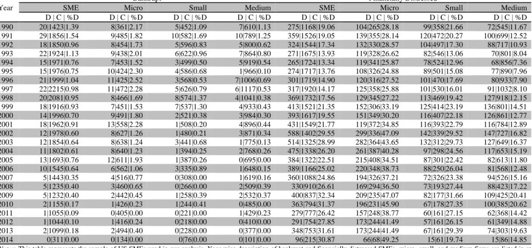
Information on the sample for the dependent variables is presented in Table 2, disaggregated by SMEs size classification and failure type (bankrupt and financially distressed firms).
18 | P a g e Notwithstanding the number of SMEs filing for bankruptcy is small in absolute terms, bankruptcy aggregated data delineates an apparent decline in incidence over the time window analysed (especially after around 2001). Data seems to suggest different trends when bankruptcy is disaggregated by SMEs size categories. Indeed, the ‘micro firm’ set represents the largest single component of the total (with only a few exceptions). In particular, this tendency is confirmed in this century. The same might also be said for firms that are financially distressed. Indeed, micro firms are always the largest group of financially distressed firms and their relative importance is growing over time, especially during this century (in line with the bankruptcy trend). Distress rates for this group have been above 40% for much of the time since the dotcom bubble in 2002. Although cohort sizes may vary, these simple descriptive statistics reinforce the interest in examining the determinants of default events separately. This evidence provides strong support for our hypothesis H1. Default numbers and proportions do not appear to be consistent across the different size classifications of SMEs, whether firms are filing for legal bankruptcy or entering financial distress. Note might also be taken of the very large number of firms that are facing financial distress, and the challenges and importance of predicting distress for external providers of capital. Further details on sample description and descriptive statistics for the explanatory variables can be found in Appendix A5.
[Insert Table 2 Here]
4.2
Analysis of Survival and Hazard Curves
As discussed earlier, it appears that the likelihood of default changes over time and, consequently, a simple statistical test (such as a t test) may be misleading. In the context of survival analysis, many of the alternative measures were specifically developed for continuous-time models and may also suffer from bias when applied in a discrete-continuous-time framework. Consequently, we estimate univariate hazard models and report average marginal effects (AME) for each variable to facilitate the specification of the later multivariate model. The usual marginal effects report on the change in the conditional mean default in the baseline model as a consequence of a marginal change in one of the explanatory variables6. However, this paper
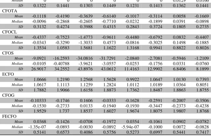
5 Table A1 reports descriptive statistics outlining any potential discriminatory power of a set of explanatory
variables, according to their type of failure (bankruptcy vs financial distress).
19 | P a g e first estimates a marginal effect for each observation and, then, the average across the marginal effects to obtain AME. The absolute values of the AME are ranked, as a guide to later model specification, and their statistical significance is reported. In case the variables for the SME category are statistically significant, we reported the p-value for a Wald test of the equivalence of the estimated coefficient for each of the size categories. The rationale behind this analysis is two-fold: first, it provides early evidence of whether the determinants of default are similar across different categories of SMEs; and second, it informs the proceeding model specification.
Figure 1 presents survival and hazard curves for our sample of micro, small and medium firms. These show the hazard of bankruptcy and financial distress for the different size classes of SMEs. Reflecting on the discussion of the previous section, the hazard rates for bankruptcy are lower than for financial distress; conversely, the survival rates are higher for bankrupt firms in comparison to firms experiencing financial distress. This reinforces our argument that, at a given age, the likelihood of financial distress is much higher and significantly different from bankruptcy likelihood. The top part of Figure 1 presents survival curves for the bankrupt and distressed groups of firms for different SMEs size categories. From these graphs, it emerges clearly that survival rates with respect to firms’ age vary with firms’ size. Larger firms tend to have better survival rates than smaller firms. In particular, for the bankrupt group of firms, the survival rate of micro firms is significantly lower (conversely hazard curves are significantly higher) than small and medium-sized firms. Although the survival curve of small firms is lower than that of medium firms, they are very close to each other throughout. This suggests that both small and medium-sized firms exhibit quite similar bankruptcy attributes. However, for financially distressed firms all three size groups exhibit sufficiently different survival rates. Also, as might be expected from the preceding statistics, a higher hazard rate is found for financially distressed firms in Figure 1 than for their bankrupt counterparts, although the patterns differ. In line with the previous results, micro firms are most vulnerable to financial distress, followed by small and medium firms respectively. For micro firms, the hazard rate for financial distress rises but then falls from around 30 years. By contrast, the hazard rate for small firms shows a rise until an age of around 20, then plateaus before rising steeply again. The pattern to the hazard rate for financial distress for medium firms reports general moderate rise. These differences in hazard rates across size categories of bankrupt and financially distressed firms reinforces our hypothesis (H1) that default attributes of SMEs vary with firms’ size.
20 | P a g e Further, the hazard curves do not follow any consistent parametric shape. Thus, a fully non-parametric baseline hazard specification seems to be an appropriate choice. In light of this discussion, in the following section, we employ firm age specific dummy variables in our multivariate models to proxy the baseline hazard rate.
[Insert Figure 1 Here]
4.3
Univariate Hazard Analysis
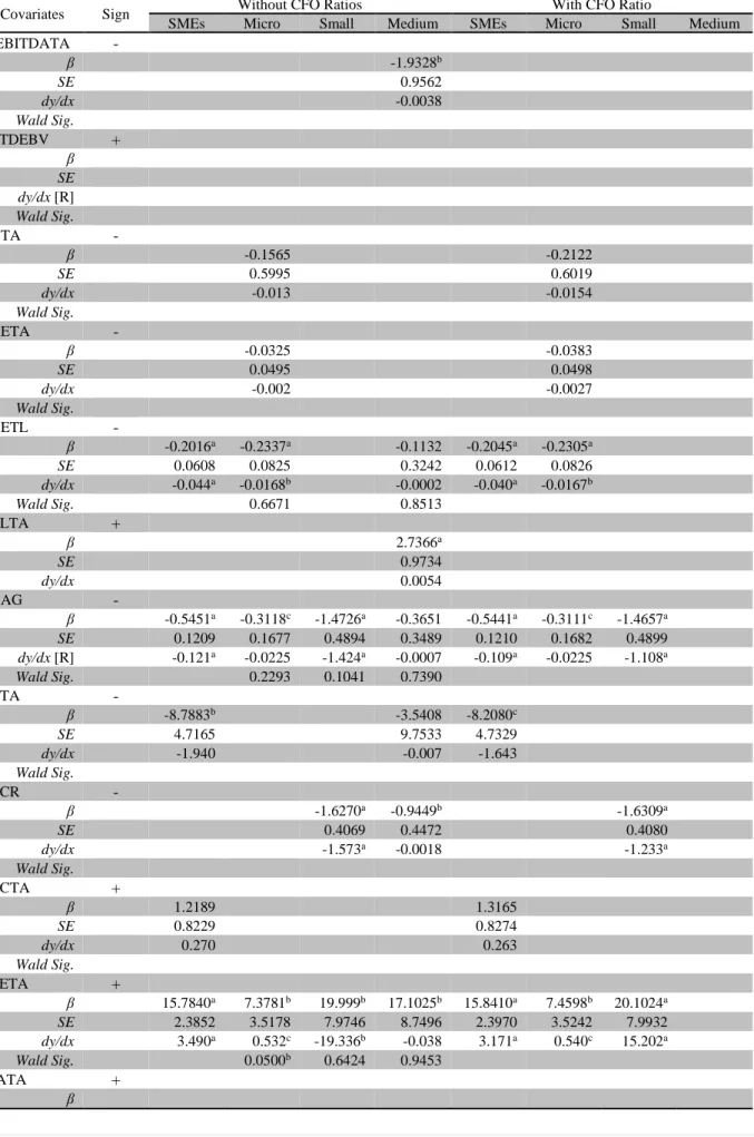
The results of univariate modelling are presented in Table 3, with columns reporting on findings for SMEs as a whole and for each SMEs size sub-categories, disaggregated by bankrupt and financially distressed firms respectively. For each variable, the first row shows the coefficient estimates, together with an indication of statistical significance. The second row indicates the standard error. The AME are presented in the third row with their ranking (for the column concerned). Appropriate Wald statistics are then presented in the final row.
4.3.1 Non-Cash Flow Covariates
Section A of Table 3 reports the results for non-cash flow covariates. Earnings (EBITDATA) demonstrate discriminatory power over the baseline model for both bankrupt and financially distressed firms, with the exception of micro and small firms in the bankrupt part. All cases in which this variable presents a statistically significant coefficient, it has also a rank for the AME of 6 or better. In the case of bankrupt firms, the effect appears to be driven by the medium category, and this result informs the further model specification. In the case of short term debt (STDEBV) only the medium category of financially distressed firms indicates discriminatory power over the baseline model, though with the expected positive sign for the estimated coefficient. The estimated coefficients for the variable cash scaled to total assets (CTA) have the expected negative signs and are all statistically significant. Ranks for the AME are high, but multicollinearity issues restrict the use of this variable in the full model when considering bankrupt firms. Retained earnings (RETA) also have the expected negative and statistically significant signs in univariate estimation but have low rank for the AME, with the possible exception of bankrupt micro firms. Similarly, capital employed (CETL) has the expected negative and statistically significant effect across the board. However, the rank of the AME is low for financially distressed firms; this is reflected in the multivariate model
21 | P a g e specification. Liabilities relative to total assets (TLTA) have a strong effect in a univariate setting but the variable is correlated with other variables in the full model, where its use is somewhat restricted. In considering the results on capital growth (CAG), which is a variable included in most of the multivariate models, the estimated coefficients confirm the expected sign. The rank for the AME, especially in the case of bankrupt firms, is high. The Wald statistics suggest a different response by size classification. In an examination of the effect of taxes (TTA), there are two cases where the estimated coefficients are of an unexpected sign (micro in bankrupt firms) or are statistically insignificant (small in bankrupt firms). However, in the other univariate results for this variable, the expected positive effect also has a highly ranked discriminatory power, commending its inclusion in the multivariate setting. The ratio of current assets to liabilities (LCR) ranks most highly for small bankrupt firms, when examining the AME, with the lowest rank being for medium-sized financially distressed firms. Trade creditors (TCTA) are also found to have significant discriminatory power against the baseline model, and the variable ranks highly on the basis of AME. However, the Wald statistics do not suggest that the effects differ greatly across different categories of bankrupt firms. Greater levels of financial expense (FETA) have the expected positive effect on default probability (relative to the estimated baseline). The variable also ranks highest on the basis of AME for all but one case, and the response appears to be different across size categories. The variable measuring intangible assets (IATA) has no discernible discriminatory power above the baseline model for bankrupt firms and the AME are ranked low where this is the case of financially distressed firms.
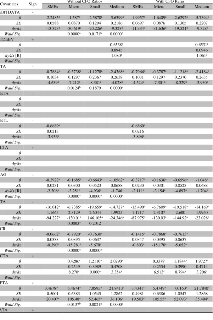
4.3.2 Cash flow Covariates
The remaining sub-set of variables reference operating cash-flows and the results for the univariate hazard analyses on these variables may be found in Section B of Table 3. A relatively large number of estimated coefficients presents either an unexpected sign and/or is statistically insignificant in estimation. For bankrupt firms, operational cash-flows divided by assets (CFOTA), liabilities or sales have little discriminatory power relative to the baseline model. However, earnings divided by cash-flow (ECFO) provides some evidence of effect for bankrupt firms. Cash-flow growth and financial expenses divided by cash-flow (CFOG and FECFO) respectively provide little evidence of discriminatory power over the baseline hazard
22 | P a g e model, however. This result is consistent with the findings of similar studies, such as Mazouz
et al. (2012) and Gupta et al. (2014).
Cash-flow variables demonstrate some further discriminatory power over the baseline model in predicting financial distress. For the variable cash-flow divided by total assets (CFOTA) all coefficients are of the expected sign and statistically significant. The AME are also significant, however the correlation coefficients were rather high (especially with earnings variables). For this reason, this variable was not included in the multivariate models. The level of operating cash-flow divided by current liabilities (CFOCL) is of the expected sign and is statistically significant both overall and for most classes of financially distressed firms. This merits inclusion of the variable in the later analysis, again in conjunction with a consideration of any multicollinearity. Where cash-flow is divided by sales (CFOS) the evidence is mixed with statistical significance of a coefficient only found in the case of medium sized firms and an insignificant Wald statistic. The results are similar where earnings are divided by cash-flow from operations (ECFO). However, cash-flow growth (CFOG) provides a more interesting case. For all cases of financially distressed firms, the estimated coefficients are of the expected sign and are statistically significant. The AME are also significant and there is evidence that the effect is different for different size classes of firm. The results for financial expenses (FECFO) are counter intuitive and, unlike the CFOG variable, are therefore excluded from the multivariate models.
In line with our observation in Figure 1, an identical set of covariates is significant in explaining bankruptcy and financial distress for different SMEs size groups in the majority of the cases. However, overall, the coefficients of covariates for micro firms are significantly different from SMEs, both in the case of the bankrupt group of firms and in those financially distressed. This also holds true for a few covariates within the small and medium size groups (e.g. CTA, TLTA, FETA, LRC). As reported in Table 3, the magnitude of coefficients of a given covariate also varies significantly across micro, small and medium firms for both bankrupt and financially distressed sample groups.
These results provide preliminary support for our hypotheses H2, H3 and H4. [Insert Table 3 Here]
23 | P a g e
4.4
Multivariate Discrete Hazard Models
In this section, we estimate multivariate discrete-time duration-dependent hazard models with logit link across size categories (respectively for SMEs, micro, small and medium firms) for bankruptcy and financial distress respectively. The dependent variable has a binary outcome with financially distressed/bankrupt equal to ‘1’ and ‘0’ otherwise, while independent variables are the set of covariates found to be significant in the univariate regression analysis. Considering the multicollinearity among the covariates, we introduce each significant covariate in turn into the multivariate setup based on the magnitude (sign is ignored) of their AME. For this, we first rank7 all the covariates found to be significant (with the expected sign) in the univariate analysis, based on the absolute value of their AME. Following Gupta et al. (2018), we then introduce each covariate in turn into the multivariate model in increasing order of the rank of their AME, the rationale being the higher the value of AME, the higher the change in the predicted probability due to a unit change in the covariate. Thus, a covariate with a higher value of AME (e.g. FETA) is more efficient in discriminating between distressed and censored firms than covariates with lower values of AME (e.g. TLTA). Further, if the introduction of a covariate flips the sign of any previously added covariate, then that covariate is excluded from the multivariate model. This situation can possibly occur due to multicollinearity among covariates; accordingly, excluding these covariates seems to be a reasonable choice. We believe that this method of covariate introduction, while developing the multivariate models, leaves us with the best set of covariates with the expected sign of respective coefficients. Initially the multivariate models are estimated using financial ratios obtained from the income statement and balance sheet only, as, amongst others, we examine the information content of cash-flow information. Subsequently, we estimate an additional set of models supplemented with significant operating cash flow ratios. We also control for a volatile macroeconomic environment affecting specific industrial sectors. For this, we calculate an additional measure of industry risk (Risk) separately for SMEs, micro, small, and medium firms as the failure (bankrupt/financial distress) rate (number of firms experiencing the event of interest in respective industrial sectors and respective size categories in a given year/total number of firms in that industrial sector and size category in that year) in each of the seven industrial sectors in
7 However, cash-flow ratios are not included in the ranking process to assess their incremental information content
24 | P a g e a given year8. Higher values indicate a higher failure risk, and vice versa. To assess the
classification and validation performance of the models developed, area under ROC curves are also estimated (further details of these analyses can be found in Graph A1 and Graph A2 in the Appendix).
4.4.1 Multivariate Hazard Models for Bankrupt Firms
SMEs: We start with a report on the multivariate hazard model for bankrupt SMEs without cash-flow variables in the first column of Table 4. The last rows of this column report on the goodness of fit measures. The Wald Chi Squared measure indicates that the included variables are jointly statistically significant at a 99% level. Both within sample and out-of-sample AUROC statistics confirm that the model performs well, with both values over 70%.
Capital employed divided by total liabilities (CETL) and capital growth (CAG) show the expected negative sign, which is statistically significant at the 99% level. Their AMEs are also statistically significant. Accordingly, firms are less likely to file for bankruptcy when in the presence of higher levels of capital. Similarly, firms with stronger capital growth are also less likely to file for bankruptcy. Taxes (TTA) also have the expected negative effect on the probability of bankruptcy. Although the estimated coefficient is statistically significant at a 95% level, this cannot be said for the AME. Thus, the conclusion on the effect of taxes is mixed, certainly in terms of economic significance. Trade creditors (TCTA) do not have an effect on the basis of the results presented for SMEs, however financial expenses (FETA) do. Both the estimated coefficient and the AME have a statistically significant effect at a 99% level in their positive effect on the probability of bankruptcy. The accuracy of results as well as the signs and significance of few variables for SMEs are compatible with the results of similar studies such as Altman and Sabato (2007) and Altman et al. (2010). However, as shown in the next sections, the impact of the variables and their significance vary when we divide SMEs into respective size categories.
The addition of a cash-flow variable, namely earnings divided by cash-flow (ECFO)9, does bring further predictive power. This is not to the extent that there are any changes in the
8 Further information on the industrial classification can be found in the Appendix (Table A2). 9 The Wald test confirms the joint significance of the variables and the AUROC results are equivalent.
25 | P a g e interpretation of the variables from the first model. The estimated coefficient for ECFO is negative as expected and the result statistically significant at a 99% level. This provides further support for concluding that earnings mediated by cash-flow is a significant influence on the probability of bankruptcy, as the AME is also statistically significant (though only at a 90% confidence level).
Micro Firms: In the case of the micro category of firms, the previous univariate analysis
and the review of the correlation matrix recommended i) the exclusion of taxes (TTA) and trade creditors over total assets (TCTA); and ii) the inclusion of two further variables (namely, short term cash and investments (CTA) and retained earnings (RTA). Both CTA and RETA are not statistically significant for estimation in the multivariate model without the cash-flow variables. Compared to the SMEs category, capital employed (CETL) retains the expected sign and significance for both the coefficient and AME. The result of a Wald test of the equivalence of the coefficients from the micro firms shows that there is no significant difference between the two coefficients. The coefficient on capital growth (CAG) is negative and statistically significant, as in the SME case. Conversely, the result for AME - even with the same sign - loses its statistical significance. The Wald test finds no difference between the value for this coefficient and the one for the SMEs as a whole. The result related to financial expenses (FETA) seems to uncover a different role played by this covariate in predicting bankruptcy. As in the SME case, FETA is found to be statistically significant both in estimation and in the average marginal effect. However, this ratio of financial expenses to cash-flow has an estimated coefficient that is half the size of that for SMEs as a whole, and the AME is much lower for micro firms. This is confirmed by the Wald test for the equality of coefficients, leading to the conclusion that the FETA is significant in predicting bankruptcy but the size of effect is lower.
The results described in this section are not entirely consistent with the relevant studies, such as Gupta et al. (2015). This study finds CTA and RETA, two significant indicators of micro firms’ financial failure. However, they suggest that micro firms should be considered separately in the process of failure prediction, which is in line with our findings. The inclusion of the previous cash-flow variable (ECFO) does not add to the explanatory power of the model. This result seems to be in contrast to the model for SMEs as a whole.
26 | P a g e
Small Firms: The third results column for Table 4 references the estimates predicting
bankruptcy for small firms, in a model excluding the cash-flow variables. Goodness of fit measures indicate that the included variables are jointly significant and there is a reasonably high predictive power both within and outside sample. Three variables were included based on the univariate analysis: i) capital growth (CAG) and financial expenses (FETA) as in the SMEs model; and ii) ratio of current assets to liabilities (LCR), which has not been considered before. CAG has the expected negative sign for the coefficient and is statistically significant at a 99% level. In scale, the estimated coefficient is larger in absolute terms than that for SMEs as a whole; however, the Wald test does not indicate that there is a significant difference. LCR has the expected negative sign, is statistically significant at a 99% level, and has a significant average marginal effect. FETA appears consistently through our modelling of bankruptcy prediction and has the expected positive sign here with a statistically significant estimated coefficient and AME. However, in contrast to the finding for micro firms, the Wald test for the equality of coefficients does not suggest that there is a difference between small firms and SMEs as a whole.
The addition of the cash-flow variable earnings divided by cash-flow (ECFO) does not add to the explanatory/predictive power of the model in this case, leaving the findings for the first model, immediately above, to stand.
Medium Firms: The model specification10 for medium firms differs slightly from the
univariate analysis. An examination of the correlation coefficients for this sample i) admitted earnings (EBITDATA), liabilities divided by assets (TLTA) and the (log of) current assets divided by current liabilities (LCR) to the model; and ii) excluded the trade creditors over total assets (TCTA). The coefficient on EBITDATA carries the expected negative sign and is statistically significant at a 95% level, although the AME is not statistically significant. Capital employed divided by total liabilities (CETL) is statistically insignificant in estimation. This result seems to be inconsistent with the results of Gupta et al. (2015). However, total liabilities divided by total assets (TLTA) has the expected positive coefficient in estimation and is statistically significant at a 95% level. The AME is not statistically significant, suggesting that
10 The included variables are jointly significant at a 95% level and the model has the highest in sample AUROC
27 | P a g e the finding is not robust across all observations. Capital growth (CAG) was found to have a significant effect on the probability of default in all previous models; conversely, it is not the case for the medium-sized firm category. Taxes (TTA) do not have an effect, although the coefficient is of the expected sign. The (log of) current assets divided by current liabilities (LCR) does have the expected sign for the estimated coefficient, but the AME is not significant. As noted earlier, financial expenses relative to assets (FETA) is of the expected positive sign and also statistically significant. As the coefficient estimate is similar in size to that for SMEs as a whole it is perhaps unsurprising that the Wald test fails to reject the null of equivalence (although of course note should be taken that the test is of a different nature).
No cash-flow variables were suggested as an addition to the above and so no further model results are presented for the medium firms’ category.
In summary, from this analysis, we can conclude that factors affecting the bankruptcy of SMEs do vary across size categories. Amongst others, we highlighted the different role play by FETA in predicting bankruptcy of micro-sized firms compared to the SMEs category. Furthermore, in contrast with Gentry et al. (1987) and Gilbert et al. (1990), CFO information does not provide any marginal improvement in models’ classification performance above information obtained from income statements and balance sheets. These results for micro, small and medium SMEs strongly support our two hypotheses H2 and H3. At the same time, they are not entirely consistent with Gupta et al. (2015), who conclude that there is no need to consider small and medium categorised firms separately in modelling their credit risk. Finally, the analysis leads us to accept H4 only in the univariate dimension, as operating cash flow information does not add any marginal increment in prediction performance of hazard models above income statement and balance sheet in the multivariate framework. Our results corroborate the empirical evidence provided by Gupta et al. (2015) for our sample of UK SMEs.
[Insert Table 4 Here]
4.4.2 Multivariate Hazard Model for Financially Distressed Firms
Firms that have declared bankruptcy have, arguably, experienced greater problems than those that are in some form of financial distress. However, as discussed earlier and following