Wavelet discrete transform, ANFIS and linear regression for
short-term time series prediction of air temperature
Devi Munandar
Research Center for Informatics- Indonesian Institute of Sciences, Gedung 20 Lt 3, Jl.Cisitu (Komplek LIPI) No.21/154D, , Bandung, Indonesia
I. Introduction
An air temperature conditions from year to year changes along with the global warming is happening in the world. Cyclical changes in cropping patterns by farmers of maize, rice, vegetables, wheat and others have traditionally been a shift in the stage of planting to harvest. The condition of the river is always in the flow of water will turn to the adequacy of the consumption of agricultural land as well as the flora and fauna that needed water. The rising temperature changes resulting forest fires and pollution on living beings. It needs the knowledge to predict the temperature to do preventive actions considered to overcome the undesirable condition and as a reference for mitigation.
In reality, air temperature prediction was done for research purposes for modeling such as; climate change, ecology, hydrology, the work was done to determine changes in the atmospheric environment [1]. Many models have been developed to predict the temperature like statistical models and numerical computing.
Research on the temperature change that affects the cycle of hydrological was conducted in Europe. It performs the change-point detection techniques for identification of affected temperatures climate changes affect the temperature. Researchers modeled annual temperature changes based on TMin and TMax by using Bayesian and Linear Regression [1]–[3].
On the other hand, research of hybrid wavelet and Support Vector Machine (SVM) was conducted to forecast monthly river flow. As a result, the hybrid model error is smaller than the original SVM [4]. Wavelet transform is also in use for clustering the spatial-temporal Taiwan rainfall data within 22 years [5]. The wavelet transformation is also effective for short-term electrical power forecasting [6]. Furthermore, it shows that the wavelet methods can be implemented as an encouraging and effective methodology to predict potential of a wind power plant [7], [8]. Fuzzy Sugeno Mamdani is part of alternative artificial intelligence method, can be used for rainfall and weather prediction [9], [10].
This research tries to investigate representation of discrete wavelet transform and Adaptive Neuro Fuzzy Inference System (ANFIS) in weather parameters modeling. Linear Regression is used as the baseline of the developed prediction model.
ARTICLE INFO A B S T R A C T
Article history:
Received August 8, 2017 Revised August 18, 2017 Accepted August 18, 2017
This paper investigates the ability of Discrete Wavelet Transform and Adaptive Network-Based Fuzzy Inference System in time-series data modeling of weather parameters. Plotting predicted data results on Linear Regression is used as the baseline of the statistical model. Data were tested in every 10 minutes interval on weather station of Bungus port in Padang, Indonesia. Mean absolute errors (MAE), the coefficient of determination (R2), Pearson correlation coefficient (r) and root mean squared error (RMSE) are used as performance indicators. The result of Plotting ANFIS data against linear regression using 1-input data is the optimal values combination of output predictions.
Copyright © 2017 International Journal of Advances in Intelligent Informatics. All rights reserved.
Keywords:
Discrete Wavelet Transform Linear Regression ANFIS
Sub-Time Series Data Plotting data
II. Methodology and Concept A. Object Study Location
The studied region is the monitoring station at Bungus fishery port in Padang, Indonesia (Fig. 1). The stations were built by the Research Center for Informatics - LIPI in cooperation with the Research Station Resources and Coastal Vulnerability (LPSDKP) of Ministry of Maritime and Fisheries Affairs. Monitoring station in Bungus port located on the west coast of Sumatera Island (1.0301107 latitudes and 100.395639 longitudes). Bungus Ocean Fishery Port frequented by many fishing vessels above 60 GT. These boats are generally types of long liner and purse-seiner the fishing ground in deep water or until ZEEI Indian Ocean. Nearly twice weekly tuna boats unload their catches in this port and hereinafter will be exported to Japan and America.
The second location named weather monitoring station Muaro-Anai, close at Minangkabau International Airport. Measured data from Bungus monitoring stations is then stored to the LIPI server in every 10 minutes. Observed temperature data April to July 2016 is characterized as the short-term prediction with 8335 data pairs1.
Fig. 1. Weather monitoring station and tide gauge station at Bungus port, Padang city, West Sumatera Province - Indonesia
In conducting the prediction data set is divided into training data (6668 10 minutes interval data, 80%) and testing data (1667 data 10 minutes interval, 20%). As in Table.1 every 10 minutes interval data statistically with variable sets TMean, TMedian, TMode, TMax, TMin, TStdev, TRange. Generally, each
variable represents the Mean, Median, Minimum, Maximum, Standard Deviation and Range of temperature measurement results at the Bungus weather station. Tmin, Tmax representing Temperatures between 21.76 until 34.71 oC for training data sets, 21.47 to 33.16 °C for testing data sets, and 21.47
to 34.71°C for the entire data sets. Distribution of data can be observed from weather measurements Bungus station looks distribution of data almost evenly in both the training data, the testing data or entire data autocorrelations high enough, showing consistency tends to be high and evenly (for example, r1 = 0993, r2 = 0981, r3 = 0967, r4 = 0950) has high distribution of data.
Table 1. Variable input data statistically Data set (T oC) Training Data Testing Data Entire Data TMean 27.53 26.46 27.31 TMedian 26.89 25.46 26.75 TMode 25.86 24.00 26.10 TMax 34.71 33.16 34.71 TMin 21.76 21.47 21.47 TStdev 2.55 3.11 2.70 TRange 12.95 11.69 13.24 r1 0.992 0.992 0.993 r2 0.980 0.980 0.981 r3 0.966 0.964 0.967 r4 0.949 0.947 0.950
B. Mackey Glass Chaotic Time Series
The Mackey glass equation is nonlinear time delay differential equation [8]:
𝑑𝑥 𝑑𝑡 = 𝛽
𝑥(𝑡−𝜏)
1+(𝑥(𝑡−𝜏))𝑛− 𝛾𝑥(𝑡)
For𝛽, 𝛾, 𝑛 > 0
(1) τ is a nonnegative delay time for evaluating the signal. n is a non-negative parameter that helps to illustrate the feedback/response time-delayed. β and γ are two nonnegative parameters in the equation (1). Since this is delay differential equation, initial conditions must be determined at the interval, and that made it infinite dimensional systems.
C. Discrete Wavelet Transform
Discrete Wavelet Transform (DWT) is data frequency decomposition. Implementation of discrete wavelet transformation can be done by passing the signal through a low pass filter (low pass filter / LPF) and high passes filter (high pass filter / HPF) and perform down sampling on the output of each filter. The wavelet transform is scientific tools for nonlinear and non-stationary of signal analysis [7]. To overcome this difficulty, DWT has two scales of transformation algorithms, can be implemented in applied approach. In this case, it can reduce the computational complexity of other wavelet models such as the Continuous wavelet transform (CWT) [10].
𝑊𝑎,𝑏= 2−𝑎/2∑𝑁−1𝑡=0 𝜓(2−𝑎𝑡− 𝑏)𝑥𝑡 (2)
Where t is an integer data type for the time, a and b is also a controller, each of scale and timing;
Wa,b is the wavelet coefficients for the scale factor, s =2 a is the time factor, and τ = 2ab. On the
Discrete Wavelet Transform method, time-series data pass through two kinds of filter and wavelet decomposed into components of sub-time series, which were computed from the equation (2), without losing the element of instant information. Discrete Wavelet Transform conducted transformation the signal to a father and mother wavelet. Father wavelet represent the high-scale, low-frequency components (approach (A) component). Mother wavelet is a representation of scale low and high-frequency components (detail (D) component). To do decomposing signal x(t) into a detail of the hierarchical structure (high frequency) and approximations (low frequency) to some degree levels as follows:
𝑥(𝑡) = 𝐷1+ 𝐷2+ 𝐷3+ ⋯ + 𝐷𝑛+𝐴𝑛 (3)
In the equation (3), D1, D2, D3,… , Dn show detail coefficients, and An show the approximation of nth
level.
D. Adaptive Neuro Fuzzy Inference System (ANFIS)
Before recognizing ANFIS, using ANN becomes a good reference used in modeling [11]. Neuro fuzzy is selected to manage linguistic factors, in this case for weather prediction. It is good for quality modeling human knowledge base and Alternative for decision making. Artificial Neural Network has potential learning. ANN can recognize patterns, just as humans do, which can be input and generate predictions. Integrating ANN and fuzzy logic can further improve performance, minimize errors and flexibility. In Fig. 2, ANFIS model for two inputs, in this figure seen circle and box are symbolizes non-adaptive and adaptive variable [12]
Takagi-Sugeno model is a much more effective option to use especially at the time of calculation and more adaptive [9].
The ANFIS with two inputs the rules as following:
𝐑𝐮𝐥𝐞𝟏: 𝐢𝐟 (𝒙 𝐢𝐬 𝑨𝟏) 𝐚𝐧𝐝 (𝒚 𝐢𝐬 𝑩𝟏), 𝐭𝐡𝐞𝐧 𝒇𝟏= 𝒑𝟏𝒙 + 𝒒𝟏𝒚 + 𝒓𝟏 (4)
𝐑𝐮𝐥𝐞𝟐: 𝐢𝐟 (𝒙 𝐢𝐬 𝑨𝟐) 𝐚𝐧𝐝 (𝒚 𝐢𝐬 𝑩𝟐), 𝐭𝐡𝐞𝐧 𝒇𝟐= 𝒑𝟐𝒙 + 𝒒𝟐𝒚 + 𝒓𝟐 (5)
Fig. 2. ANFIS model for two inputs [9]
Layer1: In this layer the connected inputs are adaptive can be changed as follows:
𝑂1,𝑖= 𝜇𝐴𝑖(𝑥)For i=1, 2 or (6) 𝑂1,𝑖= 𝜇𝐵𝑖−2(𝑦)For i=3, 4 (7)
In equation (6) (7) can be seen x and y are input node i, 𝐴𝑖 and 𝐵𝑖 are linguistic label labels
connected with node. 𝜇𝐴𝑖 And 𝜇𝐵𝑖 is the membership function of each node.
Layer2: In this layer a circle node labeled Π is non-adaptive symbol. This function can be used also if the part of the premise is consistent and has some fuzzy set. This condition using multiplication operators:
𝑂2,𝑖= 𝑤𝑖=𝜇𝐴𝑖(𝑥). 𝜇𝐵𝑖(𝑦)For i=1, 2 (8) Layer3: In this layer, label N in the middle of circle use to normalize with calculate ratio of node i and sum of firing strength, the node function:
𝑂3,𝑖 = 𝑤̅𝑖= 𝑤1 𝑤1+𝑤2= 𝑤𝑖 ∑ 𝑤𝑖, For i=1, 2 (9)
Layer4: In this layer output from equation (9) (layer 3) is multiplied with equation (4) and equation (5) as following function:
𝑂4,𝑖= 𝑤̅𝑖. 𝑓𝑖= 𝑤̅𝑖(𝑝𝑖𝑥 + 𝑞𝑖𝑦 + 𝑟𝑖)For i=1, 2 (10) Layer5: In this layer all parameters corresponding to the mechanism are added to be output. This layer is fixed.
𝑂5,𝑖 = ∑ 𝑤𝑖̅𝑖. 𝑓𝑖= ∑ 𝑤𝑖 𝑖.𝑓𝑖
∑ 𝑤𝑖 𝑖 (11) E. Linear Regression
Linear Regression is corresponding to create between variables with rule dependencies. There are 2 types of variables that are defined: independent variables and dependent variables. Variable Z
shows the result of the estimated calculation in equation (12). This process is show dependent variable, while the independent variable is X. both of these variables has interconnection. If an equation there is one variable X then this is called simple regression, while the independent variable is more than one, it is called multi linear regression. The function as following:
𝑍 = 𝛫0+ 𝛫1𝑋1+ 𝛫2𝑋2+ ⋯ + 𝛫𝑛𝑋𝑛For i=1, 2…n (12) Z represent dependent variable, 𝛫0− 𝛫𝑛 parameters that need in equation, while 𝑋1− 𝑋𝑛 is
F. Performance of Evaluation Criteria
Frequently measure used to analyze Wavelet model as following:
𝑀𝐴𝐸 = 1 𝑛 ∑ |𝑂𝑖− 𝐸𝑖| 𝑛 𝑖=1 (13) 𝑅2= [∑ (𝑂𝑖−𝑂)(𝐸𝑖−𝐸) 𝑛 𝑖=1 ]2 ∑𝑛𝑖=1(𝑂𝑖−𝑂) ∑𝑛𝑖=1(𝐸𝑖−𝐸) (14) 𝑅𝑀𝑆𝐸 = √∑𝑛𝑖=1(𝐸𝑖−𝑂𝑖)2 𝑛 (15) 𝑟 = ∑𝑛𝑖=1(𝑄𝑖−𝑄)(𝑆𝑖−𝑆) √∑𝑛𝑖=1(𝑄𝑖−𝑄)2 √∑𝑛𝑖=1(𝑆𝑖−𝑆)2 (16)
n is numbers of set data test, while the Linear Regression, ANFIS and Wavelet model are shown by Qi, Oi as observation value and Si, Ei represent estimation value. 𝑂, 𝑄 is average value of observation and 𝐸, 𝑆 is the average value estimates.
III. Results and Discussion
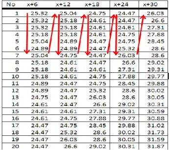
At the initial stage, data’s are separated into training and testing data using equation (1). To utilize the data in present with the time series required collection of data within a certain time. For example, when t is the reference value for predicting the next minutes, then the value is t + P. The standard method for this kind of forecast to create a mapping from D point data sample, a sample of each unit Δ in time, (x (t (D-1) Δ), ..., x (t-Δ), x (t)), with a predicted next value x (t + P). After an ordinary arrangement for predicting Mackey Glass time series data, set D = 4 and Δ = P = 6. For each t, the training data input for Wavelet and Linear Regression is a four-dimensional vector of the shape of each sub-time series as following
w (t) = [x(t+6) x(t+12) x(t+18) x(t+24)] as an input and s(t) = x(t+30) as an output with the distribution of the output values data are separated into training and testing data, x(0) = 1.2, τ = 27, and x(t) = 0 for t <0.
All of 8335 data pairs used to facilitate the 8200 data pairs. Initialize the data, start 28th to 8227th
with the initialization of data to be divided into five intervals of data. Fig. 3 show the data will be started of the interval x + 6. In other words, for 10 minutes interval x + 6 = 60 minutes, x + 12 = 120 minutes, x + 18 = 180 minutes, x + 24 = 240 minutes.
Fig. 3. Mackey Glass time series temperature data model A. Wavelet and Linear Regression Models
Temperature data is used, like time series format in decomposing into various sub time series components (DS) using the Discrete Wavelet Transform (DWT) to estimate the temperature next t
minutes. Five levels of resolution wavelet were used in this study. Stages (n = 1, 2, 3, 4, 5) while branching decompose resulting from the process is 2n (2-4-8-16-32). Qt refers to D as sub-time series at time t+i and temperature measurements at time t. All data time-series with 10 minutes interval is used in this model. Relationship values information for resolve of valuable components of wavelet on the temperature. It is shown in Table 2 represents all data that show low correlation to
D1 component, while the component D5 has the highest correlation. In order to select the components D dominant, the number of absolute correlation was evaluated. Total correlation is given in the last column of Table 2 show the total correlation of Dt+6 data point up to 1 hour ahead,
Dt+30 data point 5 hours ahead, D2 showed better correlation than the D1, D3 showed better correlation than D2, D4 showed better correlation than D3, D5 showed better correlation than the
D4. All of D2, D3, D4 and D5 better than D1 for sub-time series detail coefficient and Approximation. Interpretation t represents the interval of 10 minutes. Estimation can be done by calculating the 1 hour intervals from the average time-series data.
Table 2. The correlation coefficients each of sub time series and observed temperature data in Bungus station Discrete Wavelet Components Correlations Dt+6/Qt Dt+12/Qt Dt+18/Qt Dt+24/Qt Dt+30/Qt Total D1 0.03943 0.03938 0.03938 0.03943 0.03943 0.19705 D2 0.05929 0.05872 0.05907 0.05845 0.05948 0.29502 D3 0.08818 0.08167 0.08280 0.09089 0.08802 0.43155 D4 0.14122 0.14979 0.14521 0.14142 0.14625 0.72388 D5 0.28993 0.29689 0.29020 0.27318 0.26647 1.41666 Approximate 0.94061 0.93757 0.93994 0.94493 0.94598 4.70903
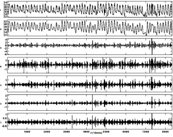
Decompose time series of temperature data can be seen in Fig. 4, using Daubechies wavelet decompose DB4 level 5.
In Table 3, calculation of the estimated error, measurement data is divided into training data and testing data, results analysis wavelet decomposition produces approximation component at each level. Reconstructed approximation generates RMSE minimum for all sub-time series data. Approximate level 1 (A1) is 0.1042 °C/10min for training data. While the RMSE minimum generated by sub-time series Dt+18, Dt+24, Dt+30 for Approximate level 1 (A1) testing data is 0.1370 °C/10min.
Table 3. The RMSE statistics of different sub-time series of observed and wavelet approximation temperature data of Bungus station
Approximate Components RMSE oC/10min Dt+6/Qt Dt+12/Qt Dt+18/Qt Dt+24/Qt Dt+30/Qt A1 0.1042 0.1042 0.1042 0.1042 0.1042 Training A2 0.1792 0.1855 0.1795 0.1855 0.1795 A3 0.2852 0.3021 0.2985 0.2821 0.2850 A4 0.4859 0.4656 0.4648 0.4857 0.4552 A5 0.8421 0.8561 0.8514 0.8343 0.8223 A1 0.1378 0.1375 0.1370 0.1370 0.1370 Testing A2 0.2126 0.2353 0.2118 0.2350 0.2117 A3 0.3317 0.3334 0.3365 0.3352 0.3310 A4 0.5896 0.5455 0.6119 0.5575 0.5672 A5 1.0672 0.9947 1.0913 1.2065 1.2178
While the estimated error data by using MAE shown in Table 4, measurement data using wavelet decomposition analysis produces approximation component at each level. Analysis of the resulting error can be seen with increasing periodic predictions of 1 hour (Dt+6), 2 hours (Dt+12) to 5 hours
(Dt+30) ahead, the resulting error will also increase proportionally in wavelet decomposes level except all level 1 are considered to be consistent. Reconstructed approximation generates MAE minimum for all sub- time series data at approximate level 1 is 0.0719 °C/10min for training data. While the MAE minimum generated by sub-time series Dt + 30 for Approximate level 1 for testing the data was 0.0759 °C/10min.
Table 4. The MAE statistics of different sub-time series of observed and wavelet approximation temperature data of Bungus station
Approximate Components MAE oC/10min Dt+6/Qt Dt+12/Qt Dt+18/Qt Dt+24/Qt Dt+30/Qt A1 0.0719 0.0719 0.0719 0.0719 0.0719 Training A2 0.1199 0.1235 0.1199 0.1235 0.1201 A3 0.1943 0.0913 0.1963 0.1894 0.1940 A4 0.3417 0.3241 0.2161 0.3389 0.3170 A5 0.6286 0.6438 0.7249 0.6359 0.6274 A1 0.0770 0.0768 0.0761 0.0760 0.0759 Testing A2 0.1307 0.1362 0.1294 0.1358 0.1294 A3 0.2056 0.2079 0.2157 0.2170 0.2046 A4 0.4001 0.3770 0.4046 0.3824 0.3780 A5 0.7709 0.7327 0.7919 0.8498 0.8460
From the analysis results in Table 5 using a linear regression to training data sub-time series Dt+6 produces RMSE minimum is 2.5261 °C/10min and MAE is 2.1906 °C/10min, while the maximum 0.0200 R2 was generated by D
t+30. In testing RMSE is 3.0404 °C/10min, MAE is 2.6415 °C/10min, and R2 is 0.0488 to sub-time series of data D
sub-time series Dt+30 became maximum, then error RMSE, MAE will be minimum and R2 will increase in value in the testing data.
Table 5. The RMSE, MAE and R2 statistics of different Linear Regression applications in sub-time series data of Bungus station
Approximate Components Sub-Time Series Dt+6/Qt Dt+12/Qt Dt+18/Qt Dt+24/Qt Dt+30/Qt RMSE 2.5261 2.5277 2.5288 2.5293 0.5295 Training MAE 2.1906 2.1915 2.1917 2.1922 2.1922 R2 0.0154 0.0165 0.0176 0.0188 0.0200 RMSE 3.0830 3.0690 3.0529 3.0419 3.0404 Testing MAE 2.7027 2.6824 2.6623 2.6470 2.6415 R2 0.0387 0.0423 0.0459 0.0484 0.0488
B. ANFIS and Linear Regression Models
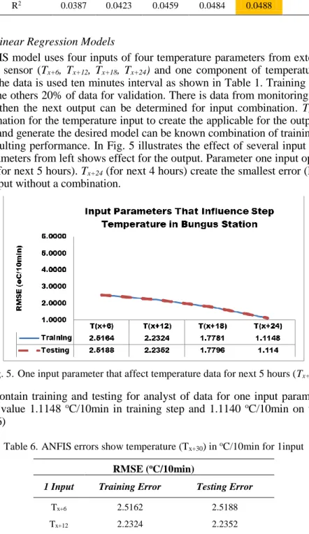
For the ANFIS model uses four inputs of four temperature parameters from extension values of one temperature sensor (Tx+6, Tx+12, Tx+18, Tx+24) and one component of temperature parameter as output (Tx+30). The data is used ten minutes interval as shown in Table 1. Training data use 80% of all of data and the others 20% of data for validation. There is data from monitoring station with 10-minute interval then the next output can be determined for input combination. Tx+30 (5 hours) is optimum combination for the temperature input to create the applicable for the output. By using the ANFIS method and generate the desired model can be known combination of training and validation to obtain the resulting performance. In Fig. 5 illustrates the effect of several input parameters. The sequence of parameters from left shows effect for the output. Parameter one input optimal affects on output of Tx+30 (for next 5 hours). Tx+24 (for next 4 hours) create the smallest error (RSME) to affect output on one input without a combination.
Fig. 5. One input parameter that affect temperature data for next 5 hours (Tx+30)
The results contain training and testing for analyst of data for one input parameter to have the smallest RMSE value 1.1148 oC/10min in training step and 1.1140 oC/10min on testing step (red
colour in Table 6)
Table 6. ANFIS errors show temperature (Tx+30) in oC/10min for 1input
RMSE (oC/10min)
1 Input Training Error Testing Error
Tx+6 2.5162 2.5188
Tx+12 2.2324 2.2352
Tx+18 1.7781 1.7796
In the next phase using 2 input combinations of variables that affect Tx+30 output as shown in Table 7. The optimal value can be reach by combination of Tx+6 and Tx+24. RMSE result 0.9379
oC/10min training value and 0.9390 oC/10min for testing value. The results obtained using ANFIS
method of determining the suitability value of training and testing data by concern average comparable error value.
Table 7. ANFIS errors show temperature (TX+30) in oC/10min for 2 input combinations
RMSE (oC/10min)
2 Input Training Error Testing Error
Tx+6, Tx+12 1.9187 1.9209 Tx+6,Tx+18 1.4693 1.4753 Tx+6,Tx+24 0.9379 0.9390 Tx+12,Tx+18 1.5074 1.5119 Tx+12,Tx+24 0.9420 0.9426 Tx+18,Tx+24 0.9568 0.9549
Table 8 show that training process for 3 inputs, RSME value will increase to 0.9011 oC/10min,
and get value 0.9028 oC/10min in the testing phase. Optimization occurs on the input variable T
x+6,
Tx+18, Tx+24. In this phase, experiment is limited only by using 3 input combinations.
Table 8. ANFIS errors show temperature (TX+30) in oC/10min for 3 input combinations
RMSE (oC/10min)
3 Input Training
Error Testing Error
Tx+6, Tx+12, Tx+18 1.4327 1.4399 Tx+6, Tx+12, Tx+24 0.9171 0.9189 Tx+6, Tx+18, Tx+24 0.9011 0.9028 Tx+12, Tx+18, Tx+24 0.9149 0.9173 C. Analysis Combinations
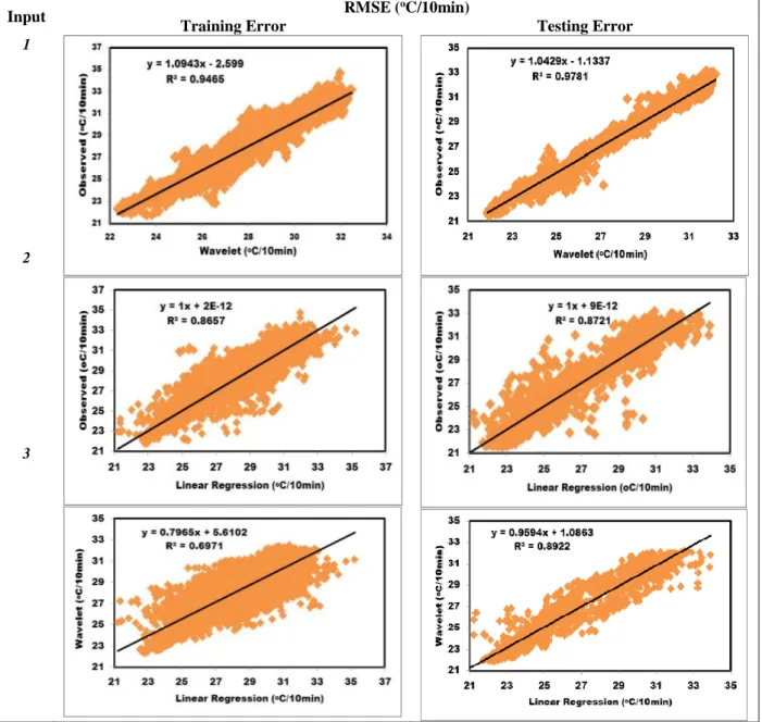
From the above performance of analysis plotting wavelet against observations showing the more optimum value if was compared with other input models. Plotting data input-1 in Fig. 6, the value of data for approximates observed at level 1 (minimum error is the result of sub-time series analysis up to level 5). The combined analysis of data is generated from training and testing.
In Fig. 6, for 1 input, it seen differentiating between real data (Dt+18) with predicted value of Wavelet (approximates), use performance of evaluation criteria such as MEA, RMSE, and R2. Acquired 1 input MAE = 0.4432 °C/10min, R2 = 0.9466, RMSE = 0.6277 °C/10min in training phase, whereas MAE = 0.3193 °C/10min, R2 = 0.9781, RMSE = 0.4789 °C/10min in testing phase. 1 input parameter creates an optimal analysis for temperature output. While for 2 inputs in Fig. 6 are data value observed with linear regression using multiple inputs and single output (minimum error is the result of sub-time series analysis for prediction output). The combined analysis of data is generated from training and testing. For 2 input, it seen differentiating between real data (Dt + 30) and predicted , Acquired of 2 input 2 MAE = 0.6706 °C/10min, R2 = 0.8657, RMSE = 0.9396 °C/ 10min in training phase, whereas MAE = 0.7828 °C/10min, R2 = 0.8721, RMSE = 1.1147 °C/10min in testing phase.
Plotting data for three inputs in Fig. 6, a data value wavelet with linear regression to perform plots for data drawn from analysis of minimum error of each input to each sub-time series of data is generated. The analysis of the data is also generated the training and testing. For 3 Input, it seen differentiating between real data and predicted, acquired 3 input MAE = 0.9564 °C/10min, R2 = 0.6971, RMSE = 1.3389 °C/10min in training phase, whereas MAE = 0.7018 °C/ 0min, R2 = 0.8922,
Input RMSE (
oC/10min)
Training Error Testing Error
1
2
3
Fig. 6. Showing of wavelet model for one input (observed and wavelet), two input combinations (observed and linear regression), three input combinations (wavelet and linear regression) in training and testing
phase.
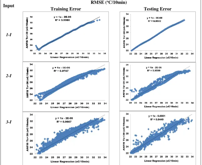
It can be seen the combination of ANFIS model parameters in the training and testing stage that have an effect to get the output, 1 input (Tx+24) and output (Tx+30) with using 100 epoch. In Fig. 7 for 1 input can be seen differentiating between ANFIS and Linear Regression, ANFIS model use performance of evaluation criteria such as RMSE, R2, r. And resulting 1 input r = 0.9994, R2 = 0.9988 RMSE = 0.0807 oC/10min in training phase, and r = 0.9998, R2
= 0.9982, RMSE = 0.0119
oC/10min in testing phase. Use of 1 parameter input is the optimal result in this experiment. The use
of a combination of 2 input parameters at the training and testing phase, the combining affects is (Tx+6 and Tx+24) with Tx+30 output and resulting between 2 models r = 0.9893, R2 = 0.9787 RMSE = 0.3497 oC/10min in training phase, and r = 0.9797, R2
= 0.9599, RMSE = 0.5847 oC/10min in
testing phase. For 3 input parameters at the training and testing phase, the combining affects is (Tx+6,
Tx+18, Tx+24) with Tx+30 output and resulting both of models r = 0.9832, R2 = 0.9667 RMSE = 0.4408
oC/10min in the training phase, and r = 0.9721, R2
= 0.9449, RMSE = 0.6970 oC/10min for the
Input RMSE (
oC/10min)
Training Error Testing Error
1-I
2-I
3-I
Fig. 7. ANFIS model performances on one input (1-I), two input combinations (2-I), three input combinations (3-I) in training and testing phase.
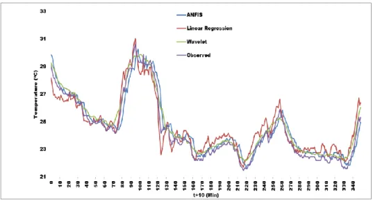
The curve in Fig. 8 and 9 shows the prediction results comparing ANFIS, linear regression and Wavelet. The first line which characterized by a linear regression curve shows the predicted outcome value curve more wide enough from the line of observation. Wavelet line shows output predicted value more wide from line of observation too but closer than linear regression value. While ANFIS predicted curve shows with the one closest to the value of observation and is also characterized by prediction error is minimum than Wavelet and linear regression. Comparison of the results of the data analysis using interval data t(10)min for 350 first data with minimal RMSE comparison.
Fig. 8. The predicted temperature curves of ANFIS, linear regression, wavelet, and observed data (Training Data)
Fig. 9. The predicted temperature curves of ANFIS, linear regression, wavelet, and observed data (Testing Data)
IV. Conclusion
This study uses one weather parameter, temperature, contained in the weather station in Bungus port. The used methods are ANFIS, wavelet and statistical models of linear regression. Statistical indicators such as r,RMSE, MAE, and R2, are calculated for data analysis. The time series data are used to predict next 60 to 300 minutes for 10 minutes data intervals. Data is shared using Mackey Glass Chaotic Time-Series. Wavelet model is used to analyze sub-time series data. Data input was used the result of wavelet decomposes each level. Approximately 8335 pairs of data are divided into training and testing. Approximate value component level 1 error is smaller than the other levels. ANFIS model with multiple input obtained optimum results during training and testing phase. Linear regression analysis using the model is done by multi-input to give one output result of each prediction. Input data of 60, 120, 180, 240 minutes produces output for data prediction for 300 minutes to determine a combination of the output for multi-input for each minute. The analysis was generated using this model is quite well. However, it is not as well as the ANFIS generated prediction. For the input combination, ANFIS against linear regression is the optimal combination performed on this experiment to this research. The application of computational can be combined with more complex models such as Support Vector Machine, Artificial Neural Network, and hope can step over to next experiment with long term and complex data.
References
[1] B. S. Karthika and P. C. Deka, “Prediction of air temperature by hybridized model (Wavelet-ANFIS) using wavelet decomposed data,” Aquat. Procedia, vol. 4, pp. 1155–1161, 2015.
[2] S. Papantoniou and D.-D. Kolokotsa, “Prediction of outdoor air temperature using neural networks: Application in 4 European cities,” Energy Build., vol. 114, pp. 72–79, 2016.
[3] E. Brulebois, T. Castel, Y. Richard, C. Chateau-Smith, and P. Amiotte-Suchet, “Hydrological response to an abrupt shift in surface air temperature over France in 1987/88,” J. Hydrol., vol. 531, pp. 892–901, 2015.
[4] O. Kisi and M. Cimen, “A wavelet-support vector machine conjunction model for monthly streamflow forecasting,” J. Hydrol., vol. 399, no. 1, pp. 132–140, 2011.
[5] K.-C. Hsu and S.-T. Li, “Clustering spatial--temporal precipitation data using wavelet transform and self-organizing map neural network,” Adv. Water Resour., vol. 33, no. 2, pp. 190–200, 2010.
[6] S. J. Yao, Y. H. Song, L. Z. Zhang, and X. Y. Cheng, “Wavelet transform and neural networks for short-term electrical load forecasting,” Energy Convers. Manag., vol. 41, no. 18, pp. 1975–1988, 2000. [7] X. An, D. Jiang, C. Liu, and M. Zhao, “Wind farm power prediction based on wavelet decomposition
and chaotic time series,” Expert Syst. Appl., vol. 38, no. 9, pp. 11280–11285, 2011.
[8] K. Wilgan, W. Rohm, and J. Bosy, “Multi-observation meteorological and GNSS data comparison with Numerical Weather Prediction model,” Atmos. Res., vol. 156, pp. 29–42, 2015.
[9] G. A. Fallah-Ghalhary, M. Mousavi-Baygi, and M. H. Nokhandan, “Annual Rainfall Forecasting by Using Mamdani Fuzzy Inference System,” Res. J. Environ. Sci., vol. 3, no. 4, pp. 400–413, 2009. [10] N. Anwer, A. Abbas, A. Mazhar, and S. Hassan, “Measuring weather prediction accuracy using sugeno
based Adaptive Neuro Fuzzy Inference system, grid partitioniong and guassmf,” in Computing Technology and Information Management (ICCM), 2012 8th International Conference on, 2012, vol. 1, pp. 214–219.
[11] M. Yousefi, D. Hooshyar, A. Remezani, K. S. M. Sahari, W. Khaksar, and F. B. I. Alnaimi, “Short-term wind speed forecasting by an adaptive network-based fuzzy inference system (ANFIS): an attempt towards an ensemble forecasting method,” Int. J. Adv. Intell. Informatics, vol. 1, no. 3, pp. 140–149, 2015.
[12]D. Munandar, "Optimization weather parameters influencing rainfall prediction using Adaptive Network-Based Fuzzy Inference Systems (ANFIS) and linier regression," 2015 International Conference on Data and Software Engineering (ICoDSE), Yogyakarta, 2015, pp. 1-6

![Fig. 2. ANFIS model for two inputs [9]](https://thumb-us.123doks.com/thumbv2/123dok_us/10945330.2983115/4.892.131.725.148.1176/fig-anfis-model-inputs.webp)