Enabling new musical interactions with machine learning

UC San Diego

UC San Diego Electronic Theses and Dissertations

Enabling new musical interactions with machine learning

Permalink https://escholarship.org/uc/item/7zp421mk Author Donahue, Chris Publication Date 2019 Peer reviewed|Thesis/dissertation

UNIVERSITY OF CALIFORNIA SAN DIEGO

Enabling New Musical Interactions with Machine Learning

A dissertation submitted in partial satisfaction of the requirements for the degree

Doctor of Philosophy in Music by Chris Donahue Committee in charge: Miller Puckette, Chair Julian McAuley, Co-Chair Garrison W. Cottrell Shlomo Dubnov Tom Erbe

Copyright Chris Donahue, 2019

The dissertation of Chris Donahue is approved, and it is ac-ceptable in quality and form for publication on microfilm and electronically:

Co-Chair Chair

University of California San Diego 2019

DEDICATION

EPIGRAPH

AI [alone] would have the capacity to write a good song, but not a great one.

TABLE OF CONTENTS

Signature Page . . . iii

Dedication . . . iv Epigraph . . . v Table of Contents . . . vi List of Figures . . . x List of Tables . . . xv Acknowledgements . . . xvii Vita . . . xix

Abstract of the Dissertation . . . xx

I

Introduction

1

1.1 Dissertation organization . . . 6

II

Music generation with machine learning

7

2.1 Musical representations . . . 9

2.2 Music as a factorized probability distribution . . . 11

2.2.1 Discretizing p(music) . . . 12

2.2.2 FactorizingP(music) . . . 12

2.3 Simplifying and generatingP(score) . . . 14

2.3.1 Preserving sequential aspects of music inP(score) . . . 16

2.3.2 Language models forP(score) . . . 19

Chapter 3 Music generation in the symbolic domain . . . 21

3.1 Related work . . . 23

3.2 Dataset preliminaries . . . 24

3.2.1 NES ensemble preliminaries . . . 24

3.3 Representations and tasks . . . 25

3.3.2 Separated score representation and task . . . 26

3.3.3 Event-based representation and task . . . 27

3.3.4 Expressive performance generation . . . 29

3.4 Methodology . . . 30

3.4.1 Transformer architecture . . . 30

3.4.2 Pre-training . . . 31

3.5 Event-based score generation experiments . . . 33

3.5.1 Data augmentation and pre-training . . . 34

3.5.2 Baselines . . . 35

3.5.3 Quantitative analysis . . . 35

3.6 Expressive performance generation experiments . . . 36

3.7 User study . . . 39

3.7.1 Turing test . . . 39

3.7.2 Preference test . . . 41

3.8 Pairing LakhNES with humans . . . 43

3.9 Conclusion . . . 43

3.10 Acknowledgements . . . 43

Chapter 4 Music generation in the acoustic domain . . . 45

4.1 GAN Preliminaries . . . 47

4.2 WaveGAN . . . 48

4.2.1 Intrinsic differences between audio and images . . . 48

4.2.2 WaveGAN architecture . . . 49

4.3 Understanding and mitigating artifacts in generated audio . . . 51

4.3.1 Learned post-processing filters . . . 52

4.3.2 Upsampling procedure . . . 53

4.3.3 Phase shuffle . . . 54

4.4 SpecGAN: Generating semi-invertible spectrograms . . . 55

4.5 Experimental protocol . . . 56

4.6 Evaluation methodology . . . 58

4.6.1 Inception score . . . 58

4.6.2 Nearest neighbor comparisons . . . 59

4.6.3 Qualitative human judgements . . . 60

4.7 Results and discussion . . . 60

4.8 Related work . . . 62

4.9 Improving SpecGAN with adversarial vocoding . . . 64

4.9.1 Summary of contributions . . . 66

4.10 Audio feature preliminaries . . . 66

4.11 Measuring the effect of magnitude and phase estimation on speech naturalness . . . 68

4.12 Adversarial vocoding . . . 69

4.13.1 Vocoding LJ Speech mel spectrograms . . . 74

4.13.2 Unsupervised audio synthesis . . . 76

4.14 Conclusion . . . 77

4.15 Acknowledgements . . . 77

III

New musical interactions

79

5.1 Introduction . . . 81

5.2 Related Work . . . 84

5.3 Methods . . . 84

5.4 Experiments and Analysis . . . 86

5.4.1 Analysis . . . 88

5.5 User Study . . . 91

5.6 Web demo details . . . 92

5.7 Conclusion . . . 93

5.8 Acknowledgements . . . 94

Chapter 6 Dance Dance Convolution . . . 95

6.1 Introduction . . . 95 6.1.1 Contributions . . . 99 6.2 Data . . . 100 6.3 Problem Definition . . . 101 6.4 Methods . . . 103 6.4.1 Audio Representation . . . 103 6.4.2 Step Placement . . . 104 6.4.3 Peak Picking . . . 106 6.4.4 Step Selection . . . 107 6.5 Experiments . . . 109 6.5.1 Step Placement . . . 109 6.5.2 Step Selection . . . 111 6.6 Discussion . . . 112 6.7 Related Work . . . 114 6.8 Conclusions . . . 116 6.9 Acknowledgements . . . 116

Chapter 7 Other interactive systems . . . 117

7.1 DrumGAN . . . 117

7.2 Neural Loops . . . 119

7.3 Semantically-decomposed GANs . . . 121

LIST OF FIGURES

Figure 1.1: Piano improvisation is a task hitherto inaccessible by non-musicians despite many having the potential capacity. This task combines high-level musical intuition with lower-level planning and mechanical expertise. Could we relax (Chapter 5) or one day circumvent (dashed line) the intermediate steps which currently prevent non-musicians from expressing their dormant musical intuition through the piano? . . . 3 Figure 2.1: Symbolic (left) and acoustic (right) representations of the same piece of

music (Prelude in C major, BWV 846, J. S. Bach). Sheet musicis a symbolic format most familiar to musicians.MIDIstores all of the information about a composition in a compact list of musical events. Piano rollencodes MIDI information into a time-pitch grid retaining the relationships between notes.

Waveforms (recordings) are a digital representation of a musical pressure wave. Spectrograms are a time-frequency decomposition of waveforms which resemble how the human auditory system processes sound that arrives at our ears. . . 10 Figure 2.2: Comparing the pitch class frequencies for specific pieces composed by Bach

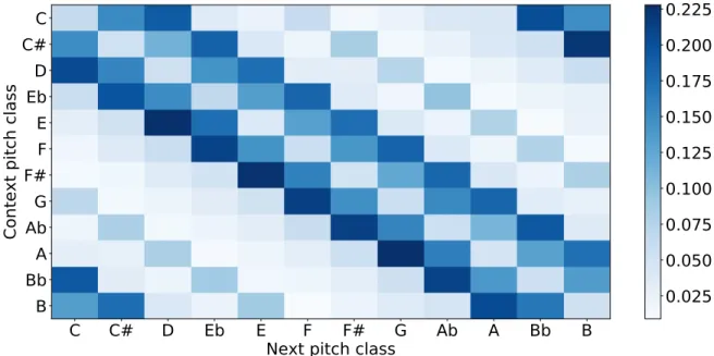
and Sch¨onberg. . . 14 Figure 2.3: Pitch class transition likelihoods across all of Bach’sWell-Tempered Clavier

(BWV 846–893). The transitions reflect our understanding of Bach’s compo-sitional style. For example, major seconds are the most likely intervals while tritones are the least likely. . . 17 Figure 2.4: Trigram, 4-gram, and 5-gram models for Bach’s Well-Tempered Clavier.

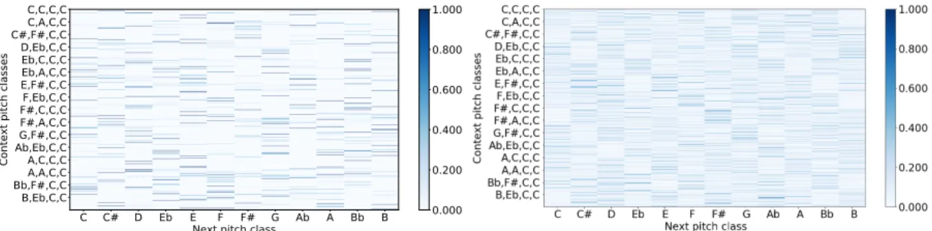
While the exponential growth of the model parameters make it difficult to interpret the distributions visually, we can see that the sparsity of the models (how manyn-grams werenotpresent in the corpus) increases as the context grows (i.e., there is more whitespace in the diagram). . . 18 Figure 2.5: Comparing likelihoods assigned to sequences of five pitch classes by a

5-gram distribution (left) and a recurrent neural network (right) trained on the same corpus. The recurrent neural network has learned a smooth parameteri-zation of the distribution that allows us to estimate reasonable likelihoods for sequences which did not appear in the training data. . . 19 Figure 3.1: Four representations for a segment ofEnding ThemefromAbadox(1989)

by composer Kiyohiro Sada. The blended score (fig. 3.1a), used in prior polyphonic generation research, is degenerate when multiple voices play the same note. . . 25

Figure 3.2: A visual comparison between the piano roll representation of the original NES-MDB paper [Donahue et al., 2018c] (top) and the event representation of this work (bottom). In the piano roll representation, the majority of information is the same across timesteps. In our event representation, each timestep encodes a musically-meaningful change. . . 28 Figure 3.3: Illustration of our mapping heuristic used to enable transfer learning from

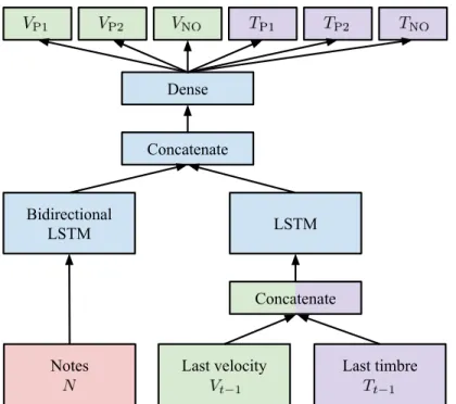
Lakh MIDI to NES-MDB. We identify monophonic instruments from the arbitrary ensembles in Lakh MIDI and randomly assign them to the fixed four-instrument ensemble of NES-MDB. . . 32 Figure 3.4: LSTM Note+Auto expressive performance model that observes both the

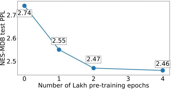
score and its prior output. . . 38 Figure 3.5: Measuring the performance improvement when doubling the amount of Lakh

MIDI pre-training before fine-tuning Transformer-XL on NES-MDB. Each datapoint represents the result of a fine-tuning run starting from 0, 1, 2, or 4 epochs of Lakh MIDI pre-training. Additional amounts of pre-training appear to improve performance, though with diminishing returns. . . 40 Figure 3.6: Human accuracy at distinguishing computer-generated examples from

human-composed ones (error bars are standard error). Users were presented with pairs of clips (one human, one computer) and tasked with identifying which was composed by a human. Random examples are used as a control and we filtered annotators with accuracy less than 1 on those pairs. Aloweraccuracy is better as it indicates that the annotators confused a particular model with the real data more often. . . 41 Figure 3.7: Proportion of comparisons where humans preferred an example from each

model over an example from another random model (error bars are standard error). Users were presented with pairs of clips from different methods and asked which they preferred. Pairs of random data and human-composed clips are used as a control and we filtered annotators who preferred random. A

higherratio is better as it indicates that the annotators preferred results from that method more often than another. . . 42 Figure 4.1: First eight principal components for 5x5 patches from natural images (left)

versus those of length-25 audio slices from speech (right). Periodic patterns are unusual in natural images but a fundamental structure in audio. . . 49 Figure 4.2: Depiction of the transposed convolution operation for the first layers of

the DCGAN [Radford et al., 2016] (left) and WaveGAN (right) generators. DCGAN uses small (5x5), two-dimensional filters while WaveGAN uses longer (length-25), one-dimensional filters and a larger upsampling factor. Both strategies have the same number of parameters and numerical operations. 50

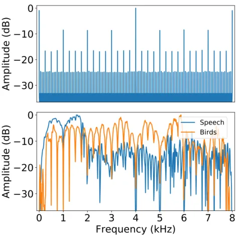
Figure 4.3: (Top): Average impulse response for 1000 random initializations of the WaveGAN generator. (Bottom): Response of learned post-processing filters for speech and bird vocalizations. Post-processing filters reject frequencies corresponding to noise byproducts created by the generative procedure (top). The filter for speech boosts signal in prominent speech bands, while the filter for bird vocalizations (which are more uniformly-distributed in frequency) simply reduces noise presence. . . 52 Figure 4.4: Depiction of the upsampling strategy used by transposed convolution (zero

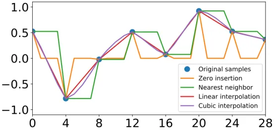
insertion) and other strategies which mitigate aliasing: nearest neighbor, linear and cubic interpolation. . . 53 Figure 4.5: At each layer of the WaveGAN discriminator, the phase shuffle operation

perturbs the phase of each feature map by Uniform∼[−n,n]samples, filling in the missing samples (dashed outlines) by reflection. Here we depict all possible outcomes for a layer with four feature maps (n=1). . . 54 Figure 4.6: Top: Random samples from each of the five datasets used in this study,

illustrating the wide variety of spectral characteristics. Middle: Random samples generated by WaveGAN for each domain. WaveGAN operates in the time domain but results are displayed here in the frequency domain for visual comparison. Bottom: Random samples generated by SpecGAN for each domain. . . 56 Figure 4.7: Depiction of stages in common audio feature extraction pipelines and

cor-responding inversion. The two obstacles to vocoding are (1) estimating linear-frequency magnitude spectra from log-frequency mel spectra (outlined in green dashed line), and (2) estimating phase information from magnitude spectra (outlined in blue dotted line). We focus on magnitude estimation in this paper, observing that coupling an ideal solution to this subproblem with a phase estimation heuristic can produce high-quality speech (Table 4.2). . 67 Figure 4.8: Adversarial Vocoder Model: The generator performs an image-to-image

translation from the estimated magnitude spectrogram to the actual magnitude spectrogram guided by an adversarial loss from the discriminator and theL₁

distance between the generated and actual magnitude spectrogram . . . 72 Figure 5.1: Using Piano Genie to improvise on a Disklavier (motorized piano) via MIDI. 82 Figure 5.2: Piano Genie consists of a discrete sequential autoencoder. A bidirectional

RNN encodes discrete piano sequences (88 keys) into smaller discrete latent variables (8 “buttons”). The unidirectional decoder is trained to map the latents back to piano sequences. During inference, the encoder is replaced by a human improvising on buttons. . . 83

Figure 5.3: Comparison of the quantization scheme for two autoencoder strategies with discrete latent spaces. The VQ-VAE (left) learns the positions ofkcentroids in a d-dimensional embedding space (in this figure k=8,d =2, in our experimentsk=8,d=4). An encoder output vector (grey circle) is quantized to its nearest centroid (yellow circle) before decoding. Our IQAE strategy (right) quantizes a scalar encoder output (grey) to its nearest neighbor (yellow) amongk=8 centroids evenly spaced between−1 and 1. . . 85 Figure 5.4: Qualitative comparison of the 8-button encodings for a given melody (top)

by the VQ-VAE (middle) and our IQAE withL_contour (bottom). Horizontal is note index. The encoding learned by the IQAE echoes the contour of the musical input. . . 89 Figure 5.5: A user engages with the Piano Genie web interface during our user study. . 90 Figure 6.1: Proposedlearning to choreographpipeline for four seconds of the songKnife

Party feat. Mistajam - Sleaze. The pipeline ingests audio features (Bottom) and produces a playable DDR choreography (Top) corresponding to the audio. 96 Figure 6.2: A four-beat measure of a typical chart and its rhythm depicted in musical

notation. Red: quarter notes,Blue: eighth notes,Yellow: sixteenth notes,

(A):jumpstep,(B):freezestep . . . 98 Figure 6.3: Five seconds of choreography by difficulty level for the songKOAN Sound

-The Edgefrom the Fraxtil training set. . . 100 Figure 6.4: Number of steps per rhythmic subdivision by difficulty in the Fraxtil dataset. 102 Figure 6.5: C-LSTM model used for step placement . . . 104 Figure 6.6: One second of peak picking. Green: Ground truth region(A): true positive,

(B): false positive,(C): false negative,(D): two peaks smoothed to one by Hamming window,(E): misaligned peak accepted as true positive by±20ms

tolerance . . . 107 Figure 6.7: LSTM model used for step selection . . . 108 Figure 6.8: Top: A real step chart from theFraxtildataset on the songAnamanaguchi

-Mess. Middle: One-step lookaheadpredictionsfor the LSTM model, given Fraxtil’s choreography as input. The model predicts the next step with high accuracy (errors in red). Bottom: Choreography generated by conditional LSTM model. . . 113 Figure 7.1: Interface for a demo of DrumGAN, which combines a WaveGAN generative

model of drum one-shots with a traditional step sequencer. . . 118 Figure 7.2: The interface forNeural Loops, which combines multiple neural network

gen-erative models with a traditional musical sequencer to produce an interactive tool for exploring four-bar musical trios. . . 120 Figure 7.3: Schematic diagram forNeural Loopsillustrating the generative models used

Figure 7.4: The factorized latent spaces of semantically-decomposed generative adver-sarial networks allow for independent manipulation of salient and contingent aspects of multimedia such as face portraits and visual artworks. . . 122

LIST OF TABLES

Table 3.1: Schematic for our event-based representation of NES-MDB, reminiscent of the one used inPerformance RNN[Simon and Oore, 2017]. The 631 events in our representation are distributed among time-shift (∆T) events (which allow

for nuanced timing), and note off/on events for individual instruments (as in typical MIDI). . . 29 Table 3.2: Quantitative performance of various models trained on the event-based

rep-resentation (631 event types) of NES-MDB.Paramsindicates the number of parameters of each model. Epochsis the number of data epochs the model observed before early stopping based on the validation data. Test PPL repre-sents the perplexity of the model on the test data, i.e., the exponentiation of its average negative log-likelihood on the test data. Alowerperplexity indicates that the modelbetterfits this unseen data. . . 35 Table 3.3: Results for expressive performance experiments evaluated at points of interest

(POI). Results are broken down by expression category (e.g. V_NO is noise velocity,T_P1 is pulse 1 timbre) and aggregated at POIs and globally (All). . . 37 Table 4.1: Quantitative and qualitative (human study) results for SC09 experiments

comparing real and generated data. A higher inception score suggests that semantic modes of the real data distribution have been captured. |D|_self

indicates the intra-dataset diversity relative to that of the real test data.|D|train

indicates the distance between the dataset and the training set relative to that of the test data; a low value indicates a generative model that is overfit to the training data. Acc. is the overall accuracy of humans on the task of labeling class-balanced digits (random chance is 0.1). Soundquality,easeof intelligibility and speakerdiversityare mean opinion scores (1-5); higher is better. . . 61 Table 4.2: Ablating the effect of heuristics for magnitude and phase estimation on mean

opinion score (MOS) of speech naturalness with 95% confidence intervals.

Boldedentries show that coupling an ideal solution to either subproblem (real data used as a proxy) with a good heuristic for the other yields speech with only 2–9% lower MOS than real speech (p<0.05). . . 69 Table 4.3: Comparison of vocoding methods on mel spectrograms with 80 bins. We

display comparative mean opinion scores from two separate user studies for vocoding spectrograms extracted from real speech (MOS-Real) and spectro-grams generated by a state-of-the-art TTS method (MOS-TTS) with 95% confidence intervals. × RT denotes the speed up over real time; higher is faster. MB denotes the size of each model in megabytes. . . 75 Table 4.4: Comparison of heuristic and adversarial vocoding of spectrograms with

Table 4.5: Combining our adversarial vocoding approach with GAN-generated mel spec-trograms outperforms our prior work in unsupervised generation of individual

words by all metrics. . . 76

Table 5.1: Quantitative results comparing an RNN language model, the VQ-VAE (k= 8,d=4), and our proposed IQAE model (k=8) with and without contour regularization.∆T adds time shift features to model. PPL is perplexity: eLrecons_. CVR is contour violation ratio: the proportion of timesteps where the sign of the melodic interval6=that of the button interval. Gold is the mean squared error in button space between the encoder outputs for familiar melodies and manually-created gold standard button sequences for those melodies. Lower is better for all metrics. . . 87

Table 5.2: Results for a small (n=8) user study for Piano Genie. Partipicants were given up to three minutes to improvise on three possible mappings between eight buttons and an 88-key piano: 1) (G-maj) the eight buttons are mapped to a G-major scale, 2 (language model) all buttons trigger our baseline language model, 3 (Piano Genie) our proposed method. (Time) is the average amount of time in seconds that users improvised with a mapping. (Per.,Mus.,Con.) are the respective averages users expressed for enjoyment of performance experience, enjoyment of music, and level of control. . . 90

Table 6.1: Dataset statistics . . . 101

Table 6.2: Results for step placement experiments . . . 109

ACKNOWLEDGEMENTS

Thanks to my Committee Chair Miller Puckette for his unconditional support throughout my PhD. His input was central to the success of my research projects despite several of them being outside his primary area of expertise. It is impossible to overstate my indebtedness to my Co-chair Julian McAuley, who offered me a level of guidance far beyond the call of a faculty member and molded me from a tinkerer into a researcher. Additional thanks to all of the members of my committee for their support and encouragement throughout my postgraduate studies.

I am indebted to Zachary C. Lipton, who guided me with remarkable patience through the process of publishing my first machine learning papers. Thanks to Nicolas Boulanger-Lewandowski at Google, who accepted me as an intern despite my inexperience, and set me along my current research path. Thanks to Stephen Burnaman and Terry McKinney for teaching me everything I know about musicianship. Thanks to Russell Pinkston, Ethan Greene, and Peter Stone who got me started on all of this computer music business.

My deepest thanks to my parents, Linda and Jim, for their continued love and support—I am incredibly lucky to have been raised by them. Thanks to my brother Jeff for his moral support and research guidance. Thanks to Maggie Henderson for being a constant source of respite during this rollercoaster ride known as a “PhD” and beyond.

Thank you to all of my friends here in San Diego and across the globe who have kept me sane throughout the process (to name a few): Abhay Agarwal, Adam Sydnor, Alex Forsythe, Andrew Elrod, Annie Hui-Hsin Hsieh, Ashvin Bashyam, Carolyn Yuan, Celeste Oram, Cheng-i Wang, Colin Zyskowski, Collin Buchan, Eric Lyday, Gabe Garcia, Jayhee Min, Jeff Sun, Jen Hsu, Johannes Regnier, Keir GoGwilt, Kevin Cannon, Kevin Haywood, Nick Kubala, Niko Millias, Paulina Hensman, Rachel Cassidy, Ryan Done, Ryan Sema, and Sam Asinof.

Thank you to all of my co-authors whose input and guidance was crucial to my research success to date (in chronological order): Tom Erbe, Miller Puckette, Zachary C. Lipton, Julian

Shuo Chen, Ishaan Gulrajani, Adam Roberts, Ian Simon, Sander Dieleman, Paarth Neekhara, Shlomo Dubnov, Yiting Ethan Li, and Garrison W. Cottrell.

Chapter 3 contains material found in the following two papers. (1) The NES Music Database: A multi-instrumental dataset with expressive performance attributes. 2018. Mao, Huanru Henry; McAuley, Julian. International Society for Music Information Retrieval 2018. (2)LakhNES: Improving multi-instrumental music generation with cross-domain pre-training. 2019. Mao, Huanru Henry; Li, Yiting Ethan; Cottrell, Garrison W.; McAuley, Julian. Currently under review for publication. The dissertation/thesis author was the primary investigator and author of these papers.

Chapter 4 contains material found in the following two papers. (1)Adversarial audio synthesis. 2018. McAuley, Julian; Puckette, Miller. International Conference on Learning Repre-sentations 2019. (2)Expediting TTS synthesis with adversarial vocoding. 2019. Neekhara, Paarth; Puckette, Miller; Dubnov, Shlomo; McAuley, Julian. Currently under review for publication. The dissertation/thesis author was the primary investigator and author of these papers.

Chapter 5, in full, is a reprint of the material as it appears inPiano Genie. 2019. Simon, Ian; Dieleman, Sander. ACM conference on Intelligent User Interfaces 2019. The disserta-tion/thesis author was the primary investigator and author of this paper.

Chapter 6, in full, is a reprint of the material as it appears inDance Dance Convolution. 2017. Lipton, Zachary C.; McAuley, Julian. International Conference on Machine Learning 2017. The dissertation/thesis author was the primary investigator and author of this paper.

VITA

2013 B. S. in Computer Science, The University of Texas at Austin 2016 M. A. in Music, University of California San Diego

2019 Ph. D. in Music, University of California San Diego

PUBLICATIONS

Chris Donahue, Ian Simon, Sander Dieleman. “Piano Genie”,ACM Conference on Intelligent User Interfaces, 2019.

Chris Donahue, Julian McAuley, Miller Puckette. “Adversarial audio synthesis”,International Conference on Learning Representations, 2019.

Jesse Engel, Kumar Krishna Agrawal, Shuo Chen, Ishaan Gulrajani, Chris Donahue, Adam Roberts. “GANSynth: Adversarial neural audio synthesis”,International Conference on Learning Representations, 2019.

Chris Donahue, Huanru Henry Mao, Julian McAuley. “The NES Music Database: A multi-instrumental dataset with expressive performance attributes”,International Society for Music Information Retrieval, 2018.

Chris Donahue, Zachary C. Lipton, Akshay Balsubramani, Julian McAuley. “Semantically decomposing the latent spaces of generative adversarial networks”,International Conference on Learning Representations, 2018.

Chris Donahue, Bo Li, Rohit Prabhavalkar. “Exploring speech enhancement with generative adversarial betworks for robust speech recognition”, International Conference on Acoustics, Speech, and Signal Processing, 2018.

Chris Donahue, Zachary C. Lipton, Julian McAuley. “Dance Dance Convolution”,International Conference on Machine Learning, 2017.

Chris Donahue, Tom Erbe, Miller Puckette. “Extended convolution techniques for cross-synthesis”,International Computer Music Conference, 2016.

ABSTRACT OF THE DISSERTATION

Enabling New Musical Interactions with Machine Learning

by

Chris Donahue

Doctor of Philosophy in Music University of California San Diego, 2019

Miller Puckette, Chair Julian McAuley, Co-Chair

Despite the ubiquity of computers leading to a steady increase in global music consump-tion, computing has yet to fundamentally transform the capacity for non-musicians to engage with music. The experience of non-musicians—that of passively listening to music—is largely the same as it was decades prior. In this dissertation, I describe my research which allows non-musicians and musicians alike to create, respond, modify, or otherwiseinteractwith music in new ways. Examples include a system which allows non-musicians to improvise on musical instruments without experience, and a system which automatically choreographs music to provide an interactive listening and dancing experience.

Common to all of my work is the use of predictive models which allow us to efficiently sift through musical spaces to identify promising content. The identified content can then be further curated by humans as part of an interactive musical workflow. To build such predictive models, I use machine learning which seeks to extract and generalize patterns in human-composed music. Specifically, I focus on a subfield of machine learning called deep learning, which is capable of extracting such patterns in high-dimensional music representations including both symbolic and acoustic formats. My research focuses on both advancing the state of the art in deep learning for music (and other types of multimedia), and designing interfaces which allow humans to intuitively benefit from what deep learning systems have discovered about music.

Part I

Chapter 1

Introduction

The primary goal of my research is to build systems which allow people tointeractwith music in new ways. By “interact”, I am referring broadly to any type of engagement with music apart from passive listening, i.e., normal listening experiences for musical recordings. New interactive systems could allow hitherto passive listeners toactivelyengage with or manipulate music they are listening to, or perhaps even create music themselves. In practice, my recent work has focused on augmenting the creative music capacity of humans by designing interfaces which allow them to pilot or curate generative music systems trained using machine learning. For non-musicians, interactive machine learning systems can lower the barrier to entry for music creation by allowing them to intuitively express their musical ideas. For musicians, such systems expedite laborious sub-tasks of digital music production (e.g. selecting a sample from a sample library) by designing interfaces which allow for efficient exploration.

Typical systems for creating music (e.g. musical instruments, sheet music, digital audio workstations) are complex and require high levels of musical expertise for desirable operation. Such expertise eludes the vast majority of the population because acquiring it requires substantial time and financial commitments. Accordingly, the prerequisite capacity and intuition for musical expression lies dormant in many non-musicians. A goal of my research is to build systems which

Musical intuition

Musical language

Precise actions

Piano interface

?

High-level

Low-level

Figure 1.1: Piano improvisation is a task hitherto inaccessible by non-musicians despite many having the potential capacity. This task combines high-level musical intuition with lower-level planning and mechanical expertise. Could we relax (Chapter 5) or one day circumvent (dashed line) the intermediate steps which currently prevent non-musicians from expressing their dormant musical intuition through the piano?

allow for intuitive expression of musical ideas but do not require traditional forms of musical expertise.

To unpack the obstacles to building such systems, let’s examine the practice of improvising on the piano. This task can be oversimplified into the following procedure (Figure 1.1). First, the improviser must mentally formulate their piece using theirmusical intuition. Then, perhaps implicitly, these ideas are translated into the discrete “language” of music, i.e., sequences of rhythms and pitches. Finally, this musical language must be translated into a precise series of physical actions that the performer inputs into the piano interface in real-time.

Arguably, much of the beauty and higher-level reasoning involved in piano improvisa-tion resides in the first step of conceiving a piece from one’s musical intuiimprovisa-tion. However, a disproportionate amount of the effort involved in learningto play the piano is on building the lower-level planning and dexterity required to precisely impart those ideas onto the keys. Of course, years of formal piano instruction also help to shape one’s high-level musical intuition. But could we possibly decouple the development of these high-level skills from the low-level

skills required to precisely input musical patterns on particular instruments? Could we create systems which circumvent these intermediate steps (dashed line Figure 1.1), allowing performers to translate their musical ideasdirectlyinto the piano? Such systems would disentangle musical intuition from mechanical expertise, providing a means for people to express the former without learning the latter. Directly translating signals from the brain into the piano remains science fiction, however later in this dissertation I will discuss a physical interface which achieves this high-level goal to a degree.

A separate issue with modern music creation systems (e.g. digital audio workstations) is that many common tasks are extremely laborious. For example, an electronic music producer might spend large amounts of time scouring endless directories of audio clips in search of the perfect kick drum sound for her track. She might also spend inordinate amounts of time manually adjusting the volume and timing of a drum pattern to achieve a desired effect. Can we design interfaces which allow musicians to quickly explore a trove of reasonable outcomes for such routine tasks? By transforming laborious manual tasks into efficient exercises in exploration and curation, such systems would augment the productivity of existing musicians.

All of the systems I have described so far involve making predictions on behalf of humans. As such, they requirepredictive models that can make musical decisions similarly to human experts. In my research, I use machine learning to build such models. Machine learning systems extract patterns from human-composed music which can then be used to make predictions for new data and offer state-of-the-art performance for a wide variety of musical prediction tasks. I will detail systems I built which can synthesize attributes of music in a variety of different contexts, from simpler tasks like creating expressive dynamics to more complex tasks like generating waveforms.

Machine learning (ML) systems for music suffer two primary drawbacks. The first is that the tooling infrastructure for training such systems is highly inaccessible, requiring extensive

effort—it is possible to package models trained in this unfriendly environment into familiar musical interfaces complete with knobs and faders. The second drawback is that ML systems are (currently) frail and largely incapable of high-level musical decision making. Luckily, it is possible through human-computer interfaces to pair the high-level planning abilities of humans (e.g. writing a chord progression for a song) with the efficiency of ML systems for low-level tasks (e.g. producing hundreds of reasonable melodies given a chord progression). Hence, a sizable portion of my research involves building and evaluating interfaces between people and predictive music systems.

At this point I hope to preemptively address a common criticism of my work. Namely, that building systems which lower the barrier to entry for music creation will cheapen the experience of existing musicians. This is not the case as existing musicians will always have the advantage of stronger musical intuition acquired through years of practice. Hence, musicians will always have higher capacity for precise creative expression regardless of the musical tooling available.

As we enter the era of artificially intelligent (AI) music systems, I believe strongly that humans must be kept in the loop. Beyond the aforementioned practical rationale, there are many other reasons why this is the case. I struggle to envision a future where computers are writing music for other computers, so human ears will continue to be the intended recipients. Hence, humans will always be the toughest critic and the only real ground truth for evaluating AI music systems. Additionally, no matter how compelling the music produced by an AI system is, ultimately I believe that humans will always have the advantage when it comes to true creativity, rather than just mimicking that which came before. My vision of AI is that, like electronics before it, it becomes yet another tool in our musical toolbox allowing for deeper musical expression.

1.1

Dissertation organization

I begin this dissertation with an extended discussion in Part II of my work on using machine learning to build generative models of music at both the symbolic and acoustic level. Chapter 2 provides an explanation of modeling music as a probability distribution, which will be central to the developments of the rest of the thesis. Chapter 3 will discuss the generation of discrete musical scores (i.e. symbolic representations of music), and Chapter 4 will discuss the generation of musical (and other types of) waveforms (i.e. acoustic representations of music).

In Part III, I describe my research on building systems which allow for new musical inter-actions with a focus on co-creation between humans and generative models of music. Chapter 5 will discuss my work on lowering the barrier to entry for playing musical instruments with ma-chine learning. Chapter 6 will present a system which allows non-musicians to interact with their personal music collection through a dance-based video game. Chapter 7 contains information about other demos I have built which merge traditional music interfaces such as sequencers with powerful generative models of music. In Part IV, I offer some concluding remarks.

Part II

Chapter 2

Preliminaries

In this chapter I describe methodology that I have developed for buildingmusic generation

systems with machine learning. As previously stated, my ultimate goal is to build machine learning systems which allow humans to interact with music in new ways. However, in this portion of my dissertation I focus exclusively on the machine learning methodology I have developed towards this goal, and discuss how humans can benefit from this work in Part III.

Machine learning (ML) systems extract patterns from collections of natural data in order to make predictions about the natural world. ML is most appropriate for tasks where it would be difficult to manually program a function to accomplish a particular goal. For example, it would be appropriate to use ML to recognize chord progressions from recordings of music. However, it would be less appropriate to use ML to identify a key signature from MIDI data, as a simple heuristic based on the prevalance of particular pitch classes would suffice.

A particular area of machine learning calleddeep learninghas recently been increasing in popularity because of its ability to model and make predictions about high-dimensional data [Le-Cun et al., 2015]. Music is inherently high-dimensional data with rich structure; accordingly, deep learning is my tool of choice for the predictive tasks I encounter in my research. The goal of deep learning is to train neural networks—non-linear functions often with millions of parameters—to

map data from one domain to another. In a typical setting, a neural network is trained to perform asupervisedlearning task, e.g. labeling data. To accomplish this, data is passed into the neural network which returns estimates for the likelihood of particular labels. These estimates are compared to the real labels, and the error of the estimates is used to improve the parameters of the neural network, in a process known asbackpropagation[Rumelhart et al., 1985].

Unlike in other domains such as image and speech recognition where deep learning dominates, labeled data is a scarce resource in music. Additionally, the objectives in applying machine learning to music are often less clear than the objectives of applying machine learning to e.g. speech recognition. Hence, in my research I also explore unsuperviseddeep learning approaches, where the goal is to train neural networks to recognize patterns in unlabeled data. For example, could we recognize commonalities across the hundreds of four-voice chorales composed by J.S. Bach? Often, my goal with using unsupervised learning is togeneratenew music in the style of the training data, hence I refer to these approaches as generative modeling. Could we extrapolate the patterns we extracted from Bach’s chorales to generate convincing chorales in his style?

Because I seek to generatemusic, the majority of Part II will focus on unsupervised learning strategies. In Chapter 3, I will discuss methodology for learning to generate music in the symbolic domain. In Chapter 4, I will discuss music generation in the acoustic domain. First, I offer an explanation of both musical representations and treating music as a probability distribution which will inform later methodology.

2.1

Musical representations

Of considerable importance to the development of machine learning methodology for music is the choice ofinput representation. Here, input representation refers to how music data is presented to a neural network. As a coarse taxonomy, music representations can be divided into

Symbolic

(discrete)

Acoustic

(continuous)

Waveforms

Spectrograms

Sheet music

MIDI

Piano roll

Figure 2.1: Symbolic (left) and acoustic (right) representations of the same piece of music (Prelude in C major, BWV 846, J. S. Bach).Sheet musicis a symbolic format most familiar to musicians.MIDIstores all of the information about a composition in a compact list of musical events.Piano rollencodes MIDI information into a time-pitch grid retaining the relationships between notes.Waveforms(recordings) are a digital representation of a musical pressure wave.

Spectrogramsare a time-frequency decomposition of waveforms which resemble how the human auditory system processes sound that arrives at our ears.

two categories: symbolicandacoustic(Figure 2.1). Symbolic representations are any strategy which represents music as discrete data, such that it could straightforwardly be engraved as sheet music. Common symbolic representations include MIDI and piano roll. Acoustic representations are any strategy which captures an audio waveform, such that it could be easily be played out of a loudspeaker. Common acoustic representations include time-domain waveforms and frequency-domain spectrograms.

The choice between symbolic and acoustic representations is one of many trade-offs. For example, we might intuitively gravitate towards symbolic music representations for music generation tasks, because they more compactly represent a composer’s intentions than acoustic representations. Such a choice has its limitations however, as symbolic music data is far less common than acoustic music data. Hence, we might seek to generate music by modeling music in the audio domain, but this makes the task much more complicated because audio waveforms are high-dimensional and also entangle information about the underlying composition with information about a particular acoustic performance. Additionally, the choice of representation has implications for both the tasks that we can investigate and the types of neural networks that we can use to model the music in our chosen representation. Therefore, an input representation would be selected to match a particular task and methodology, or vice versa.

2.2

Music as a factorized probability distribution

An assumption that underlies all of the methodological contributions here is that music can be modeled as a probability distribution, and that any given piece of music can be viewed as a sample from this distribution. A probability distribution is a function that maps all possible configurations of sources of randomness (random variables) into a number which specifies how “likely” that configuration is. Henceforth I will refer to the hypothetical distribution of music as

that each of them would be sampled from the distribution with equal likelihood. Whether or not you agree philosophically with this definition, please consider it a conceit that we will use to build and understand generative models of music.

In this context, p(music)encapsulates all of the random factors that can affect a time-varying pressure signal which arrives at a human ear and is described by at least one person in the world as “music”. A random sample from this distribution is a real-valued, time-varying pressure signal with unbounded length. Never in my work do I attempt to directly model this probability distribution. Instead, I “fix” certain random factors to construct regions of this distribution which I can tractably model. First, I describe an important simplifying assumption.

2.2.1

Discretizing

p

(

music

)

An important simplifying assumption I make is that music has been sampled at discrete points in time and its pressure (amplitude) has been quantized. I will refer to this distribution asP(music), where the capital letter is used to signify the discrete nature of samples from this probability distribution (as opposed to the continuous samples of p(music). Hence, a sample from this distributionmmm∈_ZN_{∼P(music)is a vector ofN(variable-length) samples with quantized}

amplitude values in set_Zand a sampling frequency f_s. A single discrete samplemmm∼P(music)

represents an infinite number of continuous samples from p(music). However, I make an assumption that humans would not be able to tell the difference between these infinite continuous samples given standard configurations of fs andZ(e.g. 44.1kHz, 16-bit audio), and hence the

discrete samplemmmis sufficient to represent them.

2.2.2

Factorizing

P

(

music

)

P(music)encapsulates every source of randomness that can affect a digital musical wave-form. To name a few possible sources: composer, performer, ensemble, instrument, microphone,

temperature, composer’s mood, length of time the ensemble played for, how much coffee the drummer had, etc. Hence, we canfactorizethis distribution by fixing certain random factors and modeling the remaining ones.

To determine which factorizations are reasonable, we turn to both our knowledge of how music arises naturally and the data we have available. For example, we know that some types of music arise from different performers playing the same score. Hence, we might factorize as

P(music) =P(score)·P(acoustic realization|score). This is a flexible approach that allows us to independently explore generative methods for musicscoreand musicperformance. We might also only have data available for a specific composer, and thus by using their compositions as training data, we are implicitly modelingP(score|composer=Bach).

We know that an acoustic realization of a score also involves several factors. Hence, we simplify further to the following factorization

P(music) =P(score)·P(performance|score)·P(acoustic|performance). (2.1) In this factorization,scorerefers to all of the attributes necessary to engrave a piece of music as sheet music (Figure 2.1). Performancerefers to all of the expressive performance attributes such as dynamics and rubato which a skilled performer uses when performing a rendition. Finally,

acousticrefers to the acoustic properties that yield a waveform from a performance such as the timbre of the instruments, the room configuration, and the microphone used.

This factorization is convenient to work with because it allows us to examine each portion of this generative music “pipeline” independently. We can develop, for example, mix-and-match various methods of generating scores with methods for generating performances from scores. Throughout the remainder of Part II, I will discuss methods that pertain to the various com-ponents of Equation (2.1). In Chapter 3, I will discuss a neural network pipeline modeling

represent-C represent-C# D Eb E F F# G Ab A Bb B 0.00 0.05 0.10 0.15 0.20 0.25 Likelihood

Pitch class likelihoods from Bach BWV 486 (Prelude)

C C# D Eb E F F# G Ab A Bb B 0.00 0.05 0.10 0.15 0.20 0.25 Likelihood

Pitch class likelihoods from Schönberg op. 33

Figure 2.2: Comparing the pitch class frequencies for specific pieces composed by Bach and Sch¨onberg.

ingP(acoustic|performance). In Chapter 4, I will discuss attempts at modelingP(music)directly by training neural networks to generate waveforms. First, I will present a pedagogical oversimpli-fication of modelingP(score)to show how we can intuitively connect probabilistic tooling to our understanding of music.

2.3

Simplifying and generating

P

(

score

)

To give us a simple playground for relating probabilistic models to our musical knowledge, let’s strip away an extreme amount of information from musical scores. Namely, we will map a musical score into a time-ordered list of equal-tempered pitch classes used in that score, discarding all rhythmic and octave information.1 Hence, “Twinkle Twinkle Little Star” would map toCCGGAAGFFEEDDCin our simple music representation.

Let’s now construct a simple model ofP(score)given our chosen representation. The

unigramdistribution is astatistic—implying that it is gathered directly from the data rather than learned—which models the frequencies of various “tokens” in a language. Here the unigram distribution amounts to a vector of 12 numbers which represent the proportions with which the pitch classes appear in the data. In Figure 2.2, we compare the unigram distributions for two very

1_{Note that we have already made several assumptions here and restricted our modeling to music which is}

different pieces of equal-tempered piano music under our simple music representation:Prelude in C Major (BWV 846), Bach(Figure 2.1) andKlavierst¨ucke, Op. 33, Sch¨onberg. Even this simplest of musical probability distributions can highlight stylistic distinctions: the unigram distribution of the Bach piece is highly peaked at the 7 pitches of the C major diatonic scale, while that of the Sch¨onberg piece is mostly flat, reflective of his twelve-tone technique.

Togeneratemusical sequences ofN notes from a pitch class unigram distribution, we could simply sample from the distributionNtimes. Hence, from our Bach distribution, we would expect around 20 occurrences of the pitch classGforN=100. Obviously, this would be a terrible method for music generation, as our probabilistic model preserves none of the sequential aspects of music. However, in addition to generation, a probabilistic model of music offers us the ability to ask questions about thelikelihoodof particular pieces under that model, which often can be useful even if a model represents a poor method for generating music.

Let’s examine the likelihood of Twinkle Twinkle Little Star under both of these distribu-tions. We can do this by factorizingP(score)into the product of likelihoods of its constituent pitch classes, where p_nis the pitch class of thenth note

P(score) =P(p1)·P(p2)·. . .·(pN). (2.2)

Because these cascading multiplications quickly result in small values, we usually examine

log-likelihoods, which vary monotonically with likelihoods and can hence be used for comparison logP(score) =logP(p1) +logP(p2) +. . .+log(pN). (2.3)

Under our Bach and Sch¨onberg distributions, the log-likelihoods of Twinkle Twinkle Little Star are−27.1 and−34.7 respectively. Hence, we say that Twinkle Twinkle Little Star ismore likely

under our Bach distribution because−27.1>−34.7. Intuitively, this means that if we were to generate music from this distribution by the process described above, we would be more likely

to arrive at Twinkle Twinkle Little Star by sampling from the Bach distribution than from the Sch¨onberg distribution.

It is important to note that one reason Twinkle Twinkle Little Star was more likely under our Bach distribution is because it is in the same key as the Bach Prelude we computed our distribution from. If we instead asked the question about the same song transposed toEbmajor, the log-likelihoods under our Bach and Sch¨onberg distributions are−46.0 and−34.3 respectively. Hence, theEbmajor version of the piece is more likely under the Sch¨onberg distribution. Upon closer inspection, we see that the likelihoods assigned by the Sch¨onberg distribution to both transpositions of the piece were similar: −34.7 for Cmajor and −34.3 for Eb major. This is because the unigram distribution of the Sch¨onberg piece is close to auniformdistribution over the 12 pitch classes, where each pitch class would be equally likely (p=₁₂1). Under a perfectly uniform distribution, all transpositions of Twinkle Twinkle Little Star (N=14) would be assigned the same log-likelihood: 14 log(₁₂1) =−34.8.

2.3.1

Preserving sequential aspects of music in

P

(

score

)

So far we have only examined distributions which discard all of the temporal context in musical sequences. These distributions are somewhat useful for comparing the likelihoods of different pieces but not useful for music generation. Using our same simple music representation, we now turn to distributions which modify their predictions of subsequent pitch classes given knowledge of previous ones. Perhaps the simplest such model is a bigramdistribution, often referred to as a Markov chain. In this case, a bigram distribution describes the frequencies of transitions from one pitch class to the next

C C# D Eb

E

F F# G Ab A Bb B

Next pitch class

C

C#

D

Eb

E

F

F#

G

Ab

A

Bb

B

Context pitch class

0.025

0.050

0.075

0.100

0.125

0.150

0.175

0.200

0.225

Figure 2.3: Pitch class transition likelihoods across all of Bach’sWell-Tempered Clavier(BWV 846–893). The transitions reflect our understanding of Bach’s compositional style. For example, major seconds are the most likely intervals while tritones are the least likely.

Hence, it is a matrix with 12 rows and columns where celli,jis the likelihood that pitch class j

should come next given that the previous pitch class wasi.

To create such a distribution, we gather statistics from our corpus about the relative proportions of such transitions, similarly to how we gathered the statistics for the pitch class likelihoods for the unigram distribution. Rather than just the first prelude, let’s now examine the entirety of J.S. Bach’sWell-Tempered Clavier(BWV 846–893), which contains pieces in all 12 key signatures. I display a visualization of the bigram distribution for this corpus in Figure 2.3. It is easy to relate certain aspects of our knowledge of Bach’s music to this visualization. For example, transitions along the diagonal correspond to using the same pitch class for two notes in a row. As we expect, these transitions are less likely than localized transitions such as moving up or down by a major or minor 2nd. There is noticeably low likelihood assigned to tritone intervals, which also agrees with our knowledge of Bach’s compositional style.

C C# D Eb E F F# G Ab A Bb B Next pitch class

C,C C,A C#,F# D,Eb Eb,C Eb,A E,F# F,Eb F#,C F#,A G,F# Ab,Eb A,C A,A Bb,F# B,Eb

Context pitch classes

0.000 0.050 0.100 0.150 0.200 0.250 0.300 0.350 0.400 C C# D Eb E F F# G Ab A Bb B Next pitch class

C,C,C C,A,C C#,F#,C D,Eb,C Eb,C,C Eb,A,C E,F#,C F,Eb,C F#,C,C F#,A,C G,F#,C Ab,Eb,C A,C,C A,A,C Bb,F#,C B,Eb,C

Context pitch classes

0.000 0.200 0.400 0.600 0.800 1.000 C C# D Eb E F F# G Ab A Bb B Next pitch class

C,C,C,C C,A,C,C C#,F#,C,C D,Eb,C,C Eb,C,C,C Eb,A,C,C E,F#,C,C F,Eb,C,C F#,C,C,C F#,A,C,C G,F#,C,C Ab,Eb,C,C A,C,C,C A,A,C,C Bb,F#,C,C B,Eb,C,C

Context pitch classes

0.000 0.200 0.400 0.600 0.800 1.000

Figure 2.4: Trigram, 4-gram, and 5-gram models for Bach’sWell-Tempered Clavier. While the exponential growth of the model parameters make it difficult to interpret the distributions visually, we can see that the sparsity of the models (how manyn-grams werenotpresent in the corpus) increases as the context grows (i.e., there is more whitespace in the diagram).

We can further extend our context by adopting a trigram model:

P(score) =P(p1)·P(p2| p1)·. . .·P(pN| pN−2,pN−1), (2.5)

Using one and two more tokens of context, we arrive at 4- and 5-gram distributions respectively. In Figure 2.4, we show a visualization of these distributions computed on the same corpus as our bigram distribution. They are difficult to interpret visually, as the number of model parameters increases exponentially with linear growth of the context. However, they do illustrate an important limitation ofn-gram models: that the proportion of possible sequences of lengthnthat occur in our dataset becomes smaller (more white space in the visualization) as we increase the size ofn.

When we calculated our bigram distribution, all of the 144 possible two-pitch bigrams occurred at least once in the training data. For our 5-gram distribution however, only 8% of the possible 5-grams ever occur. We are now faced with an issue when we want to assess the likelihood for one of the unobserved 5-grams: is this sequence unlikely because Bach would have never written it, or because he never got around to writing it? This illustrates one reason whyn-gram distributions are insufficient for modeling music. The more we increasen

(and therefore increase our capacity for representing long-term structure), the less information we can extract from our dataset.

C C# D Eb E F F# G Ab A Bb B Next pitch class

C,C,C,C C,A,C,C C#,F#,C,C D,Eb,C,C Eb,C,C,C Eb,A,C,C E,F#,C,C F,Eb,C,C F#,C,C,C F#,A,C,C G,F#,C,C Ab,Eb,C,C A,C,C,C A,A,C,C Bb,F#,C,C B,Eb,C,C

Context pitch classes

0.000 0.200 0.400 0.600 0.800 1.000

Figure 2.5: Comparing likelihoods assigned to sequences of five pitch classes by a 5-gram distribution (left) and a recurrent neural network (right) trained on the same corpus. The recurrent neural network has learned a smooth parameterization of the distribution that allows us to estimate reasonable likelihoods for sequences which did not appear in the training data.

2.3.2

Language models for

P

(

score

)

In Chapter 3, I discuss the usage oflanguage modelsfor modelingP(score)(in the context of representations more complex than the simplified one we examine here). A language model generalizes then-gram factorization to useallof the previous context in the sequence:

P(score) =P(p1)·P(p2)·. . .·P(pN |p1, . . . ,pN−1). (2.6)

Due to the sparsity issue described in the previous section, we would be unable to extract an effective model for this factorization by simply counting the occurrences in our training data as we did for ourn-gram models. Instead, we will use neural networks to parameterize a smooth version of this distribution, so that we can learn about the likelihood of transitions we have never seen before. One common way of achieving this is to use recurrent neural networks, which learn to summarize context up to stepNinto a continuous vectorhhh_N using parametersθ. Hence, we are

modeling the following proxy to Equation (2.6):

P(score) =

N

∏

i=1

P_θ(pN| pN−1,hhhN−1). (2.7)

different amounts of past context. In Figure 2.5, we see that this produces predictions for 5-grams that are much less sparse.

You can hear “music” generated by then-gram and RNN pitch class models described in this section in my online supplementary material https://bit.ly/2L1IxYZ .

Chapter 3

Music generation in the symbolic domain

In this chapter, we extend recent results for symbolic piano music generation [Huang et al., 2019] to the multi-instrumental setting. Both piano and multi-instrumental music are

polyphonic, where multiple notes may be sounding at any given point in time. However, the generation of multi-instrumental music presents an additional challenge not present in the piano domain: handling the intricate interdependencies between multiple instruments. Another obstacle for the multi-instrumental setting is that there is less data available than for piano, making it more difficult to train the types of powerful generative models used in [Huang et al., 2019].

Until recently, music generation methods struggled to capture two rudimentary elements of musical form: long-term structure and repetition. Huang et al. [Huang et al., 2019] demonstrated that powerful neural networklanguage models, i.e., models which assign likelihoods to sequences of discrete tokens, could be used to model—and subsequently generate—classical piano music with long-term structure. To our ears, the piano music generated from theirMusic Transformer

model represents the most compelling computer-generated music to date. In order to adapt this method to the multi-instrumental setting we incorporate the semantics of the instruments directly into our language-like music representation. However, this strategy alone may be insufficient to generate high-quality multi-instrumental music, as the results of [Huang et al., 2019] also depend

on access to large quantities of piano music.

To begin to address the data availability problem, we focus on an unusually large dataset of multi-instrumental music. The Nintendo Entertainment System Music Database

(NES-MDB) [Donahue et al., 2018c] contains 46 hours ofchiptunes, music written for the four-instrument ensemble of the NES (video game system) sound chip. This dataset is appealing for music generation research not only for its size but also for its structural homogeneity—all of the music is written for a fixed ensemble. It is, however, smaller than the 172 hours of piano music in theMAESTRO Dataset[Hawthorne et al., 2019] used to train Music Transformer.

The largest available source of symbolic music data is the Lakh MIDI Dataset[Raffel, 2016] which contains over 9000 hours of music. This dataset is structurally heterogeneous (different instruments per piece) making it challenging to model directly. However, intuition suggests that we might be able to benefit from the musical knowledge ingrained in this dataset to improve our performance on chiptune generation. Accordingly, we propose a procedure to heuristically map the arbitrary ensembles of music in Lakh MIDI into the four-voice ensemble of the NES. We then pre-train our generative model on this dataset, and fine-tune it on NES-MDB. We find that this strategy improves the quantitative performance of our generative model by 10%. Such transfer learning approaches are common practice in state-of-the-art natural language processing [Devlin et al., 2018, Radford et al., 2019], and here we develop new methodology to employ these techniques in the music setting.

We refer to the generative model pre-trained on Lakh MIDI and fine-tuned on NES-MDB as LakhNES. In addition to strong quantitative performance, we also conduct multiple user studies indicating that LakhNES produces strong qualitative results. LakhNES is capable of generating chiptunes from scratch, continuing human-composed material, and producing melodic material corresponding to human-specified rhythms. Sound examples can be found here: https://bit.ly/2PtQTXK .

3.1

Related work

Music generation has been an active area of research for decades. Most early work involved manually encoding musical rules into generative systems or rearranging fragments of human-composed music; see [Nierhaus, 2009] for an extensive overview. Recent research has favored machine learning systems which automatically extract patterns from corpora of human-composed music.

Many early machine learning-based systems focused on modeling simplemonophonic

melodies, i.e., music where only one note can be sounding at any given point in time [Todd, 1989, Mozer, 1994, Eck and Schmidhuber, 2002]. More recently, research has focused on

polyphonicgeneration tasks. Here, most work represents polyphonic music as apiano roll—a sparse binary matrix of time and pitch—and seeks to generate sequences of individual piano roll timesteps [Boulanger-Lewandowski et al., 2012, Johnson, 2017, Donahue et al., 2018c] or chunks of timesteps [Yang et al., 2017]. Other work favors anevent-basedrepresentation of music, where the music is flattened into a list of musically-salient events [Simon and Oore, 2017, Mao et al., 2018, Huang et al., 2019]. None of these methods allow for the generation of multi-instrumental music, as they provide no mechanism for mapping the generated polyphonic scores to individual instruments.

Other research focuses on the multi-instrumental setting and seeks to provide systems which canharmonizewith human-composed material [Allan and Williams, 2005, Huang et al., 2017, Hadjeres and Pachet, 2017, Yan et al., 2018]. Unlike the system we develop here, these approaches all require complex inference procedures to generate music without human input. A recent paper [Dong and Yang, 2018] attempts multi-instrumental music generation from scratch, but their method is limited to generating fixed lengths, unlike our method which can generate arbitrarily-long sequences. There is also an increasing amount of music generation research that focuses on generating music in the audio domain [Andreux and Mallat, 2018, Donahue et al.,

2019a, Dieleman et al., 2018], though this work is largely unrelated to symbolic domain methods.

3.2

Dataset preliminaries

OurNES Music Database(NES-MDB) [Donahue et al., 2018c] consists of approximately 46 hours of music composed for the sound chip on the Nintendo Entertainment System. This dataset is enticing for research in multi-instrumental music generation because (1) it is an unusually large corpus of music that was composed for a fixed ensemble, and (2) it is available in symbolic format.

3.2.1

NES ensemble preliminaries

The ensemble on the NES sound chip has four monophonic instrument voices: two pulse waveform generators (P1/P2), one triangle waveform generator (TR), and one noise generator (NO).1The first three of these instruments are melodic voices: typically, TR plays the bass line and P1/P2 are interchangeably the melody and harmony. The noise instrument is used to provide percussion.

The various instruments have a mixture of sound-producing capabilities. For example, the range of MIDI pitches which P1/P2 can generate is 33–108, while the range of TR extends an octave lower (21–108). The noise channel can produce 16 different “types” of noise which correspond to different center frequencies and bandwidths. Each instrument also has a variety of dynamics and timbral attributes. It is shown in [Donahue et al., 2018c] that theseexpressive

attributes can be estimated from the score post-hoc, and hence we ignore them in this study to focus on the problem of modeling composition rather than expressive performance.

Each chiptune in NES-MDB is stored as a MIDI file, and the constituent MIDI events are quantized at audio rate (44100ticksper second). Paired with code which synthesizes these MIDI

(a) Blended score (degenerate)

(b) Separated score (melodic voicestop, percussive voicebottom)

(c) Expressive score (includes dynamics and timbral changes)

Figure 3.1: Four representations for a segment of Ending Theme from Abadox (1989) by composer Kiyohiro Sada. The blended score (fig. 3.1a), used in prior polyphonic generation research, is degenerate when multiple voices play the same note.

files as NES audio, the files contain all of the information needed to synthesize the original 8-bit waveforms.

3.3

Representations and tasks

Using the terminology of Section 2.2, here we are interested in modelingP(score), and subsequently modelingP(performance|score)as a pipeline for generatingexpressivechiptunes. Samples from the latter are fed into a deterministic synthesizer, (instead of attempting tomodel P(acoustic|performance), resulting in samples from a portion ofP(music)which are recogniz-able as chiptunes.

describe them all in this section for thoroughness, but I note thatthe remainder of this chapter will only focus on two tasks: event-based score generation (Section 3.3.3) and expressive performance generation (Section 3.3.4).

3.3.1

Blended score representation and task

Much of the prior research on polyphonic music generation [Boulanger-Lewandowski et al., 2012, Chung et al., 2014, Johnson, 2017] represents music in a blended score representation. A blended scoreBis a sparse binary matrix of sizeN×T, whereN is the number of possible note values, andB[n,t] =1 if any voice is playing notenat timestept or 0 otherwise (fig. 3.1a). Often,

N is constrained to the 88 keys on a piano keyboard, andT is determined by some subdivision of the meter, such as sixteenth notes. When a polpyhonic scoresssis represented byB, statistical models often factorize the distribution as a language model ofchords, the columnsBt:

P(sss) =P(B1)·P(B2|B1)·. . .·P(BT |Bt<T). (3.1)

This representation simplifies the overall task, but it is problematic for music with multiple instruments (such as the music in NES-MDB). Resultant systems must provide an additional mechanism for assigning notes of a blended score to instrument voices, or otherwise render the music on polyphonic instruments such as the piano. Therefore, we mainly explore this task to compare our methods to prior work.

3.3.2

Separated score representation and task

Given the shortcomings of the blended score, we might prefer models which operate on a separated score representation (fig. 3.1b). A separated score S is a matrix of sizeV×T, whereV is the number of instrument voices, andS[v,t] =n, the note n played by voice v at

Statistical approaches to this representation can explicitly model the relationships between various instrument voices by P(sss) = T

∏

∏

This formulation explicitly models the dependencies betweenSv,t, voicevat timet, and

every other note in the score. For this reason, Equation (3.2) more closely resembles the process by which human composers write multi-instrumental music, incorporating temporal and contrapuntal information. Another benefit is that resultant models can be used to harmonize with existing musical material, adding voices conditioned on existing ones. However, any non-trivial amount of temporal context introduces high-dimensional interdependencies, meaning that such a formulation would be challenging to sample from. As a consequence, solutions are often restricted to only take past temporal context into account, allowing for simple and efficient ancestral sampling (though Gibbs sampling can also be used to sample from eq. (3.2) [Hadjeres and Pachet, 2017, Huang et al., 2017]).

Most existing datasets of multi-instrumental music (the chorales of J.S. Bach being a notable exception [Allan and Williams, 2005]) have uninhibited polyphony, causing a separated score representation to be inappropriate. However, the hardware constraints of the NES APU impose a strict limit on the number of voices, making the format ideal for NES-MDB.

3.3.3

Event-based representation and task

Because no tempo or beat information exists in NES-MDB, for our piano roll representa-tions we are forced to discretize the time axis to a fixed rate of 24 timesteps per second. This high rate is necessary for capturing nuanced timing information in the scores but results in much of the information being redundant across adjacent timesteps. This represents a challenge as long-term dependencies are a barrier to success for sequence modeling with machine learning.