AN OPEN-SOURCE OBJECT ORIENTED POWER SYSTEMS ANALYSIS SOFTWARE SOLUTION IMPLEMENTED IN ISO C++
BY
MELVIN R. STEVENS
THESIS
Submitted in partial fulfillment of the requirements
for the degree of Master of Science in Electrical and Computer Engineering in the Graduate College of the
University of Illinois at Urbana-Champaign, 2016
Urbana, Illinois Adviser:
ABSTRACT
There is a need to have open-source tools for power systems analysis, par-ticularly for academic and other research purposes. This thesis provides the academic and other research communities a beginning set of open-source power analysis tools written in C++. There are many types of power analy-sis problems, including but not limited to dynamic stability studies, optimal power flow (OPF), security constrained optimal power flow (SCOPF), and economic dispatch (ED). Among all the problems, there is at least one thing often in common. Every power analysis problem requires the power flow of the system, a snapshot of the steady-state of the voltages and angles of each bus of the power system to be studied. A power flow program is a result of this thesis. The power flow module is written in ISO C++14, officially known as ISO International Standard ISO/IEC 14882:2014(E) programming lan-guage C++. The power flow module is provided as an open-source project.
ACKNOWLEDGMENTS
There are so many people to thank who have helped and inspired me through this thesis process. It is difficult to acknowledge some and not all; but I must give these explicit acknowledgments. I would like to give a special thanks to my loving wife, Mary. It was her encouragement that brought me to Illinois, and introduced me to the fine institution of the University of Illinois. I would like to thank my parents who stressed that I could achieve any goal I desired if I worked hard at it.
Another special thanks goes to my advisor, Professor Peter Sauer, who has always been available to me whenever I needed his assistance. I am extremely appreciative of his help; words cannot express my full gratitude for his willingness to help me.
I thank Professor Thomas Overbye, the creator of PowerWorld, for taking the time to answer my questions regarding power flow. I would like to thank Patrick Chapman, who encouraged me to pursue this master’s degree.
Finally, I would like to thank all those in the ECE Department at the Uni-versity of Illinois at Urbana-Champaign who have given me any assistance. There are too many to name them all but some include: Joyce Mast, Robin Smith, Professor Steve Franke, Jennifer Merry Carlson, Laurie Fisher, Jan Progen and James Hutchinson. I appreciate their patience in working with me to achieve my degree.
TABLE OF CONTENTS
LIST OF FIGURES . . . vii
CHAPTER 1 MOTIVATION . . . 1
CHAPTER 2 GOALS . . . 3
2.1 Project Goal – Pedagogy . . . 3
2.2 Project Goal – Open-source . . . 4
2.3 Project Goal – ISO C++ . . . 4
2.4 Design Goal – Platform Independence . . . 4
2.5 Design Goal – Clarity . . . 5
2.6 Design Goal – Modularity . . . 5
2.7 Design Goal – Extensibility . . . 7
2.8 Design Goal – Future Computing Technologies . . . 7
CHAPTER 3 LITERATURE SEARCH . . . 9
CHAPTER 4 SOFTWARE SEARCH . . . 10
CHAPTER 5 SYSTEM FORMAT . . . 11
CHAPTER 6 TOOLS . . . 14
CHAPTER 7 USE OF LIBRARIES . . . 16
CHAPTER 8 OBJECTS . . . 17 CHAPTER 9 CLASSES . . . 18 9.1 Grid Class . . . 18 9.2 Branch Struct . . . 18 9.3 Node Struct . . . 19 9.4 Bus Struct . . . 19 9.5 Generator Class . . . 20 9.6 PFSolver Class . . . 20
CHAPTER 11 POWER FLOW ALGORITHM . . . 26
CHAPTER 12 CHALLENGES . . . 28
12.1 Software Design . . . 28
12.2 Checking Generator Reactive Power Limits . . . 28
CHAPTER 13 USE . . . 31
CHAPTER 14 RESULTS . . . 32
CHAPTER 15 FUTURE WORK . . . 35
CHAPTER 16 CONCLUSION . . . 36
APPENDIX A THE POWER FLOW PROBLEM . . . 37
APPENDIX B THE SOLUTION . . . 43
APPENDIX C CDF FORMAT . . . 45
APPENDIX D CONSULT WITH THE FATHER OF C++ . . . 50
APPENDIX E HIDDEN GEMS . . . 52
APPENDIX F THE CODE . . . 53
LIST OF FIGURES
2.1 Use of Microsoft DLL for the Power Flow Module . . . 5
2.2 Modularity of the Code. Red Denotes Steady-State Power Flow. . . 6
2.3 C++ Inheritance . . . 8
5.1 Graphical Format of a 5-Bus Power System [1] . . . 11
5.2 CDF Format of a 5-Bus Power System [1] . . . 13
9.1 Grid Class . . . 19
9.2 Branch Struct . . . 20
9.3 Node Struct . . . 21
9.4 Bus Struct . . . 21
9.5 Generator Struct . . . 22
11.1 Flow Chart of the Power Flow Algorithm . . . 27
A.1 3-Bus Simple System . . . 37
A.2 GSO 5-Bus Case . . . 41
CHAPTER 1
MOTIVATION
A search for an open-source power systems simulation package written in C++, with provided source code, proved to be futile. That search found zero packages that were truly open-source, with all source code provided and written in the C++ programming language. Perusing the internet for such a package yielded several sites where there were queries for such a package but no answers were given to those queries. This indicated that there has been interest.
A goal of this thesis was to do some dynamic stability studies using some open-source software written in C++ that could be extended, but no such software could be found. Further, at the Trustworthy Cyber Infrastructure for the Power Grid (TCIPG) Summer School, Summer 2015, it was mentioned that there is a need for more open-source power systems tools.
There are many problems to be solved in power systems. Among these are economic problems, security problems, optimizing problems and many others. Common to most of those problems, however, is the power flow, the steady-state snapshot of the system. The power flow of a system must be solved prior to working on most power-related problems of that system; in order to solve many types of power analysis problems, a perturbation of the power flow is often required. Thus, writing a power flow solver is a good first step in building a real open-source power systems simulation package.
While there are open-source power systems software packages available now, they do not seem to be extensible by the academic student; they do not provide source code, and almost none of them are written in ISO C++. Most open-source power analysis tools are written using Matlab; thus, those tools require the users to have a licensed copy of Matlab installed on their machine. This work is done with the student and academic researcher being the targeted end users, creating an alternative to using Matlab for such studies.
Finally, a discussion with Professor Thomas Overbye revealed that this material is not documented. He explained that although several have coded power flow algorithms, no one has taken the initiative and time to document their efforts. The major goal and motivation of this work is to document the details of building a power flow algorithm so than anyone wishing to do so would have that ability after reading this thesis.
CHAPTER 2
GOALS
A very important goal of this project was to produce a body of work which anyone, wanting to learn power flow, could read and learn the basics of power flow computation without referring to any document other than this thesis and perhaps one or two of its references. The initial goal of this thesis was ambitious: to provide an open-source power systems analysis software pack-age that was extensible. Writing such software in its entirety is what made this goal so ambitious. Writing the power flow module of that larger package thus became the final overall goal of this thesis; the module is the result of this thesis work and is named FreePFlow. Sub-goals of this project were to make the final code open-source, to use the C++ programming language, to make the code platform-independent, to make the code clear and easy to understand, to make the code both modular and extensible, and finally to consider future computing technologies. The project goals are now briefly considered.
2.1
Project Goal – Pedagogy
There seems to be very little comprehensive documentation to coding a power flow algorithm. Anyone with the relevant basic knowledge, provided by read-ing this thesis, should have a thorough understandread-ing of how to write a power flow algorithm and implement it in a programming language. Further, the code contained in this project is written in ISO C++ so it should also allow the reader the opportunity to learn that language as a result of working with and extending the code.
2.2
Project Goal – Open-source
The FreePFlow is given to the world; it is given so that others are free to
experiment and learn from it. Open-source is defined as computer software along with its source code that is made available with a license in which the copyright holder gives the rights to study, change, and distribute the software [2], [3]. After a search for open-source power analysis software written in C++, with source code, yielded very few options, the need to fill this void was identified. This C++ code that was written for this thesis is to be released under an open-source license. Others are encouraged to use the code and extend it adhering only to the open-source license under which the code was released.
2.3
Project Goal – ISO C++
Many open-source power systems software packages are written in Matlab. Those packages require their user to have Matlab installed on the system on which they are executed; they are not standalone packages. Writing this power flow module eliminated that requirement. ISO C++ was chosen as the programming language because it is an ISO standard, it is an object-oriented language, it is ubiquitous, its generated executables are extremely small and fast, and code written in it is easily extensible.
Other packages found in a survey of open-source power systems software were written in various other languages including Java [4] and Python [5]. C++ has advantages over both of these languages [6], [7]. Additionally, the search for full source code for packages written in other languages was often unsuccessful.
2.4
Design Goal – Platform Independence
A design goal was to write code that could be compiled and run on a plethora of systems without any change to the code. Three computational program-ming languages were considered: C, C++, and Java. A comparative analysis
and the other two are only mentioned to acknowledge that careful consider-ation was given in choosing a language for this project.
Often, computers, on which students must work and write code, are *nix base systems. Today it seems that these are often systems using a Linux-based operating system. The ability to download the source to any computer with an ISO C++ compliant compiler, compile and run it was a major design goal. Deliberate care was taken not to include any platform specific C++ extensions to increase speed, and to decrease the size of the program or otherwise take advantage of any particular operating system features. For example, there was the temptation to compile this FreePFlow into a set of Microsoft Dynamic Linked Libraries (DLL) that could be used by or called from other executables. While there are advantages of using DLLs in the Microsoft Windows Operating System environment [8], they were not written and used in this project, which facilitates cross platform compatibility in the code. An illustration of the use of a DLL is displayed in Figure 2.1.
Output(system) Power Flow
DLL
Input(system) Power Flow GUI
Input(system)
Output(system to GUI Display)
Figure 2.1: Use of Microsoft DLL for the Power Flow Module
2.5
Design Goal – Clarity
There are enough problems in power systems to solve; debugging hard-to-read or obfuscated code should not be added to that list of problems. The code is concise and clear. Maintainability of code is extremely important given that it is to be open-source. Variables, with meaningful names, are declared and defined where they are used.
2.6
Design Goal – Modularity
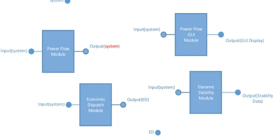
of many modules to be written. Writing the larger program in modules is analogous to the standard engineering black box paradigm. Figure 2.2 illustrates the modularity of the program. Each module of the program can be written, compiled and tested independently
Input(system) Power Flow GUI
Module Output(GUI Display) system Output(system) Power Flow Module Input(system) Output(ED) Economic Dispatch Module Input(system) Input(system) Dynamic Stability Module Output(Stability Data) ED
Figure 2.2: Modularity of the Code. Red Denotes Steady-State Power Flow. Objects are created from classes and modules operate on those classes. Objects which are just instantiation of a class are passed from module to module. This modularity adds great flexibility to the program. Since the power flow data resides in the system object, it is possible for different indi-viduals or entities to design different front ends or graphical user interfaces (GUI) to display the power flow data. It is even possible to re-write this power flow module, with the only requirement being that the interface re-mains the same. It is also possible to incorporate all the modules into one monolithic program; the possibilities are endless.
The code itself is also modular. Type and function declarations are in meaningfully named header (.h) files and function definitions are in mean-ingfully named C++ (.cpp) files. For example, there is a Grid class. The Jacobian class is declared in a grid.h file and is defined in a grid.cpp file. Those files are then included as needed in other files.
2.7
Design Goal – Extensibility
Technologies in electrical engineering change rapidly. Having software that can change as quickly without having to rewrite the entire code base would be a huge benefit. For example, a Nodeclass is created with certain attributes also known in C++ as data members; it also has operations or member functions as they are called in C++.
In power systems, an electrical bus has more information than a basic node. But it also has all the things a basic node has. So the basic node class can be extended to be an electrical bus. Any algorithms that perform operations on a node would then be able to perform those same operations on a bus; e.g., if a function was written to optimally order a set of nodes, that same function would be able to optimally order a set of electrical busses without any change. Extensibility is a powerful feature of the C++ programming language. Figure 2.3 shows this power. Node is the base class for a Bus. A Bus inherits all the attributes and operations of a Node. So, each Bus
has a name, and number, etc. It also inherits functions from theNode
class; functions are often called operations. EachBusname can be obtained by calling the name() operation without parameters or name(newname)
with a string parameter of the newname of the bus.
2.8
Design Goal – Future Computing Technologies
Twenty years ago, many of the technologies in use today were likely not conceivable. It is almost certainly guaranteed that computing technology will continue to evolve. Trending today are Apps, which are used on phones or handheld devices. These devices, such as the Apple iPad Mini, are the most commonly used computing devices by consumers today. Applications are now beginning to move to the cloud. While it is true that in the engineering environment the desktop or workstation is still the most prevalent computing device, it is quite possible this could change. The code produced in this research is written considering that it may someday be ported to a device that fits on a ring on your finger. The code is written to be as generic and as portable as possible; care was taken not to compromise its speed.
class freepower
«struct» Node
+ connectednodes: vector <int> + name: string + number: int «struct» Bus + angle: precisiontype + B: precisiontype + baseMW: precisiontype + G: precisiontype + GenP: precisiontype + GenQ: precisiontype + loadflowarea: int + loadP: precisiontype + loadQ: precisiontype + losszonenumber: int + maxMvarorV: precisiontype + minMvarorV: precisiontype + pqtopv_count: size_t + pvtopq_count: size_t + remotebuscontrolled: int + type: int + vcontrolled: bool + voltage: precisiontype + Vset: precisiontype Figure 2.3: C++ Inheritance
CHAPTER 3
LITERATURE SEARCH
Searching the standard literary sources yielded the paper by Zhou [9] in which he explores the hypothesis that using object oriented programming (OOP) and the C++ language could result in an acceptable power flow program. “Acceptable” means that the resultant program would be small in size and comparable in speed to other solvers written in other languages. Today C++ has proven to be a language of choice when speed or system-level programming is necessary [10]. The debate over the viability C++ and OOP is over; OOP is now proven as the preferred method of programming for purposes. The literature search only entailed looking for projects in which open-source power systems software was written in C++ and had source code available.
There are many IEEE papers that discuss refinement of algorithms, pri-marily Newton-Raphson, to solve the power flow problem. Almost none of them describe implementation of the said algorithm in any specific program-ming language including C++; rather, they give the algorithm in flowchart format. Most papers that give concrete implementations seem to give the implementation as a Matlab program.
During the search, several books were perused, including but not limited to [11], [12], [13], [14]. As programming is just as much style as it is design, the references all had different approaches to the structuring of the software to be written. They had different opinions about what should be classes. While the reading was educational, no specific ideas were taken from any particular source.
CHAPTER 4
SOFTWARE SEARCH
This project is meant to be the beginning of a larger open-source power systems solution solver. The overall vision of the entire package is that it will implement the solvers for the power flow (this work, FreePFlow), opti-mal power flow (OPF), Security Constrained optiopti-mal power flow (SCOPF), dynamic stability and other power systems. A survey of comparable open-source software produced several options, the majority of which were listed on the Task Force on Open-source Software of Power Systems web page [15]. Many of them were written for Matlab; a goal of this work was to provide a standalone package. Complete source code and documentation did not seem to be provided for many of them, as if open-source meant “you can use the software for free.” None were found that were written in C++ and provided full source code for the solution.
While there are commercial software packages that perform the functions of this open-source project, these products are proprietary and do not provide source code; thus, they are not competitors to this project. It is reiterated that this project is provided primarily for academic and research purposes.
CHAPTER 5
SYSTEM FORMAT
To perform power flow analysis of a power system, the system must be de-scribed in some concise manner such that it is easily accessible by some modern computational system. In the early 1970s, such a format was pro-posed and adopted. That data format is known as the IEEE Common Data format (CDF or cdf). The complete specification for this file format can be found in Appendix C.
The program written for this thesis reads system data from a .cdf file [16]. An advantage of using this file format is that there are several IEEE test cases readily available in this format. Disadvantages of this format are its age and that it only stores static data. For this thesis, the CDF format was determined to be sufficient. Figure 5.1 and Figure 5.2 show two formats of a power system. Most humans would prefer the system in the format in Figure 5.1. Computers operate on numbers so Figure 5.2 is preferred when coding; consequently Figure 5.1 must be converted to something like Figure 5.2 in code.
define a power system. This format is more descriptive of a power system, containing such data as synchronous machine and regulator parameters as well as market data just to name a few. This new format is undoubtedly the format of the future, but companies still currently use proprietary formats. This proposed XML format has not been ratified into an IEEE standard. Based on a literature search and a survey of open-source and commercial power systems software, this new XML format has not gained widespread adoption. Should there be no standardization of any particular XML format, future work of this project will use this proposed XML format
01/15/15 MS ARCHIVE 100.
0
1961 W GSO 5 Bus Test Case
BUS DATA FOLLOWS
5 ITEMS 1 One 000 1 1 3 1.000 0. 0 0.0 0.0 0.0 -16.1 100.0 1.000 0.0 0. 0 0.0 0.0 0 2 Two 000 1 1 0 0.0 0.0 800.0 280.0 0.0 0.0 100.0 0.0 0.0 0.0 0.0 0. 0 0 3 Three 000 1 1 2 1.050 0. 0 80.0 40.0 520.0 337.6 100.0 1.050 0.0 0.0 0 .0 0 .0 0 4 Four 000 1 1 0 0.0 0.0 0.0 0.0 0.0 0.0 100.0 0.0 0.0 0.0 0.0 0. 0 0 5 Five 000 1 1 0 0.0 0. 0 0.0 0.0 0.0 0.0 100.0 0.0 0.0 0.0 0.0 0 .0 0 -999
BRANCH DATA FOLLOW
S 5 ITEMS 1 5 1 1 1 0 0.00150 0.02 0 .0 0 0 0 0 0 0.0 0.0 0.0 0.0 0.0 0. 0 0.0 3 4 1 1 1 0 0.00075 0.01 0 .0 0 0 0 0 0 0.0 0.0 0.0 0.0 0.0 0. 0 0.0 4 2 1 1 1 0 0.009 0.1 1 .72 0 0 0 0 0 0.0 0.0 0.0 0.0 0.0 0.0 0.0 5 2 1 1 1 0 0.0045 0.0 5 0.88 0 0 0 0 0 0.0 0.0 0.0 0.0 0 .0 0. 0 0.0 5 4 1 1 1 0 0.00225 0.025 0 .44 0 0 0 0 0 0.0 0.0 0.0 0.0 0.0 0.0 0 .0 -999
LOSS ZONES FOLLOWS
1 ITEMS
1 GSO 30 BUS
-99
INTERCHANGE DATA FOLLOWS
1 ITEMS -9 1 2 Claytor 132 0.0 999.99 GSO
GSO 5 Bus Test Case
TIE LINES FOLLOWS
0 ITEMS
-999
CHAPTER 6
TOOLS
The tools used for this thesis research were:
Intel I7 based computer running Microsoft Windows 8.1 and 10 Microsoft Office 2016
Microsoft Visio 2016
Microsoft Visual Studio 2013 and 2015 Enterprise Edition Git and GitHub
Editor: VIM emulation in Visual Studio Editor: Notepad++ using VIM emulation UML Modeling tool: Astah [18]
UML Modeling tool: Enterprise Architect [19] VIM Notepad++ Adobe Acrobat LATEX Miktek TeXstudio
This code was compiled on an Intel I7 based machine with 8 GB of RAM. The operating system used was Microsoft Windows 10. All code was
writ-The code should be compilable and executable on any x64 machine that has an ISO compliant C++ compiler, with little effort. The final UML models were completed using Enterprise Architect Ultimate by Sparx Systems Pty Ltd. Many of the initial models and concepts were tested using Astah by Astah.net. At the time of the writing of this thesis, Astah provided a free one-year renewable license to the full product. It is easy enough for most coders to code without visualization tools such as UML modelers. UML models make presenting code to others much easier.
CHAPTER 7
USE OF LIBRARIES
There are many libraries that can be used when programming in C++. For matrix manipulations the Matrix Template Library 4 (MTL4) [20] by SimuNova was chosen. The use of this library has many advantages includ-ing reduction in codinclud-ing time. This library has all the support necessary for vector and matrix operations. For example, there is an LU, solver that is used to solve for x givenA and b.
The MTL4 library is large and fairly robust. MTL4 has several different Ax = b solvers but FreePFlow used only the lu solve() solver to imple-ment the Newton-Raphson method. During this project, difficulties were encountered using this library. Using this library, vectors and matrices are not easily inspected in a debugger such as the one in Microsoft Visual Stu-dio. This requires additional steps in the debugging process, such as writing vector elements to other variables for inspection purposes. For this reason, thought was given to writing a matrix library for this project and the creator of C++ was even consulted (see Appendix D); that idea was abandoned for this initial version of the package.
Reasons for choosing C++ include but are not limited to: Object orientation
Modularity Maintainability
Ability to make libraries accessible by other languages Platform portability
CHAPTER 8
OBJECTS
Definitions of the objects used are given below. Objects are capitalized to differentiate them from the physical entities.
Grid – Primarily consists of Branches and Busses. It can contain other devices as necessary.
Branch - Is a connection between Busses.
Bus- Represents an electrical node or bus to which branches, generators, loads, and other devices such as compensators, can be connected.
Generator- Object that models a real-world generator.
Node - Represents a conceptual node as in graph theory. It includes the node’s name, number, the total number of other nodes to which it is connected and a list of other connected nodes. It serves as the base class for a bus.
Note that in C++, structs are classes where all the members and member functions are public. Simple data such as bus and branch data are better represented by structs, thereby eliminating the need to have rudimentary member functions such as getmember() and setmember() to access the data [21]. This thesis may use class for struct, since the original code did im-plement those structs as classes. The released code uses structs for simple data.
CHAPTER 9
CLASSES
In C++, classes are used to encapsulate data along with the functions that operate on that data. Functions in a class are called the member functions. Packaging data along with the functions that operate on the data assists in making code more easily extensible and maintainable. Structs (struct), short for structures, are classes whose members and member functions are all public. This chapter contains a list of the classes and structs used in
FreePFlow.
9.1
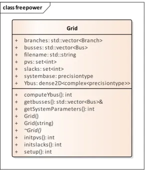
Grid Class
The grid class is a representation of the power grid to be analyzed. The grid is a class that contains private members that are a vector of branches, and vector of buses. Transformer data is contained in the branch data of the .cdf file and subsequently there is not a transformer class.
A parser was written to parse a .cdf file and initialize the branches and nodes of the grid. This parser is a function of the grid class. A graphical representation of this class can be found in Figure 9.1
9.2
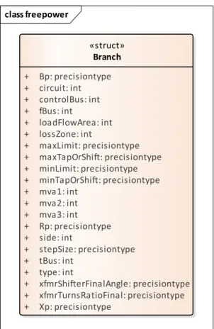
Branch Struct
The branch struct of Figure 9.2 represents a transmission line. Its members hold all the relevant parameters of a transmission line.
class freepower Grid + branches: std::vector<Branch> + busses: std::vector<Bus> + filename: std::string + pvs: set<int> + slacks: set<int> + systembase: precisiontype + Ybus: dense2D<complex<precisiontype>> + computeYbus(): int + getbusses(): std::vector<Bus>& + getSystemParameters(): int + Grid() + Grid(string) + ~Grid() + initpvs(): int + initslacks(): int + setup(): int
Figure 9.1: Grid Class
9.3
Node Struct
The node struct is a class that encapsulates all of the basic attributes of a node. It is the base struct for the bus struct. This struct can be used to write and experiment with code pertaining to graph theory. The node struct is depicted in Figure 9.3.
9.4
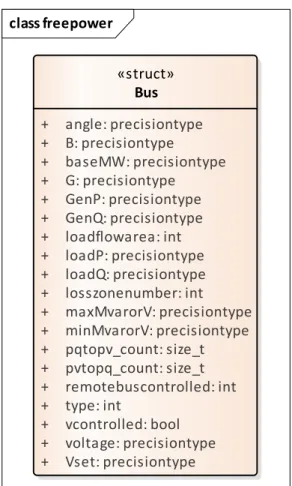
Bus Struct
This Bus struct is a descendant of the Node struct. It extends the Node struct to include all of the attributes specific to an electrical bus in a power grid. It was possible to implement the bus struct fully without creating and implementing the base node struct. Not using inheritance would eliminate using object oriented programming and the Bus struct would have to be implemented completely independent of the Node struct. There would be duplication of some attributes in each struct. The Bus struct is depicted in Figure 9.4.
class freepower «struct» Branch + Bp: precisiontype + circuit: int + controlBus: int + fBus: int + loadFlowArea: int + lossZone: int + maxLimit: precisiontype + maxTapOrShift: precisiontype + minLimit: precisiontype + minTapOrShift: precisiontype + mva1: int + mva2: int + mva3: int + Rp: precisiontype + side: int + stepSize: precisiontype + tBus: int + type: int + xfmrShifterFinalAngle: precisiontype + xfmrTurnsRatioFinal: precisiontype + Xp: precisiontype
Figure 9.2: Branch Struct
9.5
Generator Class
The generator class, Figure 9.5, models a generator. This class is a usable base class that can be extended for different generator types. This class was created for future work in dynamic stability studies; this class is not used in the power flow solution.
9.6
PFSolver Class
The PFSolver Class models a power flow solver. This class takes a Grid object and solves the power flow for that grid. This class does all the work to solve the power flow problem. This class contains member functions that will
class freepower
«struct» Node
+ connectednodes: vector <int> + name: string
+ number: int
Figure 9.3: Node Struct
class freepower «struct» Bus + angle: precisiontype + B: precisiontype + baseMW: precisiontype + G: precisiontype + GenP: precisiontype + GenQ: precisiontype + loadflowarea: int + loadP: precisiontype + loadQ: precisiontype + losszonenumber: int + maxMvarorV: precisiontype + minMvarorV: precisiontype + pqtopv_count: size_t + pvtopq_count: size_t + remotebuscontrolled: int + type: int + vcontrolled: bool + voltage: precisiontype + Vset: precisiontype
class freepower «struct» Generator + angle: precisiontype + Edp: complex<precisiontype> + Efd: complex<precisiontype> + Eqp: complex<precisiontype> + H: precisiontype + Idq: complex<precisiontype> + IGen: complex<precisiontype> + KA: precisiontype + KE: precisiontype + KF: precisiontype + Rf: precisiontype + Rs: precisiontype + SE: complex<precisiontype> + TA: precisiontype + Tdop: precisiontype + TE: precisiontype + TF: precisiontype + TM: complex<precisiontype> + Tqop: precisiontype + Vdq: complex<precisiontype> + VR: complex<precisiontype> + Vref: complex<precisiontype> + Xd: complex<precisiontype> + Xdp: complex<precisiontype> + Xq: complex<precisiontype> + Xqp: complex<precisiontype>
CHAPTER 10
NAMING SCHEME
A consistent naming scheme for variables, user-defined types (UDTs), and functions assist in code readability, maintenance, and debugging. There are several style naming conventions, Hungarian, camelCode, and PascalCode being the most common. The C and C++ languages have their naming con-vention and a derivative of that style is Stroustrup, named after the inventor of the C++ language; Stroustrup is the convention used in this thesis project. C++ Core Guidelines is a new project hosted on GitHub that gives guide-lines on many practices to help C++ programmers to write simpler, more efficient, more maintainable code [21]. Although the code in this project was written prior to the announcement of this project on September 9, 2015, it was edited to adhere as much as possible to those guidelines. Many index variables in loops are suffixed ndx. This adds clarity that the variable is an index and facilitates searching for and modifying it as necessary.
Example
for(size t k=0; k¡N;++k)
becomes
for(size t kndx=0; kndx¡buses.sizeof();++kndx)
Using the above naming scheme trivializes the task of finding and replacing thekndxvariable, in any particular routine, file, or even the entire code base. Beginning coders should try searching for and replacing a variable named n
10.1
Variables
Names of variables were also chosen to match power flow terms; i.e., S is chosen as the variable for complex power. Effort was made to keep names as concise and descriptive as possible while making them unique enough to be easily located using text searches. Vectors, for instance, were suffixed with
vec; e.g.,Svec is the vector of real and reactive powers.
Svec = P1 .. . PN Q1 .. . QN (10.1) where P(δ, V) = S 0 .. . N −1 (10.2) and Q[δ, V] =S N .. . 2N−1 (10.3)
In the code the Jacobian matrix, herein referred to as the Jacobian, is a member of the PFSolver class (see Figure??). The capitalJis unique enough to the code that only it was used for the variable name. The Jacobian is used and defined as follows:
J · " ∆δ ∆V # = " ∆P ∆Q # (10.4) where
J = " ∂P ∂δ ∂P ∂V ∂Q ∂δ ∂Q ∂V # (10.5)
10.2
Functions
Function names use all lower case and are descriptive. Words of functions are separated by an underscore. Global functions are discouraged. All functions are members of a class, and as such, a class must be instantiated to use its function; therefore, functions are very unique. To call a particular function its parent class must be instantiated and then it can be accessed via the call
namespace::classinstance.function name(args) or
namespace::classinstancefunction name(args)
if the object was dynamically allocated. This naming scheme for functions is consistent with [21].
CHAPTER 11
POWER FLOW ALGORITHM
The algorithm used is quite simple. It is very common and based on the classical one proposed by Tinney and Hart [22]. The flowchart in Figure 11.1 shows an overview of the algorithm. The program reads the data of the system from a file, sets up all of the necessary objects, does a Newton-Raphson power flow, and then outputs the results to a text file.
This Power Flow module uses the Newton-Raphson method to solve the Ax=bequation of the power system, whereAis the Jacobian of the system, x is a vector of unknown voltages and angles, and b is the power mismatch. The implementation of this solver is contained in the PFSolver class.
Compute Mismatches Convergence? Solve Aδx=b Convergence? Initialize system Don t forget ε No Output Yes
Yes
Compute Jacobian No Compute YbusCHAPTER 12
CHALLENGES
12.1
Software Design
It is always a challenge to design a complex system. Determining the overall structure and layout of this tool was a daunting task. A wrong decision can lead to unmanageable and non-extensible code. Designing the power flow solver such that it was modular surmounted this challenge. Because the design of the overall power systems analysis tool is a modular one, the
FreePFlow module is only one module of many to be included in the larger
tool. In engineering terms, this modularity is just “black box” design for software. It is challenging to design a very large black box which is composed of many smaller black boxes, particularly when many of the smaller black boxes may change with respect to their input parameters and their output. Thus, much consideration was made in deciding on what classes were to be used.
12.2
Checking Generator Reactive Power Limits
In the real world, generators cannot produce an unlimited amount of reac-tive power; Kundur et al. [23] discuss this topic in detail. A search of the internet for the term “generator capability curve” will also give some insight. The most challenging part of this project was getting the simulated code to converge on all test cases while ensuring that the reactive power limits of the generators were met. Succinctly, in the simulation of the power flow for a system, PV busses are those which have generators attached. Ideally PV busses regulate the voltage on that bus to the voltage set point of the
reaches it upper or lower limit, the PV bus is switched to a PQ bus and the voltage on that PQ bus is set equal to the computed voltage. Checking and enforcing generator reactive power limits can be performed at different times using the Newton-Raphson (N-R) method. Generator reactive power limit checking can be done during each N-R iteration, after the N-R method has converged, or a hybrid of the two. The algorithm used to check and adjust the generator reactive power limits is based on the algorithm found in [24].
12.2.1
During Each N-R Iteration
Theoretically, if the reactive power limits of the generators in the system were checked and corrected after each N-R iteration, then once the N-R method has converged, the result would be a solution to the power flow of that system. The code as it was initially written used this paradigm. After many months of testing and tweaking, it has been determined that this method will not work reliably in all cases, all the time. Testing the code on some cases would work, then tweaking the code to work on other cases would cause it to fail on other cases. In most cases, convergence only was achieved if the checking did not begin until after the first N-R iteration; in other words, in almost all instances if checking reactive power limits on the generators began on the first iteration of the N-R algorithm, the systems diverged.
Much effort was given to making this strategy work, mainly because the strategy described in section 12.2.2 required a major rewrite of the software. After the exhaustive effort to get this paradigm working in the code, the con-clusion was reached that, succinctly, if the changes to the generated reactive power suggested in [24] are performed too early during the N-R iterations, the guess is pushed out of the region of convergence, commonly referred to in the mathematics literature as the basin of attraction. The discussion of this is beyond the scope of this thesis.
12.2.2
After the N-R Method Has Converged
A more reliable method of checking generator reactive power limits is to al-low the N-R algorithm to converge the system (inner loop), be it from a previous solution or a flat start (e.g. δ= 0 and V = 1); check the generator
reactive power limit and adjust them as described by [24] (outer loop); if any adjustment were made in the outer loop, then repeat the inner loop; if no adjustments were made in the outer loop, then the system has converged and the result should be a valid power flow solution with all generator reac-tive power outputs being within each generator’s respecreac-tive lower and upper limits.
This inner/outer loop paradigm is utilized by PowerWorld. To verify the inner loop of FreePFlow, generator reactive power limit was disabled in PowerWorld. The results from FreePFlow’s inner loop matched Power-World’s results within a reasonable tolerance across all the IEEE test cases that were used. Once the outer loop was employed for both, FreePFlow
always converged and provided a valid power flow solution and again the results were close to PowerWorld’s solution; although the solutions were sim-ilar, the variations in the solutions were more significant than when just an inner loop computation was performed. After a discussion with Professor Thomas Overbye, the author became aware than during the power flow cal-culations, at different times during the inner and/or outer loops, PowerWorld uses multipliers to perhaps prevent generators from exceeding reactive power limits, or at least not allow those limits to be exceeded by extreme amounts. With large non-linear systems, there quite possibly are many attractors or solutions to the system, some stable, and some unstable. While it is beyond the scope of this thesis, it is sufficient to mention that it is most probable that PowerWorld’s use of multipliers and other massaging techniques causes PowerWorld to arrive at a valid but slightly different solution from that determined by FreePFlow.
12.2.3
Hybrid
After many hours of writing code and running simulation test cases, it seems conceivable that one could use a hybrid of the two paradigms discussed in sections 12.2.1 and 12.2.2. While it may be possible to devise such a scheme, it is not obvious that there would be any advantages to it over either of the other two ways of checking and correcting generator reactive power limits. Some thought should be put into this idea to be exhaustive; further, Big-O
CHAPTER 13
USE
To use the power flow solver, run the executable from a command line with two parameters. The first parameter is the path and name of the input cdf file. The second parameter is the path and name of the output file. It is recommended that the name of the output file be appended with .txt to denote that it is a text file. Using Microsoft Windows to simulate and the power flow of the IEEE 14 bus example that is in c:\temp, write its results to a text file named ieee14bus-results.txt, open a cmd window and type:
freepflow inputfile outputfile tolerance maxiterations
freepflow c:\temp\ieee14-bus.cdf c:\temp\ieee14bus-results.txt 0.1
10
If tolerance and maxiterations are omitted, the program will run with defaults of 0.1 and 10 respectively for those parameters.
CHAPTER 14
RESULTS
The code works and gives results that are equivalent to those from the educa-tional version of PowerWorld v17, with generator limits disabled and enabled. The output of the power flow is written to an output text file.
The compiled code was tested using the following test cases: Gso5bustest.cdf from [16] ieee14-bus.cdf ieee30-bus.cdf ieee57-bus.cdf ieee118-bus.cdf ieee300-bus.cdf
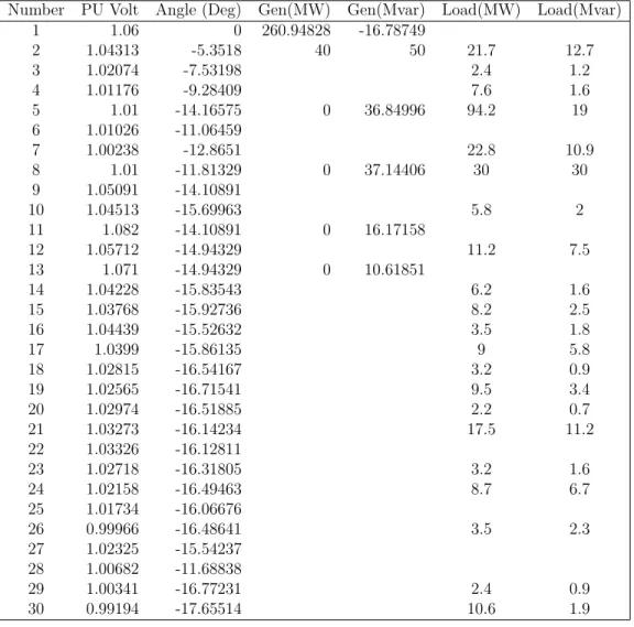
After several months, successful implementation of enforcing the reactive power limits of generators was achieved. The simulation results of the IEEE 30 bus test case from PowerWorld and FreePFlow are shown in Table 14.1 and Table 14.2. There are differences in these results. PowerWorld replaces zero value conductances on line with some very small finite amount. FreeP-Flow does not have a minimum conductance for lines, so that what is speci-fied in the .cdf file is what gets simulated. The MTL4 library also introduces some of this difference.
Table 14.1: PowerWorld IEEE 30 Bus Results
Number PU Volt Angle (Deg) Gen(MW) Gen(Mvar) Load(MW) Load(Mvar)
1 1.06 0 260.94828 -16.78749 2 1.04313 -5.3518 40 50 21.7 12.7 3 1.02074 -7.53198 2.4 1.2 4 1.01176 -9.28409 7.6 1.6 5 1.01 -14.16575 0 36.84996 94.2 19 6 1.01026 -11.06459 7 1.00238 -12.8651 22.8 10.9 8 1.01 -11.81329 0 37.14406 30 30 9 1.05091 -14.10891 10 1.04513 -15.69963 5.8 2 11 1.082 -14.10891 0 16.17158 12 1.05712 -14.94329 11.2 7.5 13 1.071 -14.94329 0 10.61851 14 1.04228 -15.83543 6.2 1.6 15 1.03768 -15.92736 8.2 2.5 16 1.04439 -15.52632 3.5 1.8 17 1.0399 -15.86135 9 5.8 18 1.02815 -16.54167 3.2 0.9 19 1.02565 -16.71541 9.5 3.4 20 1.02974 -16.51885 2.2 0.7 21 1.03273 -16.14234 17.5 11.2 22 1.03326 -16.12811 23 1.02718 -16.31805 3.2 1.6 24 1.02158 -16.49463 8.7 6.7 25 1.01734 -16.06676 26 0.99966 -16.48641 3.5 2.3 27 1.02325 -15.54237 28 1.00682 -11.68838 29 1.00341 -16.77231 2.4 0.9 30 0.99194 -17.65514 10.6 1.9
Table 14.2: PowerWorld IEEE 30 Bus Results
Bus Voltage(V) Angle(deg) GenP(MW) GenQ(MVar) loadP(MW) loadQ(MVar)
1 1.06000 0.00000 260.95189 -16.78737 0.00000 0.00000 2 1.04313 -5.35188 40.00000 50.00000 21.70000 12.70000 3 1.02074 -7.53204 0.00000 0.00000 2.40000 1.20000 4 1.01176 -9.28417 0.00000 0.00000 7.60000 1.60000 5 1.01000 -14.16587 0.00000 36.85033 94.20000 19.00000 6 1.01026 -11.06469 0.00000 0.00000 0.00000 0.00000 7 1.00238 -12.86520 0.00000 0.00000 22.80000 10.90000 8 1.01000 -11.81339 -0.00000 37.14439 30.00000 30.00000 9 1.05091 -14.10900 0.00000 0.00000 0.00000 0.00000 10 1.04513 -15.69972 0.00000 0.00000 5.80000 2.00000 11 1.08200 -14.10900 -0.00000 16.17160 0.00000 0.00000 12 1.05712 -14.94338 0.00000 0.00000 11.20000 7.50000 13 1.07100 -14.94338 0.00000 10.61855 0.00000 0.00000 14 1.04228 -15.83552 0.00000 0.00000 6.20000 1.60000 15 1.03768 -15.92745 0.00000 0.00000 8.20000 2.50000 16 1.04439 -15.52641 0.00000 0.00000 3.50000 1.80000 17 1.03990 -15.86144 0.00000 0.00000 9.00000 5.80000 18 1.02815 -16.54176 0.00000 0.00000 3.20000 0.90000 19 1.02565 -16.71550 0.00000 0.00000 9.50000 3.40000 20 1.02974 -16.51894 0.00000 0.00000 2.20000 0.70000 21 1.03273 -16.14244 0.00000 0.00000 17.50000 11.20000 22 1.03326 -16.12820 0.00000 0.00000 0.00000 0.00000 23 1.02718 -16.31814 0.00000 0.00000 3.20000 1.60000 24 1.02158 -16.49472 0.00000 0.00000 8.70000 6.70000 25 1.01734 -16.06685 0.00000 0.00000 0.00000 0.00000 26 0.99966 -16.48651 0.00000 0.00000 3.50000 2.30000 27 1.02325 -15.54246 0.00000 0.00000 0.00000 0.00000 28 1.00682 -11.68848 0.00000 0.00000 0.00000 0.00000 29 1.00341 -16.77241 0.00000 0.00000 2.40000 0.90000 30 0.99194 -17.65523 0.00000 0.00000 10.60000 1.90000
CHAPTER 15
FUTURE WORK
Some of the work that can be done to improve the power flow module is: Program output should be XML.
Make this solver 3-phase.
Add a GUI to draw a power system.
Possibly add a matrix class - MTL4 is very complex, a simple matrix class may be better.
Simple matrix class - coding of simple LU factorization (lightweight). Introduce CUDA - parallel processing using NVidia graphics processors. Create a cloud or web interface for it.
Optimize the code for particular platforms. Things that can be done with this code are:
Code dynamic stability module.
Code optimal power flow (OPF) model. Code security constrained OPF (SCOPF).
Add features and give back to the GitHub project so that other students can benefit.
CHAPTER 16
CONCLUSION
The outcome of this project is a working power flow module, FreePFlow, that is written in ISO C++14 and is open-source. Complete source code can be obtained from GitHub. It is hoped that this project will be expanded by the community and additions given back to the community. The results given from this FreePFlow match those given by other products. Speed comparisons were not given as many of them rely on the matrix operations involved, and since those were performed by a third-party matrix library [20], it would be more appropriate to gather that information from the provider or owner of that library.
APPENDIX A
THE POWER FLOW PROBLEM
Figure A.1: 3-Bus Simple System
The power flow solution of an electrical power system, often referred to as a grid, is the solution of the steady-state voltages and angles at each bus in the system. Implicit in that solution is the current and power injected and withdrawn from each bus. Figure A.1 is a simple power system with two generators, one load, three busses and two transmission lines. An overview of solving the power flow of a system is given. To solve the power flow problem:
Compute the Ybus for the system
Ybus = Y11 Y12 · · · Y1j Y21 . .. .. . . .. Yi1 Yij (A.1) where Yii= X yii (A.2)
Yij =Yji =− X
yij∀i6= j (A.3)
The diagonal entries of the Ybus are the sum of all admittances
con-nected to the bus.
The Ybus matrix is computed for the convenience of having the
con-ductances and susceptances required for computing the powers in the power flow equations. The conductances (Gs) are the real part of the Ybus entries and the susceptances (Bs) are the imaginary part of the Ybus entries, e.g.,
Yij =Gij +jBij (A.4)
The off-diagonal entries of the Ybus are the negative of the sum of the
admittances connected between buses iand j.
The Ybusin some cases is symmetrical, and when this symmetry occurs
only the diagonal and the upper or lower triangle of it need to be stored. If there are tap or phase changing transformers in the system, theYbus
will not be symmetrical.
Compute the Jacobian for the system
The Jacobian is a gradient of the system. It is a list of sensitivities of real powers to voltages and angles and reactive powers to voltages and angles. The Jacobian of the system is computed by
J = " ∂P ∂δ ∂P ∂V ∂Q ∂δ ∂Q ∂V # (A.5)
The full Jacobian is a 2N square matrix, whereN is the number of busses in the system. The system may be simplified, reducing the size of the Jacobian to less than a 2N ×2N matrix. Details of simplifying the system are given later in this appendix.
The apparent power of each bus is a function of the voltages and an-gles of the bus and all the busses to which it is connected, and the admittances of the lines connected the other busses to it. It is:
Sk=Pk+Qk =Vk N X n Y knVn ej(δk−δn−δkn) (A.6) In rectangular form: Sk =Pk+jQk =Vk N X n=1
YknVn[cos(δk−δn−θkn) +jsin(δk−δn−θkn (A.7)
From A.7 the real and reactive power quantities are obtained by taking the real and imaginary parts of the apparent power, respectively:
Pk= Re{Sk}=Vk N X n=1 YknVncos(δk−δn−θkn) (A.8) Qk= Im{Sk}=Vk N X n=1 YknVnsin(δk−δn−θkn) (A.9) If the norm of the power mismatches is less than a defined tolerance , then the Newton-Raphson iterations can stop; the infinity norm is used.
To solve the power flow, A = J. Initially, the x vector is set to an initial guess of the angles and voltages of the busses of the system. It is initialized as in equation A.10. Don’t forget that J is a function of x. ν denotes the iteration number of the Newton-Raphson method.
xν = " δν Vν # = δν 1 δν 2 .. . δν i V1ν V2ν .. . Vν i (A.10)
The b vector is defined to be the net injected real and reactive powers injected through a path not included in theYbus, andν denotes the iteration
number of the Newton-Raphson method.
bν =S−Sν = " Pν Qν # = P1 −P1ν P2 −P2ν .. . P1 −Piν Q1−Qν1 Q2−Qν2 .. . Qi−Qνi (A.11)
Using A.5, A.10 and A.11 as A, x, and b respectively, the power flow is solved iteratively using the New-Raphson (NR) method. The NR method solves for thexvector by iterating through A.12 and A.13, calculating a new Jacobian during each iteration.
Jxν ∆x= ∆b→J " ∆δ ∆V # = " ∆P ∆Q # (A.12) xν+1 =xν + ∆x (A.13)
We do not invert matrices. The operation is too computationally ex-pensive. Instead we use lower and upper triangular factorization,
for- Simplification – This is important! The A matrix, x and b vectors can be simplified; the entries in them can be removed. The entries corresponding to the slack bus can be removed since the voltage and the angle are known for that bus. Likewise, for generator or PV busses, the voltage is known (it is the desired or set voltage of the generator); thus, the reactive power and voltages entries for the PV busses can be removed from the A matrix, x and b vectors. Figure A.2 and Figure A.3 are the GSO 5-bus test [1] case and the described simplifications. If there are nbusses in a system that has sslack buses andpgenerator (PV) buses, then the Jacobian reduces to a 2n−2s−p squared matrix and the xand b vectors become 2n−2s−p×1 vectors.
APPENDIX B
THE SOLUTION
What constitutes a valid power flow solution of a system? Once a power flow algorithm has solved a system, how does one know if the solution is valid? These questions were posed to others and the answers varied. Based on responses to the above questions, these observations are suggested to determine if a power flow solution may be valid:
1. The algebraic equations used are valid; that is, there are no errors in equations A.1 through A.13.
2. There are no low voltages in the solution.
3. There are no large differences in angles of any bus directly connected to any other bus. The largest difference should be no larger than π 2 radians.
4. The solution must not be an unstable equilibrium point (UEP). Specifics of low and large dare not be given; however, typically, the bus voltages of the system should be close to 1 per unit (pu). And, angle differ-ences between two directly connected busses can only become π
2 radians if the line connecting them is purely inductive. As there is always some resis-tance in a real line, the angle difference between any two directly connected busses should be much less than the limiting π
2 radians.
The fourth item in the list above is not trivial to determine. To determine if the solution is not a UEP, the eigenvalues of the system must be found. For the system to be at a stable equilibrium point (SEP), all of the eigenvalues must lie in the left-hand plane of the imaginary coordinate system. For large systems the computation time may be prohibitive.
Finding a solution to the system Ax = b iteratively is dependent on the initial guess. A wrong guess could cause divergence. Mathematicians use
terms such as attractors, and basins of attraction, in their literature. Af-ter working months on the algorithm that ensures that all generators remain within their reactive power limits, algorithm working, there was an epiphany: When checking generator reactive power limits at each Newton-Raphson it-eration, what if the changes to the generated reactive power on the generator bus were pushing the current guess outside of the region of convergence for the system? That seems to have been the problem! The topic of power flow, Newton-Raphson and basins of attraction, or region of convergence, will be addressed in a later paper. Some details on this issue are provided in [25], [26]. Perhaps the inner/outer loop method described in chapter 12 of this thesis is the best way of using the Newton-Raphson method to achieve a valid power flow solution. It has proven to work on every case on which it was tested. There may be no need to further investigate basins of attraction, etc., with respect to power systems; however, in the spirit of thoroughness, the investigation has already begun. It is important that one understands what constitutes a valid power flow. Searching for written documentation of such proved to be futile. Hopefully, with this section of this thesis, those seeking to learn power flow will have some idea of what they are looking to achieve.
APPENDIX C
CDF FORMAT
Partial Description of the IEEE Common Data Format for the Exchange of Solved Load Flow Data
The complete description can be found in the paper "Common Data Format for the Exchange of Solved Load Flow Data", Working Group on a Common Format for the Exchange of Solved Load Flow Data, \_IEEE Transactions on Power Apparatus and Systems\_, Vol. PAS-92, No. 6, November/December 1973, pp. 1916-1925.
The data file has lines of up to 128 characters. The lines are grouped into sections with section headers. Data items are entered in specific columns. No blank items are allowed, enter zeros instead. Floating point items should have explicit decimal point. No implicit decimal points are used.
Data type codes: A - Alphanumeric (no special characters) I - Integer
F - Floating point * - Mandatory item Title Data
==========
First card in file.
Columns 2- 9 Date, in format DD/MM/YY with leading zeros. If no date
provided, use 0b/0b/0b where b is blank.
Columns 11-30 Originator’s name (A)
Columns 32-37 MVA Base (F*)
Columns 39-42 Year (I)
Column 44 Season (S - Summer, W - Winter)
Bus Data * ==========
Section start card *:
---Columns 1-16 BUS DATA FOLLOWS (not clear that any more than BUS in
1-3 is significant) *
Columns ?- ? NNNNN ITEMS (column not clear, I would not count on this)
Bus data cards *:
---Columns 1- 4 Bus number (I) *
Columns 7-17 Name (A) (left justify) *
Columns 19-20 Load flow area number (I) Don’t use zero! *
Columns 21-23 Loss zone number (I)
Columns 25-26 Type (I) *
0 - Unregulated (load, PQ)
1 - Hold MVAR generation within voltage limits, (PQ) 2 - Hold voltage within VAR limits (gen, PV)
3 - Hold voltage and angle (swing, V-Theta) (must always have one)
Columns 28-33 Final voltage, p.u. (F) *
Columns 34-40 Final angle, degrees (F) *
Columns 41-49 Load MW (F) *
Columns 50-59 Load MVAR (F) *
Columns 60-67 Generation MW (F) *
Columns 68-75 Generation MVAR (F) *
Columns 77-83 Base KV (F)
Columns 85-90 Desired volts (pu) (F) (This is desired remote voltage if
this bus is controlling another bus.
Columns 91-98 Maximum MVAR or voltage limit (F)
Columns 99-106 Minimum MVAR or voltage limit (F)
Columns 107-114 Shunt conductance G (per unit) (F) * Columns 115-122 Shunt susceptance B (per unit) (F) * Columns 124-127 Remote controlled bus number
Section end card:
---Columns 1- 4 -999
Branch Data * =============
Section start card *:
---Columns 40?- ? NNNNN ITEMS (column not clear, I would not count on this) Branch data cards *:
---Columns 1- 4 Tap bus number (I) *
For transformers or phase shifters, the side of the model the non-unity tap is on
Columns 6- 9 Z bus number (I) *
For transformers and phase shifters, the side of the model the device impedance is on.
Columns 11-12 Load flow area (I)
Columns 13-14 Loss zone (I)
Column 17 Circuit (I) * (Use 1 for single lines)
Column 19 Type (I) *
0 - Transmission line 1 - Fixed tap
2 - Variable tap for voltage control (TCUL, LTC) 3 - Variable tap (turns ratio) for MVAR control
4 - Variable phase angle for MW control (phase shifter)
Columns 20-29 Branch resistance R, per unit (F) *
Columns 30-40 Branch reactance X, per unit (F) * No zero impedance lines
Columns 41-50 Line charging B, per unit (F) * (total line charging, +B)
Columns 51-55 Line MVA rating No 1 (I) Left justify!
Columns 57-61 Line MVA rating No 2 (I) Left justify!
Columns 63-67 Line MVA rating No 3 (I) Left justify!
Columns 69-72 Control bus number
Column 74 Side (I)
0 - Controlled bus is one of the terminals 1 - Controlled bus is near the tap side
2 - Controlled bus is near the impedance side (Z bus)
Columns 77-82 Transformer final turns ratio (F)
Columns 84-90 Transformer (phase shifter) final angle (F)
Columns 91-97 Minimum tap or phase shift (F)
Columns 98-104 Maximum tap or phase shift (F)
Columns 106-111 Step size (F)
Columns 113-119 Minimum voltage, MVAR or MW limit (F) Columns 120-126 Maximum voltage, MVAR or MW limit (F) Section end card:
---Columns 1- 4 -999
Loss Zone Data ============== Section start card
is significant)
Columns 40?- ? NNNNN ITEMS (column not clear, I would not count on this)
Loss Zone Cards:
---Columns 1- 3 Loss zone number (I)
Columns 5-16 Loss zone name (A)
Section end card:
---Columns 1- 3 -99
Interchange Data * ================== Section start card
---Columns 1-16 INTERCHANGE DATA FOLLOWS (not clear that any more than
first word is significant).
Columns 40?- ? NNNNN ITEMS (column not clear, I would not count on this)
Interchange Data Cards *:
---Columns 1- 2 Area number (I) no zeros! *
Columns 4- 7 Interchange slack bus number (I) *
Columns 9-20 Alternate swing bus name (A)
Columns 21-28 Area interchange export, MW (F) (+ = out) *
Columns 30-35 Area interchange tolerance, MW (F) *
Columns 38-43 Area code (abbreviated name) (A) *
Columns 46-75 Area name (A)
Section end card:
---Columns 1- 2 -9
Tie Line Data ============= Section start card
---Columns 1-16 TIE LINES FOLLOW (not clear that any more than TIE
Tie Line Cards:
---Columns 1- 4 Metered bus number (I)
Columns 7-8 Metered area number (I)
Columns 11-14 Non-metered bus number (I)
Columns 17-18 Non-metered area number (I)
Column 21 Circuit number
Section end card:
APPENDIX D
CONSULT WITH THE FATHER OF C++
Below is a correspondence with Dr. Bjarne Stroustrup, the inventor of C++, in which he explains why there is not a matrix class in the C++ ISO standard.
On 5/12/2015 11:02 AM, Stevens, Melvin R wrote: Prof./Dr. Stroustrup,
I am coding Power Stability algorithm as an MS/PhD student here at the University of Illinois. I understand that you are a Computer Scientist. From my perspective computer science is a tool used by engineers and scientist to get their work and research done. Linear systems are really at the heart of every scientific, engineering, and mathematic discipline. Matrices are funda-mental to all Linear Systems and are ubiquitous.
Why is there not a C++ Standard Matrix STL? I have read some of your books and kind of understand your philosophy of the C++ Language, but I still see no reason that a true Matrix Library is not a part of the C++ Standard. Currently I am using MTL4 and looked at the Boost class but as each has its own idiosyncrasies and shortcomings, I am thinking of just writing my own which I don’t want to do; I have enough other work to do. The professional wants something very general and complicated and are reluctant to provide simple versions for beginners. Also,
several commercial libraries exist soaking up effort. The
aca-demics are either not interested or only interested in clever nov-elty features.
I am probably 3-4 years away from my PhD. I am hoping that I can use a C++ Standard supplied Matrix Library in my code before then. If you have any video where you discuss this matter, can you please share the urls.
I do what I can (e.g. See the Matrix chapter in TC++PL4)
but for anything to work it would have to come from people using such matrix libraries.
You might like to look at MTL4: http://www.simunova.com/de/node/24 [simunova.com]
Thanks.
I’d also like to thank you for providing Humanity with such a great lan-guage!!!
Thanks.
APPENDIX E
HIDDEN GEMS
In anticipation of having to write a matrix class for FreePFlow, the author preemptively wrote some of the code that would handle the sparsity of power systems. Functions have been written and are contained in the FreePFlow
code that will take as input a grid, which is a form of a graph, and optimally order that grid to minimize matrix operations pertaining to that grid. A description of this process was described by Ogbuobiri et al. [27] and Tinney et al. [28]. Those functions have been thoroughly tested and are known to work.
There are also some routines that pertain to dynamic stability, hence the Generator class in the code. The dynamic stability functions should be moved from this module to a specific module designed for dynamic stability studies. The dynamic stability functions and the Generator class implement an ex-ample found in Power System Dynamics and Stability written by Professors Peter Sauer and M.A. Pai [29].
APPENDIX F
THE CODE
Included below is the complete source code for the project less the copyright and license. Also place GitHub information here.
// FreePFLow.cpp : Defines the entry point for the console application. // #include "stdafx.h" #include <iostream> #include <complex> #include <vector> #include <fstream> #include <algorithm> #include <iterator> #include <string> #include <math.h> #include <cmath> #include"fptypes.h" #include "Grid.h" #include "PFSolver.h" using namespace std; using namespace mtl;
using namespace freepower;
int main(int argc, char* argv[]) {
string inputfile; if (argc > 1) inputfile = argv[1]; else //inputfile = "..\\..\\..\\Data\\GSO5BusTest.cdf"; //inputfile = "..\\..\\..\\Data\\ieee14-bus.cdf"; inputfile = "..\\..\\..\\Data\\ieee30-bus.cdf"; //inputfile = "..\\..\\..\\Data\\ieee57-bus.cdf"; //inputfile = "..\\..\\..\\Data\\ieee118-bus-3.cf"; //inputfile = "..\\..\\..\\Data\\ieee300-bus.cdf"; string outfile; if (argc > 2) outfile = argv[2]; else outfile = "PFSolver_out.txt"; string tol; if (argc > 3) tol = argv[3]; else tol = "1.0E-1";
Grid* testgrid = new Grid(inputfile);
PFSolver pfs(testgrid, outfile, stod(tol.c_str()), 15); int gen_Q_violation{ 1 };
auto outer_iterator{ 0 }; while (gen_Q_violation) {
#if _FULLDEBUG
cout << "Outer Loop Iteration " << outer_iterator << endl; #endif
pfs.NRSolve();
gen_Q_violation = pfs.check_generator_limits(pfs.Svec, pfs. Svec_old, pfs.xvec);
cout << "**** Generator Q Limit Violation: Have to loop again ****" << endl; } #endif outer_iterator++; } delete testgrid; return 0; } #pragma once #include <complex> #include <cmath> #include <fstream> #include <iostream> #include <iomanip> #include <math.h> #include <regex> #include "..\..\libs\boost_1_60_0\boost\numeric\mtl\mtl.hpp" using namespace std; namespace freepower {
typedef double precisiontype;
//Too many digits for precision type but what the heck compiler truncate per platform.
const precisiontype pi =
3.141592653589793238462643383279502884197169399375105 820974944592307816406286208998628034825342117068;
///////////////////////////////////////////////////////////
// Branch struct
// Implementation of the Class Branch
// Original author: Melvin Stevens /////////////////////////////////////////////////////////// struct Branch { precisiontype Bp; int circuit; int controlBus; int fBus; int loadFlowArea; int lossZone; precisiontype maxLimit; precisiontype maxTapOrShift; precisiontype minLimit; precisiontype minTapOrShift; int mva1; int mva2; int mva3; precisiontype Rp; int side; precisiontype stepSize; int tBus; int type; precisiontype xfmrShifterFinalAngle; precisiontype xfmrTurnsRatioFinal; precisiontype Xp; }; /////////////////////////////////////////////////////////// // Node struct
// Implementation of the Class Node
// Created on: 14-Oct-2015 12:16:38 AM
// Original author: Melvin Stevens
/////////////////////////////////////////////////////////// struct Node
//List of connected busses is used to optimally order the graph
vector <int> connectednodes; //List of connected Bus by their indices
};
///////////////////////////////////////////////////////////
// Bus struct
// Implementation of the Class Bus
// Created on: 14-Oct-2015 12:11:10 AM
// Original author: Melvin Stevens
/////////////////////////////////////////////////////////// struct Bus : public Node
{ precisiontype angle; precisiontype B; precisiontype baseMW; precisiontype Vset; precisiontype G; precisiontype GenP; precisiontype GenQ; int loadflowarea; precisiontype loadP; precisiontype loadQ; int losszonenumber; precisiontype maxMvarorV; precisiontype minMvarorV; size_t pvtopq_count; size_t pqtopv_count; int remotebuscontrolled; int type; bool vcontrolled; precisiontype voltage; }; /////////////////////////////////////////////////////////// // Generator struct
// Implementation of the Class Generator
// Created on: 14-Oct-2015 12:16:38 AM
// Original author: Melvin Stevens
/////////////////////////////////////////////////////////// struct Generator
{
precisiontype angle, Rf;
complex<precisiontype> IGen, Idq, Vdq, Edp, Eqp, Efd, VR, Vref, TM;
//Parameters
precisiontype H, Rs, Tdop, Tqop;
complex<precisiontype> Xd, Xdp, Xq, Xqp; //Exciter Paramters
precisiontype KA, TA, KE, TE, KF, TF; complex<precisiontype> SE;
}; }
///////////////////////////////////////////////////////////
// Grid.h
// Implementation of the Class Grid
// Created on: 14-Oct-2015 3:13:46 PM
// Original author: Melvin Stevens
/////////////////////////////////////////////////////////// #if !defined( EA_F88E3EA7_D66D_4b6a_BC4C_CDC0C91B8B59__INCLUDED_) #define EA_F88E3EA7_D66D_4b6a_BC4C_CDC0C91B8B59__INCLUDED_ #include <vector> #include <set> #include <string> #include"fptypes.h" #include "..\..\libs\boost_1_60_0\boost\numeric\mtl\mtl.hpp"
namespace freepower { class Grid { private: //std::vector<Branch> branches; //std::vector<Bus> busses; //std::string filename; //precisiontype systembase; public: std::vector<Branch> branches; std::vector<Bus> busses;
set<int> pvs; //Contains the internal bus number starting with 0.
set<int> slacks;
//vector<int> pvs; //Contains the internal bus number starting with 0. //vector<int> slacks; //set<int> generator_exceeding_limits; std::string filename; precisiontype systembase; dense2D<complex<precisiontype>> Ybus; Grid(); Grid(string in_file_name); virtual ~Grid(); int initpvs(); int initslacks(); int getSystemParameters(); int computeYbus();

![Figure 5.1: Graphical Format of a 5-Bus Power System [1]](https://thumb-us.123doks.com/thumbv2/123dok_us/11023367.2989595/19.918.171.747.731.985/figure-graphical-format-bus-power.webp)