arXiv:1502.07505v1 [stat.ME] 26 Feb 2015
A mixed effect model for bivariate meta-analysis of diagnostic
test accuracy studies using a copula representation of the
random effects distribution
Aristidis K. Nikoloulopoulos∗Abstract
Diagnostic test accuracy studies typically report the number of true positives, false positives, true negatives and false negatives. There usually exists a negative association between the num-ber of true positives and true negatives, because studies that adopt less stringent criterion for declaring a test positive invoke higher sensitivities and lower specificities. A generalized lin-ear mixed model (GLMM) is currently recommended to synthesize diagnostic test accuracy studies. We propose a copula mixed model for bivariate meta-analysis of diagnostic test ac-curacy studies. Our general model includes the GLMM as a special case and can also operate on the original scale of sensitivity and specificity. Summary receiver operating characteristic curves are deduced for the proposed model through quantile regression techniques and differ-ent characterizations of the bivariate random effects distribution. Our general methodology is demonstrated with an extensive simulation study and illustrated by re-analysing the data of two published meta-analyses. Our study suggests that there can be an improvement on GLMM in fit to data and makes the argument for moving to copula random effects models. Our modelling framework is implemented in the packageCopulaREMADAwithin the open source statistical environmentR.
Keywords: copula models; diagnostic tests; multivariate meta-analysis; random effects mod-els; SROC, sensitivity/specificity.
1 Introduction
Synthesis of diagnostic test accuracy studies is the most common medical application of multivariate
meta-analysis [21,30]. Meta-analysis is broadly defined as the quantitative review of the results of
related but independent studies [41]. The purpose of a meta-analysis of diagnostic test accuracy studies is to combine information over different studies, and provide an integrated analysis that will have more statistical power to detect an accurate diagnostic test than an analysis based on a single study. Accurate diagnosis plays an important role in the disease control and prevention [29].
Diagnostic test accuracy studies observe the result of a gold standard procedure which defines the presence or absence of a decease and the result of a diagnostic test. They typically report the number of true positives (diseased people correctly diagnosed), false positives (non-diseased people incorrectly diagnosed as diseased), true negatives and false negatives. As the sensitivity (proportion of those with the disease) and specificity (proportion of those without the disease) are estimated from different samples in each study (diseased and non-diseased patients), they can be assumed to be independent so that the within-study correlations are set to zero [30]. However, there may be a negative between-studies association which should be accounted for. A negative association
∗[email protected], School of Computing Sciences, University of East Anglia, Norwich
between these quantities across studies is likely because studies that adopt less stringent criterion for declaring a test positive invoke higher sensitivities and lower specificities [21].
In situations where studies compare a diagnostic test with its gold standard, heterogeneity arises between studies due to the differences in disease prevalence, study design as well as laboratory and other characteristics [7]. Because of this heterogeneity, a generalized linear mixed model (GLMM)
has been recommended in the biostatistics literature [4,1,14,29] to synthesize information. Note in
passing that it is equivalent with the hierarchical summary receiver operating characteristic model in
Rutter and Gatsonis [46] for the case without covariates [15,5]. The GLMM assumes independent
binomial distributions for the true positives and true negatives, conditional on the latent pair of transformed (via a link function) sensitivity and specificity in each study. The random effects (latent pair of transformed sensitivity and specificity) are jointly analysed with a bivariate normal (BVN) distribution.
Chu et al. [7] propose an alternative mixed model which operates on the original scale of sensitivity and specificity. The random effects follow the bivariate Sarmanov’s [47] family of dis-tributions with beta margins [28]. However, this random effects distribution has a limited range of dependence and is inappropriate for general modelling unless the responses are weakly depen-dent. Hence, this model is too restrictive in the context of diagnostic accuracy studies where strong (negative) dependence is likely.
We propose a copula mixed model as an extension of the GLMM and mixed model in Chu et
al. [7] by rather using a copula representation of the random effects distribution with normal and beta margins, respectively. Copulas are a useful way to model multivariate data as they account for the dependence structure and provide a flexible representation of the multivariate distribution. The theory and application of copulas have become important in finance, insurance and other areas, in order to deal with dependence in the joint tails. Here, we indicate that this can also be important in meta-analysis of diagnostic test accuracy studies. Diagnostic test accuracy studies is a prime area of application for copula models, as the traditional assumption of multivariate normality is invalid in this context.
A copula approach for meta-analysis of diagnostic accuracy studies was recently proposed by Kuss et al. [27] who explored the use of a copula model for observed discrete variables (number of true positives and true negatives) which have beta-binomial margins. This model is actually an approximation of a copula mixed model with beta margins for the latent pair of sensitivity and specificity. Although, this approximation can only be used under the unrealistic case that the number of observations in the respective study group of healthy and diseased probands is the same for each study. In real data applications, the number of true positives and negatives do not have a common support over different studies, hence, one cannot conclude that there is a copula. The natural replicability is in the random effects probability for sensitivity and specificity.
The remainder of the paper proceeds as follows. Section 2 summarizes the standard GLMM
for synthesis of diagnostic test accuracy studies. Section3has a brief overview of relevant copula
theory and then introduces the copula mixed model for diagnostic test accuracy studies and discusses
its relationship with existing mixed models. Section 4 discusses suitable parametric families of
copulas for the copula mixed model, deduces summary receiver operating characteristic curves for the proposed model through quantile regression techniques and different characterizations of the bivariate random effects distribution, and demonstrates that they can show the effect of different
model assumptions. Section5contains small-sample efficiency calculations to investigate the effect
of misspecifying the random effects distribution on parameter estimators and standard errors and
compare the proposed methodology to existing methods. Section 6 summarizes the assessment
of the proposed models using the Vuong’s statistic [53], which is based on sample difference in Kullback-Leibler divergence between two models and can be used to differentiate two parametric
models which could be non-nested. Section7presents applications of our methodology to four data
frames with diagnostic accuracy data from binary test outcomes. We conclude with some discussion
in Section8, followed by a section with the software details and a technical Appendix.
2 The standard GLMM
We first introduce the notation used in this paper. The focus is on two-level (within-study and
for the within study measurements andiis an index for the individual studies. The data, for study
i, can be summarized in a2×2table with the number of true positives (yi1), true negatives (yi2),
false negatives (ni1−yi1), and false positives (ni2−yi2); see Table1.
Table 1: Data from an individual study in a2×2table.
Test Disease (by gold standard)
Yes No
Positive yi1 ni2−yi2 Negative ni1−yi1 yi2
Total ni1 ni2
The standard two-level model of meta-analysing diagnostic test accuracy studies [4,15,1,14,
29] lies in the framework of mixed models [8]. The within-study model assumes that the number
of true positivesYi1and true negativesYi2are conditionally independent and binomially distributed
given X = x, where X = (X1, X2) denotes the bivariate latent (random) pair of transformed
sensitivity and specificity. That is
Yi1|X1=x1 ∼ Binomial ni1, l−1(x1) ; Yi2|X2=x2 ∼ Binomial ni2, l −1 (x2) , (1)
wherel(·)is a link function such as the commonly used logit. The between studies model assumes
thatXis BVN distributed with mean vectorµ = l(π1), l(π2)
⊤
and variance covariance matrix
Σ= σ21 ρσ1σ2 ρσ1σ2 σ22 . That is X∼BVN µ,Σ. (2)
The models in (1) and (2) together specify a GLMM with joint likelihood
L(π1, π2, σ1, σ2, ρ) = N Y i=1 Z Z Y2 j=1 gyij;nij, l−1(xj) φ12(x1, x2;µ,Σ)dx1dx2, where g y;n, π= n y πy(1−π)n−y, y= 0,1, . . . , n, 0< π <1,
is the binomial probability mass function (pmf) and φ12(·;µ,Σ) is the BVN density with mean
vectorµand variance covariance matrixΣ. The parametersπ1 and π2 are those of actual interest
denoting the meta-analytic parameters for the sensitivity and specificity, respectively, while the
univariate parametersσ2
1 andσ22are of secondary interest denoting the variability between studies.
3 The copula mixed model for diagnostic test accuracy studies
In this section, we introduce the copula mixed model for diagnostic test accuracy studies and discuss its relationship with existing mixed models. Before that, the first subsection has some background
on copula models. In Subsection 3.2 and Subsection 3.3 a copula representation of the random
effects distribution with normal and beta margins respectively is presented. We complete this section with details on maximum likelihood estimation.
3.1 Overview and relevant background for copulas
A copula is a multivariate cumulative distribution function (cdf) with uniformU(0,1)margins [22,
33,25]. IfF12 is a bivariate cdf with univariate marginsF1, F2, then Sklar’s [51] theorem implies
that there is a copulaCsuch that
F12(x1, x2) =C
F1(x1), F2(x2)
The copula is unique ifF1, F2 are continuous, but not if some of theFj have discrete components.
IfF12is continuous and(X1, X2)∼F12, then the unique copula is the distribution of(U1, U2) =
(F1(X1), F2(X2))leading to C(u1, u2) =F12 F1−1(u1), F2−1(u2) , 0≤uj ≤1, j = 1,2,
whereFj−1are inverse cdfs. In particular, ifΦ12(·;ρ)is the BVN cdf with correlationρand standard
normal margins, andΦis the univariate standard normal cdf, then the BVN copula is
C(u1, u2) = Φ12 Φ−1 (u1),Φ−1(u2);ρ .
The power of copulas for dependence modelling is due to the dependence structure being considered
separate from the univariate margins; see e.g., [22, Section 1.6]. IfC(·;θ)is a parametric family of
copulas andFj(·;ηj)is a parametric model for thejth univariate margin, then
CF1(x1;η1), F2(x2;η2);θ
is a bivariate parametric model with univariate marginsF1, F2. For copula models, the variables
can be continuous or discrete [38].
3.2 The copula mixed model for the latent pair of transformed sensitivity and specificity
Here we generalize the GLMM by proposing a model that links the two random effects using a copula function rather than the BVN distribution.
The within-study model is the same as in the standard GLMM; see (1). The stochastic represen-tation of the between studies model takes the form
Φ X1;l(π1), σ12 ,Φ X2;l(π2), σ22 ∼C(·;θ), (4)
whereC(·;θ)is a parametric family of copulas with dependence parameterθandΦ(·;µ, σ2)is the
cdf of the N(µ, σ2) distribution. The joint densityf12(x1, x2)of the transformed latent proportions
can be derived as a double partial derivative of the cdf in (3)
f12(x1, x2;π1, π2, σ1, σ2, θ) = ∂CΦ x1;l(π1), σ12 ,Φ x2;l(π2), σ22 ;θ ∂x1∂x2 (5) =cΦ x1;l(π1), σ12 ,Φ x2;l(π2), σ22 ;θφ x1;l(π1), σ21 φ x2;l(π2), σ22 ,
wherec(u1, u2;θ) = ∂2C(u1, u2;θ)/∂u1∂u2 and φ(·;µ, σ2) is the copula and N(µ, σ2) density,
respectively. The models in (1) and (4) together specify a copula mixed model with joint likelihood
L(π1, π2, σ1, σ2, θ) = N Y i=1 Z ∞ −∞ Z ∞ −∞ 2 Y j=1 gyij;nij, l−1(xj) cΦ x1;l(π1), σ21 , (6) Φ x2;l(π2), σ22 ;θ 2 Y j=1 φ xj;l(πj), σj2 dx1dx2 = N Y i=1 Z 1 0 Z 1 0 2 Y j=1 gyij;nij, l−1 Φ−1(uj;l(πj), σ2j) c(u1, u2;θ)du1du2.
It is important to note that the copula parameter θis a parameter of the random effects model
and it is separated from the univariate parameters. The univariate parametersπ1 and π2 are those
of actual interest denoting the meta-analytic parameters for the sensitivity and specificity, while the
univariate parametersσ2
3.2.1 Relationship with the GLMM
In this subsection, we show what happens when the bivariate copula is the BVN copula. The resulting model is the same as the GLMM.
The BVN copula density is
c(u1, u2;ρ) = 1 p 1−ρ2 exp z2 1+z22−2ρz1z2 2p1−ρ2 ! exp z2 1+z22 2 ,
wherezj = Φ−1(uj), j= 1,2. Then foruj = Φ xj;l(πj), σ2j
we havezj = xj−l(πj)
/σj, j=
1,2. Hence, the joint density in (5) becomes
f12(x1, x2;π1, π2, σ1, σ2, ρ) = 1 2πσ1σ2 p 1−ρ2exp h 1 2p1−ρ2 n x1−l(π1)2 2σ12 + x2−l(π2)2 2σ2 2 − 2ρ x1−l(π1) x2−l(π2) σ1σ2 oi ,
which apparently is the BVN densityφ12(x1, x2;µ,Σ).
3.3 The copula mixed model for the latent pair of sensitivity and specificity
The within-study model also assumes that the number of true positivesYi1and true negativesYi2are
conditionally independent and binomially distributed givenX =x, whereX = (X1, X2)denotes
the bivariate latent random pair of sensitivity and specificity. That is
Yi1|X1 =x1 ∼ Binomial(ni1, x1);
Yi2|X2 =x2 ∼ Binomial(ni2, x2). (7)
So one does not have to transform the latent sensitivity and specificity and can work on the original
scale. The Beta(α, β) distribution can be used for the marginal modeling of the latent proportions
and its density is
f(x;α, β) = x α−1
(1−x)β−1
B(α, β) , 0< x <1, α, β >0.
In the sequel we will use the Beta(π, γ) parametrization, whereπ = α+βα (mean parameter) and
γ = α+β+11 (dispersion parameter).
The stochastic representation of the between studies model is
F(X1;π1, γ1), F(X2;π2, γ2)
∼C(·;θ), (8)
whereC(·;θ)is a parametric family of copulas with dependence parameterθand F(·;π, γ)is the
cdf of the the Beta(π, γ) distribution. The models in (7) and (8) together specify a copula mixed
model with joint likelihood
L(π1, π2, γ1, γ2, θ) = N Y i=1 Z 1 0 Z 1 0 2 Y j=1 g(yij;nij, xj)c F(x1;π1, γ1), F(x2;π2, γ2);θ × 2 Y j=1 f(xj;πj, γj)dx1dx2 (9) = N Y i=1 Z 1 0 Z 1 0 2 Y j=1 g yij;nij, F −1 (uj;πj, γj) c(u1, u2;θ)du1du2.
As before, the copula parameterθis a parameter of the random effects model and it is separated
from the univariate parameters, the univariate parametersπ1andπ2are the meta-analytic parameters
3.3.1 Relationship with existing models
Chu et al. [7], instead of using a copula for the random effects distribution or a copula density for
Xin (9), use the Sarmanov’s [47] family of bivariate densities
f12(x1, x2) =f1(x1)f2(x2)
1 +θψ1(x1)ψ2(x2)
,
wherefj(·)is the marginal density ofXj,ψj(·)is a bounded non-constant function such as
R∞ −∞fj(x)
ψj(x)dx= 0, and1 +θψ1(x1)ψ2(x2) ≥0for allx1, x2. For the Sarmanov’s densities if one uses
ψj = 1−2Fj(xj), j = 1,2, then the Farlie–Gumbel–Morgenstern copula (density) is obtained.
However in [7], “kernels” of the typeψj(xj) =xj−E(Xj)are considered as in [28]. The
advan-tage of this choice is that the corresponding likelihood function has a closed form, since the product of integrals can be evaluated analytically. The joint likelihood takes the form
L(π1, π2, γ1, γ2, θ) = N Y i=1 Z 1 0 Z 1 0 2 Y j=1 g(yij;nij, xj)f(xj;πj, γj) 1 +θ 2 Y j=1 xj−πjdx1dx2 = N Y i=1 2 Y j=1 h(yij;nij, πj, γj) 1 +θ 2 Y j=1 yij −nijπj γ−1 j +nij−1 , where h(y;n, π, γ) = n y By+π/γ−π, n−y+ (1−π)(1−γ)/γ Bπ/γ−π,(1−π)(1−γ)/γ , y= 0,1, . . . , n,0< π, γ <1,
is the pmf of a Beta-Binomial(n, π, γ) distribution with meannπand variancenπ(1−π) 1 + (n−
1)γ. The disadvantage of this mixed model is that the Sarmanov’s density with beta margins in [28]
has a limited range of dependence and is inappropriate for general modeling unless the responses are weakly dependent.
Kuss et al. [27] proposed a copula model with beta-binomial margins in this context. This model is actually an approximation of the copula mixed model with beta margins for the latent pair of sensitivity and specificity in (7) and (8). They attempt to approximate the likelihood in (9) with the likelihood of a copula model for observed discrete variables which have beta-binomial margins.
The approximation that they suggest is
L(π1, π2, γ1, γ2, θ)≈ N Y i=1 cH(yi1;ni1, π1, γ1), H(yi2;ni2, π2, γ2);θ Y2 j=1 h(yij;nij, πj, γj),
whereH(·;n, π, γ) is the cdf of the the Beta-Binomial(n, π, γ) distribution. In their
approxima-tion the authors also treat the observed variables which have beta-binomial distribuapproxima-tions as being continuous, and model them under the theory for copula models with continuous margins. Kuss
et al. [27], referring to Genest and Neˇslehov´a [9], claim that there are problems on applying cop-ula to discrete data especially in extreme cases with very small numbers of support points for the discrete marginal distributions. Genest and Neˇslehov´a [9] only warn against estimation for discrete-margined copula models using rank-based methods, instead recommending maximum likelihood estimation. Essentially, Genest et al. [10] apply copula models to multivariate binary data (the ex-treme case of discreteness) and call on composite likelihood techniques for estimation. Multivariate copulas for discrete response data have been in use for a considerable length of time, e.g., in Joe [22], and earlier for some simple copula models. Several examples of copula models for multivari-ate discrete data can be found in the literature; see e.g., [40] for an application in biostatistics and [34] for a survey of copula models and methods for multivariate discrete response data.
However, the main problem in [27] is that the approximation (even if treating the observed variables which have beta-binomial distributions as being discrete) can only be used under the un-realistic case that the number of observations in the respective study group of healthy and diseased
probands nij is the same for each studyi. In real data applications, the discreteYij do not have a
common support over different studies ori, hence, one cannot conclude that there is a copula for
(Yi1, Yi2)that applies when thenij vary with different studiesi. The natural replicability is in the
random effects probability for sensitivity and specificity.
3.4 Maximum likelihood estimation and computational details
Estimation of the model parameters(π1, π2, σ1, σ2, θ)and(π1, π2, γ1, γ2, θ)can be approached by
the standard maximum likelihood (ML) method, by maximizing the logarithm of the joint likelihood in (6) and (9), respectively. The estimated parameters can be obtained by using a quasi-Newton [32] method applied to the logarithm of the joint likelihood. This numerical method requires only the objective function, i.e., the logarithm of the joint likelihood, while the gradients are computed nu-merically and the Hessian matrix of the second order derivatives is updated in each iteration. The standard errors (SE) of the ML estimates can be also obtained via the gradients and the Hessian computed numerically during the maximization process. Assuming that the usual regularity condi-tions [49] for asymptotic maximum likelihood theory hold for the bivariate model as well as for its margins we have that ML estimates are asymptotically normal. Therefore one can build Wald tests to statistically judge any effect.
For mixed models of the form with joint likelihood as in (6) and (9), numerical evaluation of the joint pmf is easily done with the following steps:
1. Calculate Gauss-Legendre quadrature points{uq : q = 1, . . . , nq}and weights {wq : q =
1, . . . , nq}in terms of standard uniform; see e.g., [52].
2. Convert from independent uniform random variables{uq1 :q1= 1, . . . , nq}and{uq2 :q2=
1, . . . , nq}to dependent uniform random variables{uq1 :q1 = 1, . . . , nq}and{C−1(uq2|uq1;θ) :
q1 =q2 = 1, . . . , nq}that have distributionC(·;θ). The inverse of the conditional
distribu-tionC(v|u;θ) =∂C(u, v;θ)/∂ucorresponding to the copulaC(·;θ)is used to achieve this.
3. Numerically evaluate the joint pmf, e.g.,
Z 1 0 Z 1 0 2 Y j=1 g yj;nj, F −1 (uj;πj, γj) c(u1, u2;θ)du1du2 in a double sum: nq X q1=1 nq X q2=1 wq1wq2g y1;n, F −1 (uq1;πj, γj) gy2;n, F −1 C−1(uq2|uq1;θ);πj, γj .
With Gauss-Legendre quadrature, the same nodes and weights are used for different functions; this helps in yielding smooth numerical derivatives for numerical optimization via quasi-Newton
[32]. Our comparisons show that nq = 15 is adequate with good precision to at least at four
decimal places; hence it also provides the advantage of fast implementation.
To sum up, our mixed effect model for meta-analysis of diagnostic test accuracy studies using a copula representation of the random effects distribution with a double integral is straightforward computationally. Note in passing that the linear mixed model in [43] can also provide handy com-putations, but it has limitations due to the use of continuity correction and normal approximation
4 Choices of parametric families of copulas
In our candidate set, families that have different strengths of tail behaviour (see e.g., [17]) are
in-cluded. In the descriptions below, a bivariate copulaCis reflection symmetric if its density satisfies
c(u1, u2) =c(1−u1,1−u2)for all0 ≤u1, u2 ≤1. Otherwise, it is reflection asymmetric often
with more probability in the joint upper tail or joint lower tail. Upper tail dependence means that
c(1−u,1−u) = O(u−1
) asu → 0 and lower tail dependence means that c(u, u) = O(u−1
)
asu → 0. If (U1, U2) ∼ C for a bivariate copula C, then (1 −U1,1−U2) ∼ C180◦, where
C180◦(u1, u2) =u1+u2−1 +C(1−u1,1−u2)is the survival (or rotated by 180 degrees) copula
ofC; this “reflection” of each uniformU(0,1) random variable about1/2changes the direction of
tail asymmetry.
• Reflection symmetric copulas with tail independence satisfyingC(u, u) =O(u2)andC(1−
u,1−u) =O(u2)asu→0, such as the Frank copula with inverse conditional cdf
C−1(v|u;θ) =−1 θlog 1−(1−e−θ ) (v−1 −1)e−θu + 1 , θ∈(−∞,∞)\ {0}.
• Reflection symmetric copulas with intermediate tail dependence [18] such as the BVN copula,
which satisfiesC(u, u, θ) =O(u2/(1+θ)(−logu)−θ/(1+θ)
)asu→0with inverse conditional
cdf
C−1(v|u;θ) = Φp1−ρ2Φ−1
(v) +ρΦ−1(u), θ∈[−1,1].
• Reflection asymmetric copulas with lower tail dependence only such as the Clayton copula
with inverse conditional cdf
C−1 (v|u;θ) =n(v−θ/(1+θ) −1)u−θ + 1o −1/θ , θ∈(0,∞).
• Reflection asymmetric copulas with upper tail dependence only such as the rotated by 180
degrees Clayton copula with inverse conditional cdf
C−1(v|u;θ) = 1−h(1−v)−θ/(1+θ)−1 (1−u)−θ+ 1i
−1/θ
, θ∈(0,∞).
The Frank and BVN copulas interpolate from the Fr´echet lower (perfect negative dependence) to the Fr´echet upper (perfect positive dependence) bound, and, thus they are sufficient from bivariate studies on diagnostic accuracy where negative dependence between the number of true positives and true negatives is expected. The Clayton copula belongs in the Archimedean class of copulas. Archimedean copulas, see e.g. [22], have the form,
C(u1, u2;θ) =φ φ −1 (u1;θ) +φ −1 (u2;θ) ;θ , (10)
where the generatorφ(u;θ)is the Laplace transform (LT) of a univariate family of distributions of
positive random variables indexed by the parameter θ, such thatφ(·) and its inverse have closed
forms. The Clayton copula interpolates from the independence (θ → 0) to the Fr´echet upper
(comonotonic copula) bound (θ→ ∞). For extension of the Laplace transform forθ∈[−1,0), the
Clayton family extends to countermonotonicity (θ→ −1). However this extension is not generally
useful for applications because the support of (10) is not all of (0,1)2 [22, page 109]. Negative
dependence in Clayton copulas can be introduced by applying decreasing transformations to the
“oppositely” ordered variables. If(U1, U2)∼CwhereCis a copula with positive dependence, one
could always get some negative dependence, by supposingC90◦is the copula of(U1,1−U2)
(rota-tion by 90 degrees) orC270◦the copula of(1−U1, U2)(rotation by 270 degrees). So it is worthwhile
to rotate the Clayton copula by 90 and 270 degrees to model negative dependence. These rotated
copulas interpolate from the Fr´echet lower (perfect negative dependence) (θ→ ∞) to the
indepen-dence (θ→0). Negative upper-lower tail dependence means thatc(1−u, u) =O(u−1
)asu →0
and negative lower-upper tail dependence means thatc(u,1−u) = O(u−1
)asu →0[24]. So in
• Reflection asymmetric copula family with negative upper-lower tail dependence, such as the rotated by 90 degrees Clayton copula with inverse conditional cdf
C−1(v|u;θ) =n(vθ/(1−θ)−1)(1−u)θ+ 1o1/θ, θ∈(0,∞).
• Reflection asymmetric copula family with negative lower-upper tail dependence, such as the
as the rotated by 270 degrees Clayton copula with inverse conditional cdf
C−1(v|u;θ) = 1−h(1−v)θ/(1−θ)−1 uθ+ 1i1/θ, θ∈(0,∞).
For this paper, the above copula families are sufficient for the applications in Section 7, since
tail dependence is a property to consider when choosing amongst different families of copulas and the concept of upper/lower tail dependence is one way to differentiate families. Nikoloulopoulos and Karlis [39] have shown that it is hard to choose a copula with similar properties from real data, since copulas with similar (tail) dependence properties provide similar fit. Kuss et al. [27] used, in addition to these copulas, the Placket copula. Plackett copula is a reflection symmetric copula [22, pages 221-22] with tail independence [33, page 215] (not reflection asymmetric copula as stated in [27]) and is not used here since we have included another choice of copulas with similar properties i.e., the Frank copula.
4.1 Summary receiver operating characteristic curves
Rutter and Gatsonis [46] proposed a hierarchical summary receiver operating characteristic (SROC) curve which for some cases is the same with the corresponding GLMM SROC curve [5]. For the GLMM model, the model parameters control the shape of the SROC curve. The GLMM SROC curve can be obtained through a characterization of the estimated bivariate normal distribution by a
line [5,6,7]. Based on the bivariate normality of the random effects, the expected sensitivity for a
chosen specificity in the transformed scale is given in a closed form:
E[X1|X2 =x2] = [l(π1)−ρl(π2)σ1/σ2] +ρl(x2)σ1/σ2. (11)
In general, however,E[X1|X2 =x2]is not in closed form and thus does not have simple expressions
in terms of distribution functions and copulas.
An alternative to the mean for specifying “typical” values of X1 for each value of X2 is the
median, which leads to the notion of median regression ofX1 onX2. Forx2 in range ofX2, let
x1 :=ex1(x2)denote a solution to the equationPr(X1 ≤x1|X2=x2) = 1/2. Then the scatter plot
ofex1(x2)andx2 is the median regression curve ofX1 onX2.
For copula models, median regression curves [33, pages 217–218] can be easily calculated, since Pr(X1 ≤x1|X2 =x2) = Pr U1 ≤F1(x1)|U2=F2(x2) =C(u1|u2) u1=F1(x1) u2=F2(x2) ,
but their shape also depends on the choice of bivariate copulas. Furthermore, as emphasized in [45], since there is no unique definition of a SROC curve, it is preferable and will make more sense to deduce confidence regions as well. To this end in addition of using just median regression curves
we will also exploit the use of quantile regression curves with a focus on high (q = 0.99) and
low quantiles (q = 0.01) which are strongly associated with the upper and lower tail dependence
imposed from each parametric family of copulas. These can be also seen as confidence regions of the median regression SROC curve. Note that Kendall’s tau only accounts for the dependence dominated by the middle of the data, and it is expected to be similar amongst different families
of copulas. However, the tail dependence varies, as explained in Section 4, and is a property to
differentiate amongst different families of copulas. To find the quantile regression curves:
1. SetC(u1|u2;θ) =q.
2. Solve for the quantile regression curveu1:=ue1(u2, q;θ) =C−1(q|u2;θ).
3. For j = 1,2 replace uj by Fj(xj;πj, γj)for beta margins or Φj xj;l(πj), σj for normal
margins.
4. Plotx1:=xe1(x2, q)versusx2.
Of course, the quantile regression curve x2 := ex2(x1, q) ofX2 on X1 is defined similarly.
However, there is no priori reason to regressx1onx2 instead of the other way around [1]. In fact,
if one wants to reserve the nature of a bivariate response instead of a univariate response along with a covariate, then a contour graph can be easily plotted. The contour plot can be seen as the predictive region (analogously to [43]) of the estimated pair of sensitivity and specificity. However, the resulted shape of the prediction region is not depended on the assumption of bivariate normality for the random effects.
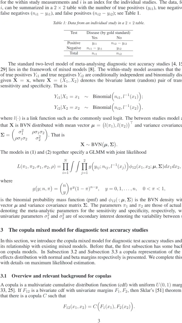
BVN Frank logit(Sensitivity) logit(Specificity) −4 −2 0 2 4 −4 −2 0 2 4 logit(Sensitivity) logit(Specificity) −4 −2 0 2 4 −4 −2 0 2 4 Clayton by 90 Clayton by 270 logit(Sensitivity) logit(Specificity) −4 −2 0 2 4 −4 −2 0 2 4 logit(Sensitivity) logit(Specificity) −4 −2 0 2 4 −4 −2 0 2 4
Figure 1: Contour plots and quantile regression curves from the copula representation of the random effects distribution with normal margins and BVN, Frank, and Clayton by 90 and 270 copulas with the same model parametersπ1 =
0.7, π2 = 0.9, σ1 = 2, σ2 = 1, τ = −0.5 . Red and green lines represent the quantile regression curvesx1 :=
e
x1(x2, q)andx2:=ex2(x1, q), respectively; forq= 0.5solid lines and forq∈ {0.01,0.99}dotted lines.
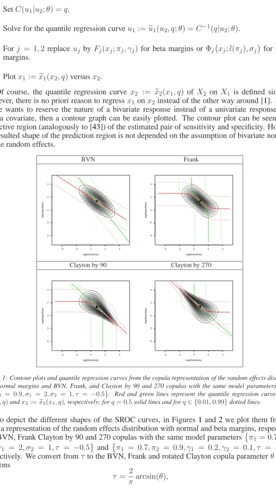
To depict the different shapes of the SROC curves, in Figures 1and 2we plot them from the
copula representation of the random effects distribution with normal and beta margins, respectively,
and BVN, Frank Clayton by 90 and 270 copulas with the same model parametersπ1 = 0.7, π2 =
0.9, σ1 = 2, σ2 = 1, τ = −0.5 and π1 = 0.7, π2 = 0.9, γ1 = 0.2, γ2 = 0.1, τ = −0.5 ,
respectively. We convert fromτ to the BVN, Frank and rotated Clayton copula parameterθvia the
relations
τ = 2
τ = ( 1−4θ−1 −4θ−2R0 θ t et−1dt , θ <0 1−4θ−1 + 4θ−2Rθ 0 et−t1dt , θ >0 , (13) τ = θ/(θ+ 2) , by 0 or 180 degrees −θ/(θ+ 2) , by 90 or 270 degrees (14) in [19], [11], and [12] respectively. BVN Frank Sensitivity Specificity 0.0 0.2 0.4 0.6 0.8 1.0 0.0 0.2 0.4 0.6 0.8 1.0 Sensitivity Specificity 0.0 0.2 0.4 0.6 0.8 1.0 0.0 0.2 0.4 0.6 0.8 1.0 Clayton by 90 Clayton by 270 Sensitivity Specificity 0.0 0.2 0.4 0.6 0.8 1.0 0.0 0.2 0.4 0.6 0.8 1.0 Sensitivity Specificity 0.0 0.2 0.4 0.6 0.8 1.0 0.0 0.2 0.4 0.6 0.8 1.0
Figure 2: Contour plots and quantile regression curves from the copula representation of the random effects distribution with beta margins and BVN, Frank, and Clayton by 90 and 270 copulas with the same model parametersπ1= 0.7, π2=
0.9, γ1= 0.2, γ2= 0.1, τ =−0.5 . Red and green lines represent the quantile regression curvesx1:=xe1(x2, q)and x2:=xe2(x1, q), respectively; forq= 0.5solid lines and forq∈ {0.01,0.99}dotted lines.
5 Small-sample efficiency – Misspecification of the random effects distribution
An extensive simulation study is conducted (a) to gauge the small-sample efficiency of the ML and approximation in Kuss et al. [27]’s (hereafter KHS) methods, and (b) to investigate in detail the misspecification of the parametric margin or family of copulas of the random effects distribution.
To simulate the data we have used the generation process in [42] to get heterogeneous study sizes; the simulation steps follow:
1. Simulate the study sizenfrom a shifted gamma distribution, i.e.,n∼sGamma(α= 1.2, β =
0.01,lag= 30)and round off to the nearest integer.
2. Simulate(u1, u2)from a parametric family of copulasC(;τ);τ is converted to BVN, Frank
and Clayton rotated by 90/270 dependence parameter θ via the relations in (12), (13), and
(14).
3. Convert to beta realizations viaxj =F
−1
j (uj, ∂j, γj)or normal realizations viaxj = Φ
−1
j uj, l(πj), σj
4. Draw the number of diseasedn1from aB(n,0.43)distribution.
5. Setn2=n−n1,yj =njxjand then roundyjforj = 1,2.
We randomly generated B = 104 samples of size N = 20,50 from the Clayton rotated by
270 degrees copula mixed model with beta margins. Table 2 contains the resultant biases, root
mean square errors (RMSE), and standard deviations (SD), along with average theoretical variances
scaled byN, for the MLEs under different copula choices and margins. The theoretical variances
of the MLEs are obtained via the gradients and the Hessian computed numerically during the max-imization process. We also provide biases, RMSEs and SDs for the KHS estimates under the ‘true’ model, i.e., the Clayton rotated by 270 degrees copula mixed model with beta margins.
Conclusions from the values in the table are the following:
• ML with the the ‘true’ copula mixed model is highly efficient according to the simulated
biases and standard deviations.
• The MLEs of the meta-analytic parameters are slightly underestimated under copula
mis-specification. That is, there is some downward bias for these parameters, especially if the “working” model is not close to Kullback-Liebler distance with the “true” model, i.e., it is misspecified. For example in the table there is more bias for the Clayton rotated by 90 de-grees and Frank copulas since they have different tail dependence from the ‘true’ model, i.e., the rotated Clayton by 270 degrees. An interesting result is that the BVN copula performed rather well under misspecification.
• The SDs are rather robust to the copula misspecification.
• The meta-analytic MLEs and SDs are not robust to the margin misspecification, while the
MLE ofτ and its SD is.
• The KHS approximation method yields to biased univariate parameter estimates.
• The efficiency of the KHS approximation method is low for the dependence parameterτ. The
parameterτ is substantially underestimated.
The simulation results indicate that the KHS approximation method in [27] is an inefficient; hence flawed method. This was expected, since theoretically there are serious problems on mod-elling assumptions under the case of heterogeneous study sizes. If the number of true positives and negatives do not have a common support over different studies, then one cannot conclude that there is a copula. To make our study complete, we perform theoretical calculations, similarly to
[23,35,37], to investigate the accuracy of the approximate copula likelihood method in [27] for
the special case of a constant sizenof groups of diseased and healthy people in the single studies
and show whether or not this leads to consistent estimate of the parameters of the bivariate random effects distribution. As shown in the Appendix, the KHS method leads to asymptotic bias for both the univariate and copula parameters and hence there is no consistency. Also given the resultant substantial asymptotic downward bias for the dependence parameter, the approximation deterio-rates, and, hence cannot be used e.g., for prediction purposes via SROC curves. To this end, the KHS approximation method is not used in the sequel, since its inefficiency has been shown, and, it should be avoided for bivariate meta-analysis of diagnostic test accuracy studies.
The effect of misspecifying the copula choice can be seen as minimal for both the univariate parameters and Kendall’s tau. However, note that (a) the meta-analytic parameters are a univariate inference, and hence it is the univariate marginal distribution that matters and not the type of the copula, and, (b) as previously emphasized Kendall’s tau only accounts for the dependence dom-inated by the middle of the data (sensitivities and specificities), and it is expected to be similar amongst different families of copulas. However, the tail dependence varies, as explained in Section 4, and is a property to consider when choosing amongst different families of copulas, and, hence affects the shape of SROC curves, i.e., prediction. SROC will essentially show the effect of different model (random effect distribution) assumptions, since it is an inference that depends on the joint distribution.
Table 2: Small sample of sizesN = 20,50simulations (104replications) from the Clayton rotated by 270 degrees copula mixed model with beta margins and resultant biases, root mean
square errors (RMSE) and standard deviations (SD), along with the square root of the average theoretical variances (√V¯), scaled byN, for the MLEs under different copula choices and
margins. We also provide biases, RMSEs and SDs for the KHS estimates under the ‘true’ model.
Margin Copula π1= 0.7 π2= 0.9 γ1= 0.2 γ2= 0.1 τ=−0.5 N= 20 N = 50 N = 20 N= 50 N= 20 N = 50 N= 20 N= 50 N = 20 N= 50 NBias Beta BVN -0.02 -0.09 0.00 -0.06 -0.64 -1.24 -0.32 -0.51 -1.54 -2.31 Frank -0.23 -0.72 0.10 0.27 -0.59 -1.08 -0.39 -0.72 -2.01 -3.77 Clayton by 90 -0.11 -0.31 -0.02 -0.13 -0.50 -0.81 -0.20 -0.14 -0.23 2.74 Clayton by 270 -0.01 -0.08 0.03 0.04 -0.65 -1.25 -0.40 -0.78 -2.30 -4.57 Normal BVN 0.71 1.87 0.63 1.64 - - - - -1.56 -2.26 Frank 0.46 1.11 0.68 1.79 - - - - -1.95 -3.52 Clayton by 90 0.62 1.65 0.64 1.67 - - - - -0.25 2.66 Clayton by 270 0.70 1.89 0.62 1.62 - - - - -2.39 -4.69 KHS Clayton by 270 1.99 5.58 -0.26 -0.55 -0.48 -1.01 -1.44 -3.87 7.42 20.09 NSD Beta BVN 0.94 1.47 0.44 0.72 1.01 1.63 0.71 1.22 3.31 4.83 Frank 1.00 1.58 0.42 0.68 1.01 1.62 0.67 1.13 3.36 4.84 Clayton by 90 0.97 1.50 0.46 0.78 1.10 1.80 0.87 1.52 4.83 7.15 Clayton by 270 0.94 1.47 0.43 0.70 0.97 1.56 0.64 1.07 3.12 4.54 Normal BVN 1.06 1.66 0.38 0.59 4.77 7.35 5.02 7.93 3.35 4.76 Frank 1.11 1.76 0.38 0.59 4.70 7.24 5.04 7.99 3.40 4.92 Clayton by 90 1.11 1.72 0.38 0.60 5.19 8.13 5.52 8.88 4.76 6.74 Clayton by 270 1.06 1.66 0.38 0.59 4.52 6.86 4.97 7.77 3.18 4.62 KHS Clayton by 270 1.17 1.95 0.56 0.77 1.04 1.68 0.76 0.72 1.82 1.48 N√V¯ Beta BVN 0.76 1.25 0.40 0.66 0.79 1.29 0.61 1.02 2.67 3.86 Frank 0.77 1.27 0.37 0.59 0.82 1.33 0.58 0.95 2.62 3.78 Clayton by 90 0.77 1.25 0.39 0.65 0.83 1.34 0.64 1.10 3.00 4.11 Clayton by 270 0.75 1.22 0.38 0.60 0.77 1.25 0.56 0.90 2.56 3.72 Normal BVN 0.87 1.45 0.32 0.53 3.70 5.82 4.58 7.35 2.90 3.84 Frank 0.87 1.45 0.31 0.50 3.74 5.92 4.58 7.31 2.56 3.69 Clayton by 90 0.89 1.48 0.33 0.54 3.87 6.15 4.57 7.44 2.90 3.94 Clayton by 270 0.84 1.36 0.31 0.49 3.52 5.47 4.46 6.96 2.45 3.48 NRMSE Beta BVN 0.94 1.47 0.44 0.72 1.19 2.05 0.78 1.32 3.65 5.35 Frank 1.02 1.74 0.43 0.73 1.17 1.95 0.77 1.34 3.92 6.13 Clayton by 90 0.97 1.53 0.46 0.80 1.21 1.97 0.89 1.53 4.84 7.65 Clayton by 270 0.94 1.47 0.43 0.70 1.17 2.00 0.75 1.33 3.87 6.44 Normal BVN 1.27 2.50 0.74 1.74 - - - - 3.69 5.27 Frank 1.20 2.08 0.78 1.88 - - - - 3.92 6.05 Clayton by 90 1.27 2.39 0.75 1.77 - - - - 4.77 7.24 Clayton by 270 1.27 2.52 0.73 1.73 - - - - 3.98 6.58 KHS Clayton by 270 2.31 5.91 0.62 0.94 1.15 1.96 1.63 3.93 7.64 20.14 1 3
6 Vuong’s test for model comparison
In this section we provide a methodology for the comparison of non-nested models. It would be used as a tool to show if the copula mixed model provides better fit than the standard GLMM. We will call a test proposed by Vuong [53]. The Vuong’s test is the sample version of the difference in Kullback-Leibler divergence between two models and can be used to differentiate two parametric models which could be non-nested.This test has been used extensively in the copula literature to
compare copula models, see e.g., [2,3,25]
Assume that we have Models 1 and 2 with parametric densities f(1)andf(2)respectively. We
can compare ∆1fz =N −1hX i {Efz[logf z (Y1, Y2)]−Efz[logf(1)(Y1, Y2;θ(1))]} i , and ∆2fz =N −1hX i {Efz[logf z (Y1, Y2)]−Efz[logf(2)(Y1, Y2;θ(2))]} i ,
whereθ(1),θ(2)are the parameters in Models 1 and 2 respectively that lead to the closest
Kullback-Leibler divergence to the truefz
; equivalently they are the limits in probability of the MLEs based
on models 1 and 2 respectively. Model 1 is closer to the truefz
, i.e., is the better fitting model if
∆ = ∆1fz−∆2fz <0, and Model 2 is the better fitting model if∆>0. The sample version of
∆with MLEsθˆ(1),θˆ(2)is ¯ D= N X i=1 Di/N, whereDi = log " f(2) Y1,Y2;ˆθ(2) f(1)Y1,Y2;ˆθ(1) #
. Vuong [53] has shown that asymptotically
√ ND/s¯ ∼N(0,1), wheres2= N1−1 PN i=1(Di−D¯)2. 7 Illustrations
We illustrate the use of the copula mixed model by re-analysing the data of two published
meta-analysis [48,13]. These data have been frequently used as an example for methodological papers
on meta-analysis of diagnostic accuracy studies [43,4,46,44,16,27].
We fit the copula mixed model for all different choices of parametric families of copulas and margins. To make it easier to compare strengths of dependence, we convert the copula parameters to
Kendall’sτ’s via the relations in (12), (13), and (14) for BVN, Frank and rotated Clayton copulas,
respectively. Since the number of parameters is the same between the models, we use the log-likelihood at estimates as a rough diagnostic measure for goodness of fit between the models. We further compute the Vuong’s tests with Model 1 being the BVN copula mixed model with normal margins, i.e., the standard GLMM, to reveal if any other copula mixed model provides better fit than the standard GLMM.
Finally, we demonstrate SROC curves and summary operating points (a pair of average
sensi-tivity and specificity) with a confidence region and a predictive region as deduced in Section4.1.
7.1 The telomerase and computed tomography data
In Glas et al. [13] the telomerase marker for the diagnosis of bladder cancer is evaluated using 10 studies. The size in each study ranges from 35 to 195. The interest was to define if this non-invasive and cheap marker could replace the standard of cystoscopy or histopathology. Riley et al. [44]
applied the GLMM with different starting values and all produced a between-study correlation
esti-mate of−1but with different meta-analytic parameter point estimates and standard errors. Clearly
at this example, it is not possible to estimate the correlation between the logit sensitivity and speci-ficity, and the maximum likelihood estimator should truncate the correlation to the left boundary of
its parameter space, i.e.,−1. In [27] it is acknowledged that the copula model for observed discrete
variables which have beta-binomial margins yields sensible estimates for the dependence parameter and its standard error. This result is in error and due to the fact that the KHS method underestimates
the dependence parameter as emphasized in Section5and shown in the Appendix forρ=−1.
Fitting the copula mixed model for all different choices of parametric families of copulas and margins, the resultant estimate of the dependence parameter was close to the boundary of its param-eter space. If the dependence paramparam-eter estimate is so large (on absolute value), the copula should be set to countermonotonic (Fr´echet lower bound), and, then optimize over the remaining (univari-ate) parameters. With other words there exists negative perfect dependence, and thus there is only one copula: the countermonotonic copula. This is a limiting case for all the parametric families
of copulas, listed in Section4, when the dependence parameter is fixed to the left boundary of its
parameter space.
This was also the case for the analysis of the data on 17 studies of computed tomography (CT) for the diagnosis of lymph node metastasis in women with cervical cancer, one of three imaging techniques in the meta-analysis in [48]. The size in each study ranges from 20 to 253. Diagnosis of metastatic disease by CT relies on nodal enlargement.
Table 3: Maximised log-likelihoods, estimates and standard errors (SE), along with the Vuong’s statistics andp-values for the telomerase and computed tomography data.
Telomerase Computed Tomography
Normal margins Beta margins Normal margins Beta margins
Est. SE Est. SE Est. SE Est. SE
π1 0.77 0.03 π1 0.76 0.03 π1 0.46 0.07 π1 0.46 0.06 π2 0.91 0.05 π2 0.81 0.06 π2 0.93 0.01 π2 0.92 0.01 σ1 0.43 0.13 γ1 0.03 0.02 σ1 1.00 0.27 γ1 0.17 0.07 σ2 1.83 0.40 γ2 0.28 0.10 σ2 0.60 0.23 γ2 0.02 0.02
logL -50.37 logL -51.14 logL -69.37 logL -69.58
Vuong’s test Vuong’s test
√
ND/s¯ - √ND/s¯ -1.580 - -1.416
p-value - p-value 0.114 - 0.157
Table3gives the estimated univariate parameters, standard errors, and log-likelihoods for both
normal and beta margins for both datasets. For telomerase data, both models agree on the
esti-mated sensitivity πˆ1 but the estimate of specificity πˆ2 is larger under the standard GLMM. The
log-likelihood is−50.37for normal margins and−51.14for beta margins, and thus a normal
mar-gin seems to be a better fit for the data. Furthermore, according to the Vuong’s test the copula
mixed model with normal margins (i.e., the standard GLMM) provides marginally better fit (p
-value= 0.114). For computed tomography data, both models agree on the estimated sensitivity ˆπ1
and specificityˆπ2. The log-likelihood is−69.37for normal margins and−69.58for beta margins,
and thus a normal margin seems to be a better fit for the data. However, according to the Vuong’s test the copula mixed model with normal margins (i.e., the standard GLMM) does not provide statistical
significant better fit (p-value= 0.157).
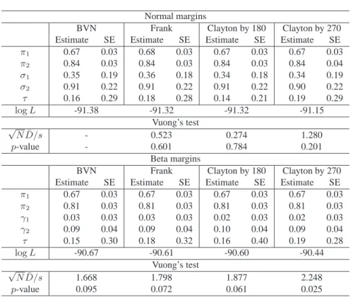
Finally, figure3 also shows the SROC curves for both datasets and the visual fit is consistent
with the model fitting and comparison in Table3. Note in passing since we are dealing with the
countermonotonic copula all the quantile regression curves almost coincide, and hence we just depict one median regression curve for each model.
Telomerase Computed Tomography 0.0 0.2 0.4 0.6 0.8 1.0 0.0 0.2 0.4 0.6 0.8 1.0 Sensitivity Specificity Normal Beta 0.0 0.2 0.4 0.6 0.8 1.0 0.0 0.2 0.4 0.6 0.8 1.0 Sensitivity Specificity Normal Beta
Figure 3: SROC curves from the countermonotonic copula representation of the random effects distribution with normal margins (black line) and beta (red line) margins for the telomerase and computed tomography data.
7.2 The lymphangiography data
In this section we apply the copula mixed models to data on 17 studies of lymphangiography for the diagnosis of lymph node metastasis in women with cervical cancer, one of three imaging techniques in the meta-analysis in [48]. The size in each study ranges from 21 to 300. Diagnosis of metastatic disease by lymphangiography is based on the presence of nodal-filling defects.
Table 4: Maximised log-likelihoods, estimates and standard errors (SE), along with the Vuong’s statistics andp-values for the lymphangiography data.
Normal margins
BVN Frank Clayton by 180 Clayton by 270
Estimate SE Estimate SE Estimate SE Estimate SE
π1 0.67 0.03 0.68 0.03 0.67 0.03 0.67 0.03 π2 0.84 0.03 0.84 0.03 0.84 0.03 0.84 0.04 σ1 0.35 0.19 0.36 0.18 0.34 0.18 0.34 0.19 σ2 0.91 0.22 0.91 0.22 0.91 0.22 0.90 0.22 τ 0.16 0.29 0.18 0.28 0.14 0.21 0.19 0.29 logL -91.38 -91.32 -91.32 -91.15 Vuong’s test √ ND/s¯ - 0.523 0.274 1.280 p-value - 0.601 0.784 0.201 Beta margins
BVN Frank Clayton by 180 Clayton by 270
Estimate SE Estimate SE Estimate SE Estimate SE
π1 0.67 0.03 0.67 0.03 0.67 0.03 0.67 0.03 π2 0.81 0.03 0.81 0.03 0.81 0.03 0.81 0.03 γ1 0.03 0.03 0.03 0.03 0.02 0.03 0.02 0.03 γ2 0.09 0.04 0.09 0.04 0.10 0.04 0.09 0.04 τ 0.15 0.30 0.18 0.32 0.16 0.40 0.19 0.28 logL -90.67 -90.61 -90.60 -90.44 Vuong’s test √ ND/s¯ 1.668 1.798 1.877 2.248 p-value 0.095 0.072 0.061 0.025
In Table4we report the resulting maximized log-likelihoods, estimates, and standard errors of
the copula mixed models with different choices of parametric families of copulas and margins. All
models agree on the estimated sensitivityπˆ1, but the estimateˆπ2of specificity is smaller when beta
margins are assumed. The log-likelihoods show that a copula mixed model with rotated by 270 degrees Clayton copula and beta margins provides the best fit. It is revealed that a copula mixed model with the sensitivity and specificity on the original scale provides better fit than the GLMM, which models the sensitivity and specificity on a transformed scale. The improvement over the
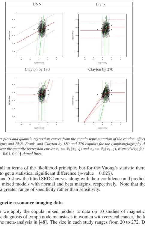
BVN Frank logit(Sensitivity) logit(Specificity) −4 −2 0 2 4 −4 −2 0 2 4 logit(Sensitivity) logit(Specificity) −4 −2 0 2 4 −4 −2 0 2 4 Clayton by 180 Clayton by 270 logit(Sensitivity) logit(Specificity) −4 −2 0 2 4 −4 −2 0 2 4 logit(Sensitivity) logit(Specificity) −4 −2 0 2 4 −4 −2 0 2 4
Figure 4: Contour plots and quantile regression curves from the copula representation of the random effects distribution with normal margins and BVN, Frank, and Clayton by 180 and 270 copulas for the lymphangiography data. Red and green lines represent the quantile regression curvesx1:=ex1(x2, q)andx2:=ex2(x1, q), respectively; forq= 0.5solid
lines and forq∈ {0.01,0.99}dotted lines.
GLMM is small in terms of the likelihood principle, but for the Vuong’s statistic there is enough
improvement to get a statistical significant difference (p-value= 0.025).
Figures4and5show the fitted SROC curves along with their confidence and prediction regions
for the copula mixed models with normal and beta margins, respectively. Note that the predictive regions cover a greater range of specificity rather than sensitivity.
7.3 The magnetic resonance imaging data
In this section we apply the copula mixed models to data on 10 studies of magnetic resonance imaging for the diagnosis of lymph node metastasis in women with cervical cancer, the last imaging technique in the meta-analysis in [48]. The size in each study ranges from 20 to 272. Diagnosis of metastatic disease by lymphangiography relies on nodal enlargement.
In Table5we report the resulting maximized log-likelihoods, estimates, and standard errors of
the copula mixed models with different choices of parametric families of copulas and margins. All
models roughly agree on the estimated sensitivityπˆ1and specificityπˆ2, but both are slightly smaller
when beta margins are assumed. The log-likelihoods show that a rotated by 270 degrees Clayton copula mixed model with normal or beta margins provides the best fit. Although, the rotated by 270 degrees Clayton copula mixed model provides better fit than the GLMM, the difference, according
to Vuong’s test, is not statistical significant (p-value=0.156).
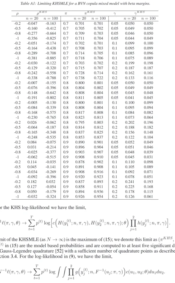
Figures6and7show the fitted SROC curves along with their confidence and prediction regions
for the copula mixed models with normal and beta margins, respectively. Note that the predictive regions cover a greater range of sensitivity rather than specificity.
BVN Frank Sensitivity Specificity 0.0 0.2 0.4 0.6 0.8 1.0 0.0 0.2 0.4 0.6 0.8 1.0 Sensitivity Specificity 0.0 0.2 0.4 0.6 0.8 1.0 0.0 0.2 0.4 0.6 0.8 1.0 Clayton by 180 Clayton by 270 Sensitivity Specificity 0.0 0.2 0.4 0.6 0.8 1.0 0.0 0.2 0.4 0.6 0.8 1.0 Sensitivity Specificity 0.0 0.2 0.4 0.6 0.8 1.0 0.0 0.2 0.4 0.6 0.8 1.0
Figure 5: Contour plots and quantile regression curves from the copula representation of the random effects distribution with beta margins and BVN, Frank, and Clayton by 180 and 270 copulas for the lymphangiography data. Red and green lines represent the quantile regression curvesx1:=ex1(x2, q)andx2:=ex2(x1, q), respectively; forq= 0.5solid lines
and forq∈ {0.01,0.99}dotted lines.
Table 5: Maximised log-likelihoods, estimates and standard errors (SE), along with the Vuong’s statistics andp-values for the magnetic resonance imaging data.
Normal margins
BVN Frank Clayton by 90 Clayton by 270
Estimate SE Estimate SE Estimate SE Estimate SE
π1 0.55 0.11 0.54 0.10 0.54 0.11 0.55 0.10 π2 0.95 0.02 0.96 0.02 0.95 0.02 0.96 0.02 σ1 1.16 0.39 1.14 0.38 1.21 0.41 1.13 0.37 σ2 0.87 0.34 0.83 0.32 0.85 0.34 0.87 0.32 τ -0.51 0.29 -0.47 0.28 -0.48 0.33 -0.49 0.26 logL -46.26 -46.35 -46.72 -45.90 Vuong’s test √ ND/s¯ - -0.815 -2.175 1.419 p-value - 0.415 0.030 0.156 Beta margins
BVN Frank Clayton by 90 Clayton by 270
Estimate SE Estimate SE Estimate SE Estimate SE
π1 0.54 0.08 0.53 0.08 0.53 0.08 0.54 0.08 π2 0.94 0.02 0.94 0.02 0.94 0.02 0.94 0.02 γ1 0.21 0.10 0.21 0.10 0.22 0.10 0.21 0.09 γ2 0.04 0.03 0.03 0.02 0.03 0.03 0.04 0.02 τ -0.53 0.28 -0.47 0.28 -0.50 0.33 -0.50 0.25 logL -46.27 -46.39 -46.75 -45.86 Vuong’s test √ ND/s¯ -0.014 -0.422 -1.326 0.935 p-value 0.989 0.673 0.185 0.350
BVN Frank logit(Sensitivity) logit(Specificity) −4 −2 0 2 4 −4 −2 0 2 4 logit(Sensitivity) logit(Specificity) −4 −2 0 2 4 −4 −2 0 2 4 Clayton by 90 Clayton by 270 logit(Sensitivity) logit(Specificity) −4 −2 0 2 4 −4 −2 0 2 4 logit(Sensitivity) logit(Specificity) −4 −2 0 2 4 −4 −2 0 2 4
Figure 6: Contour plots and quantile regression curves from the copula representation of the random effects distribution with normal margins and BVN, Frank, and Clayton by 90 and 270 copulas for the magnetic resonance imaging data. Red and green lines represent the quantile regression curvesx1:=xe1(x2, q)andx2:=ex2(x1, q), respectively; forq= 0.5
solid lines and forq∈ {0.01,0.99}dotted lines.
8 Discussion
We have proposed a copula mixed model for bivariate meta-analysis of diagnostic test accuracy studies. This is the most general meta-analytic model, with univariate parameters separated from dependence parameters. Our general model includes the GLMM as a special case and can provide an improvement over the latter based on log-likelihood and Vuong’s [53] statistic, and thus can provide a better statistical inference for the SROC. This improvement relies on the fact that the random effects distribution is expressed via copulas which allow for flexible dependence modelling, different from assuming simple linear correlation structures, normality and tail independence, which makes them well suited to the aforementioned application area.
Building on the basic model proposed in this paper, there are several extensions that can be implemented. The copula mixed model can also easily be extended in any context where clinical trials or observational studies report more than a single outcome and to inclusion of covariates. However, larger sample sizes will be required to estimate the effect of covariates in bivariate meta-regression, where the underlying treatment effects depend on covariates. This is typical in the univariate meta-regression [20].
Another direction of future research is to extend our copula-based meta-analytic model to the
d-variate (d > 2) case. There are many simple bivariate copula families, but generally their
mul-tivariate extensions have limited dependence structures. However, in recent years, a popular and
useful approach is the vine pair-copula construction, see e.g., [26,25], which is based ond(d−1)/2
bivariate copulas. Some studies also may not report alldoutcomes. In such cases our model can be
extended for missing data via pattern mixture models. Pattern mixture models are studied in [50] for copulas and in [31] for pairwise and network meta-analysis.
BVN Frank Sensitivity Specificity 0.0 0.2 0.4 0.6 0.8 1.0 0.0 0.2 0.4 0.6 0.8 1.0 Sensitivity Specificity 0.0 0.2 0.4 0.6 0.8 1.0 0.0 0.2 0.4 0.6 0.8 1.0 Clayton by 90 Clayton by 270 Sensitivity Specificity 0.0 0.2 0.4 0.6 0.8 1.0 0.0 0.2 0.4 0.6 0.8 1.0 Sensitivity Specificity 0.0 0.2 0.4 0.6 0.8 1.0 0.0 0.2 0.4 0.6 0.8 1.0
Figure 7: Contour plots and quantile regression curves from the copula representation of the random effects distribution with beta margins and BVN, Frank, and Clayton by 90 and 270 copulas for the magnetic resonance imaging data. Red and green lines represent the quantile regression curvesx1:=xe1(x2, q)andx2:=ex2(x1, q), respectively; forq= 0.5
solid lines and forq∈ {0.01,0.99}dotted lines.
Software
A contributedRpackageCopulaREMADA[36] has functions to implement the copula mixed model
for meta-analysis of diagnostic test accuracy studies and produce SROC curves and summary oper-ating points (a pair of average sensitivity and specificity) with a confidence region and a predictive
region. All the analyses presented in Section 7are given as code examples in the package. The
Rpackage VGAM[54] and specifically the functionspbetabinomand dbetabinomhave been
used to implement the marginal distributions for the KHS approximation method in [27].
Appendix
We study the asymptotics of the KHS approximation method in [27], and we assess the accuracy based on the limit (as the number of clusters increases to infinity) of the maximum KHS likelihood estimate (KHSMLE). By varying factors such as the marginal and copula parameters we demon-strate patterns in the asymptotic bias of the KHSMLE, and assess the performance of KHS . We will compute these limiting KHSMLE in a variety of situations to show clearly if the KHS method is good. By using this limit, we show whether or not this leads to consistent estimate of the param-eters of the bivariate random effects distribution; hence prove whether the KHS approach is valid
or not. For the cases where we compute the probability limit, we will take a constant size nof
groups of diseased and healthy people in the single studies that increases. For ease of exposition, we also consider the case that the univariate marginal parameters are common to different univariate margins.
Let theT distinct cases for the discrete response be denoted as
In a random sample of sizeN, let the corresponding frequencies be denoted asN(1), . . . , N(T). Let
p(t)be the limit in probability ofN(t)/N asN → ∞.
Table A1: Limiting KHSMLE for a BVN copula mixed model with beta margins.
ρ ρKHS π πKHS γ γKHS n= 20 n= 100 n= 20 n= 100 n= 20 n= 100 -0.2 -0.047 -0.163 0.7 0.701 0.701 0.05 0.050 0.050 -0.5 -0.160 -0.412 0.7 0.705 0.702 0.05 0.049 0.050 -0.8 -0.277 -0.664 0.7 0.709 0.703 0.05 0.046 0.050 -1 -0.356 -0.825 0.7 0.711 0.704 0.05 0.044 0.049 -0.2 -0.051 -0.174 0.7 0.702 0.701 0.1 0.099 0.100 -0.5 -0.164 -0.438 0.7 0.708 0.703 0.1 0.095 0.099 -0.8 -0.289 -0.708 0.7 0.714 0.705 0.1 0.085 0.096 -1 -0.381 -0.885 0.7 0.718 0.706 0.1 0.075 0.089 -0.2 -0.030 -0.122 0.7 0.703 0.702 0.2 0.199 0.198 -0.5 -0.129 -0.320 0.7 0.715 0.707 0.2 0.187 0.187 -0.8 -0.242 -0.558 0.7 0.728 0.714 0.2 0.162 0.161 -1 -0.338 -0.788 0.7 0.738 0.722 0.2 0.133 0.116 -0.2 -0.007 -0.155 0.8 0.800 0.801 0.05 0.050 0.050 -0.5 -0.076 -0.396 0.8 0.804 0.802 0.05 0.049 0.049 -0.8 -0.148 -0.642 0.8 0.808 0.804 0.05 0.045 0.048 -1 -0.191 -0.802 0.8 0.811 0.805 0.05 0.041 0.045 -0.2 -0.005 -0.130 0.8 0.800 0.801 0.1 0.100 0.099 -0.5 -0.084 -0.339 0.8 0.808 0.804 0.1 0.095 0.094 -0.8 -0.168 -0.575 0.8 0.817 0.808 0.1 0.084 0.082 -1 -0.230 -0.765 0.8 0.823 0.813 0.1 0.073 0.064 -0.2 0.026 -0.062 0.8 0.795 0.803 0.2 0.202 0.196 -0.5 -0.064 -0.187 0.8 0.814 0.812 0.2 0.188 0.182 -0.8 -0.165 -0.348 0.8 0.837 0.825 0.2 0.156 0.148 -1 -0.248 -0.535 0.8 0.853 0.837 0.2 0.122 0.104 -0.2 0.084 -0.075 0.9 0.890 0.901 0.05 0.052 0.049 -0.5 0.031 -0.214 0.9 0.896 0.904 0.05 0.051 0.046 -0.8 -0.025 -0.377 0.9 0.903 0.907 0.05 0.048 0.039 -1 -0.062 -0.515 0.9 0.908 0.910 0.05 0.045 0.031 -0.2 0.114 -0.035 0.9 0.878 0.902 0.1 0.110 0.098 -0.5 0.045 -0.141 0.9 0.891 0.908 0.1 0.105 0.089 -0.8 -0.034 -0.269 0.9 0.908 0.916 0.1 0.092 0.071 -1 -0.092 -0.396 0.9 0.920 0.923 0.1 0.078 0.051 -0.2 0.182 0.032 0.9 0.837 0.893 0.2 0.241 0.193 -0.5 0.127 -0.054 0.9 0.858 0.911 0.2 0.225 0.168 -0.8 0.050 -0.179 0.9 0.894 0.936 0.2 0.178 0.115 -1 -0.032 -0.324 0.9 0.926 0.954 0.2 0.126 0.061
For the KHS log-likelihood we have the limit,
N−1ℓ(π, γ, θ)→ T X t=1 p(t)loghcH(y1(t);n, π, γ), H(y(t)2 ;n, π, γ);θ 2 Y j=1 h(yj(t);n, π, γ)i. (15)
The limit of the KHSMLE (asN → ∞) is the maximum of (15); we denote this limit as(πKHS, γKHS, θKHS).
Thep(t)in (15) are the model based probabilities and are computed to at least five significant digits
using Gauss-Legendre quadrature [52] with a sufficient number of quadrature points as described in
Subsection3.4. For the log-likelihood in (9), we have the limit,
N−1 ℓ(π, γ, θ)→ T X t=1 p(t)log Z Z Y2 j=1 gyj(t);n, F−1 (uj;π, γ) c(u1, u2;θ)du1du2. (16)
Representative results are shown in TableA1for a BVN copula mixed model with beta margins, with MLE results omitted because they were identical with the true values up to four or five decimal places. Therefore, our method leads to unbiased estimating equations. Regarding the KHS method, conclusions from the values in the table and other computations that we have done are that for the
KHS method there is asymptotic bias (decreases asnincreases) for the univariate parametersπand
γ asπ, γ andρincrease, and substantial asymptotic downward bias for the dependence parameter
ρ; note that this slightly decreases asnincreases.
Acknowledgement
Thanks to Professor Harry Joe, University of British Columbia, for insightful comments.
References
[1] L. R. Arends, T. H. Hamza, J. C. van Houwelingen, M. H. Heijenbrok-Kal, M. G. M. Hunink, and T. Stijnen. Bivariate random effects meta-analysis of ROC curves. Medical Decision
Making, 28(5):621–638, 2008.
[2] N. Belgorodski. Selecting pair-copula families for regular vines with application to the
mul-tivariate analysis of European stock market indices. Diploma thesis, Technische Universitaet
Muenchen, 2010.
[3] E. C. Brechmann, C. Czado, and K. Aas. Truncated regular vines in high dimensions with applications to financial data. Canadian Journal of Statistics, 40(1):68–85, 2012.
[4] H. Chu and S. R. Cole. Bivariate meta-analysis of sensitivity and specificity with sparse data: a generalized linear mixed model approach. Journal of Clinical Epidemiology, 59(12):1331– 1332, 2006.
[5] H. Chu and H. Guo. Letter to the editor. Biostatistics, 10(1):201–203, 2009.
[6] H. Chu, H. Guo, and Y. Zhou. Bivariate random effects meta-analysis of diagnostic studies using generalized linear mixed models. Medical Decision Making, 30(4):499–508, 2010. [7] Haitao Chu, Lei Nie, Yong Chen, Yi Huang, and Wei Sun. Bivariate random effects models
for meta-analysis of comparative studies with binary outcomes: Methods for the absolute risk difference and relative risk. Statistical Methods in Medical Research, 21(6):621–633, 2012. [8] E. Demidenko. Mixed Models: Theory and Applications. John Wiley & Sons, Hoboken, New
Jersey, 2004.
[9] C. Genest and J. Neˇslehov´a. A primer on copulas for count data. The Astin Bulletin, 37:475– 515, 2007.
[10] C. Genest, A. K. Nikoloulopoulos, L.-P. Rivest, and M. Fortin. Predicting dependent binary outcomes through logistic regressions and meta-elliptical copulas. Brazilian Journal of
Prob-ability and Statistics, 27:265–284, 2013.
[11] C. Genest. Frank’s family of bivariate distributions. Biometrika, 74(3):549–555, 1987. [12] C. Genest and J. MacKay. The joy of copulas: bivariate distributions with uniform marginals.
The American Statistician, 40(4):280–283, 1986.
[13] A.S. Glas, D. Roos, M. Deutekom, A.H. Zwinderman, P.M. Bossuyt, and K.H. Kurth. Tu-mor markers in the diagnosis of primary bladder cancer. a systematic review. The Journal of
Urology, 169(6):1975–1982, 2003.
[14] T. H. Hamza, L. R. Arends, H. C. van Houwelingen, and T. Stijnen. Multivariate random effects meta-analysis of diagnostic tests with multiple thresholds. BMC Medical Research
Methodology, 9(1):1–15, 2009.
[15] R. M. Harbord, J. J. Deeks, M. Egger, P. Whiting, and J. A. C. Sterne. A unification of models for meta-analysis of diagnostic accuracy studies. Biostatistics, 8(2):239–251, 2007.
[16] R. M. Harbord and P. Whiting. metandi: Meta-analysis of diagnostic accuracy using hierar-chical logistic regression. Stata Journal, 9(2):211–229, 2009.
[17] J. E. Heffernan. A directory of coefficients of tail dependence. Extremes, 3:279–290, 2000. [18] L. Hua and H. Joe. Tail order and intermediate tail dependence of multivariate copulas. Journal
of Multivariate Analysis, 102(10):1454–1471, 2011.
[19] H. Hult and F. Lindskog. Multivariate extremes, aggregation and dependence in elliptical distributions. Advances in Applied Probability, 34:587–608, 2002.
[20] D. Jackson. The significance level of meta-regression’s standard hypothesis test.
Communi-cations in Statistics - Theory and Methods, 37(10):1576–1590, 2008.
[21] D. Jackson, R. Riley, and I. R. White. Multivariate meta-analysis: Potential and promise.
Statistics in Medicine, 30(20):2481–2498, 2011.
[22] H. Joe. Multivariate Models and Dependence Concepts. Chapman & Hall, London, 1997. [23] H. Joe. Accuracy of laplace approximation for discrete response mixed models.
Computa-tional Statistics and Data Analysis, 52(12):5066–5074, 2008.
[24] H. Joe. Tail dependence in vine copulae. In D Kurowicka and H Joe, editors, Dependence