2011
Some contributions to Ricean and complex-valued
modeling of functional MRI time series
Daniel Wright Adrian
Iowa State UniversityFollow this and additional works at:
https://lib.dr.iastate.edu/etd
Part of the
Statistics and Probability Commons
This Dissertation is brought to you for free and open access by the Iowa State University Capstones, Theses and Dissertations at Iowa State University Digital Repository. It has been accepted for inclusion in Graduate Theses and Dissertations by an authorized administrator of Iowa State University Digital Repository. For more information, please [email protected].
Recommended Citation
Adrian, Daniel Wright, "Some contributions to Ricean and complex-valued modeling of functional MRI time series" (2011).Graduate Theses and Dissertations. 10318.
time series
by
Daniel Wright Adrian
A dissertation submitted to the graduate faculty in partial fulfillment of the requirements for the degree of
DOCTOR OF PHILOSOPHY
Major: Statistics
Program of Study Committee: Ranjan Maitra, Major Professor
Ulrike Genschel William Meeker Dan Nettleton
Daniel Rowe Stephen Vardeman
Iowa State University Ames, Iowa
2011
DEDICATION
I would like to dedicate this dissertation to Julie, without whose love and support I would not have been able to complete this work. I would also like to thank my friends and family for their loving guidance during the writing of this work.
TABLE OF CONTENTS
LIST OF TABLES . . . vi
LIST OF FIGURES . . . viii
ABSTRACT . . . xi
CHAPTER 1. INTRODUCTION . . . 1
CHAPTER 2. IMPROVED ACTIVATION DETECTION VIA COMPLEX-VALUED AUTOREGRESSIVE MODELLING OF FMRI VOXEL TIME SERIES . . . 3
Abstract . . . 3
2.1 Introduction . . . 3
2.2 Detecting Activation in a Finger-Tapping Experiment . . . 8
2.3 Methodological Development . . . 9
2.3.1 Autoregressive modeling for complex-valued fMRI time series data . . . 10
2.3.2 Prewhitening-based approaches to calculating activation statistics . . . 12
2.3.3 Choosing the order of the autoregressive model . . . 13
2.3.4 Detecting voxels significantly activated by the stimulus . . . 14
2.4 Experimental Evaluations . . . 15
2.4.1 Complex-valued/magnitude-only activation detection at low SNR . . . . 17
2.4.2 AR order detection errors and their consequences on activation detection 18 2.4.3 Investigating bias in significance levels for prewhitening- and likelihood-based activation statistics . . . 20
2.5 Application to fMRI dataset . . . 23
CHAPTER 3. SUPPLEMENT TO “IMPROVED ACTIVATION DETEC-TION VIA COMPLEX-VALUED AUTOREGRESSIVE MODELLING
OF FMRI VOXEL TIME SERIES” . . . 28
3.1 MLEs of parameters under Null Models . . . 28
3.1.1 Restricted MLEs under magnitude-only autoregressive model . . . 28
3.1.2 Restricted MLEs under complex-valued autoregressive model . . . 28
3.2 Independence of real and imaginary residuals . . . 29
3.3 Determining simulation parameters from fMRI dataset . . . 30
3.4 Validation of AR order detection procedures from simulated voxel time series . 30 3.5 Diagnostics for checking model assumptions . . . 33
CHAPTER 4. ON THE USE OF GAUSSIAN AND RICE DISTRIBU-TIONS FOR FITTING MAGNITUDE FMRI TIME SERIES DATA . . . 36
Abstract . . . 36
4.1 Introduction . . . 36
4.2 Methodological Development . . . 38
4.2.1 Models for magnitude fMRI time series . . . 39
4.2.2 Methods for evaluating activation statistics . . . 42
4.3 Experimental Evaluations . . . 44
4.3.1 Parameter estimation and computation times . . . 45
4.3.2 Evaluation of activation tests . . . 46
4.4 Discussion . . . 50
CHAPTER 5. ESTIMATING PARAMETERS FOR RICE-DISTRIBUTED TIME SERIES OBSERVATIONS WITH APPLICATIONS TO FMRI DATA . . . 52
Abstract . . . 52
5.1 Introduction . . . 52
5.2 Methodology . . . 55
5.2.2 Calculation of standard errors and test statistics . . . 59
5.2.3 Gaussian Autoregressive model . . . 60
5.3 Experimental Evaluations . . . 60
5.4 Detecting Activation in a Finger-Tapping Experiment . . . 65
5.5 Discussion . . . 66
5.6 Appendix . . . 67
5.6.1 The von-Mises distribution . . . 67
5.6.2 Derivation of Monte Carlo approximation . . . 68
5.6.3 Calculation of empirical information matrix . . . 68
LIST OF TABLES
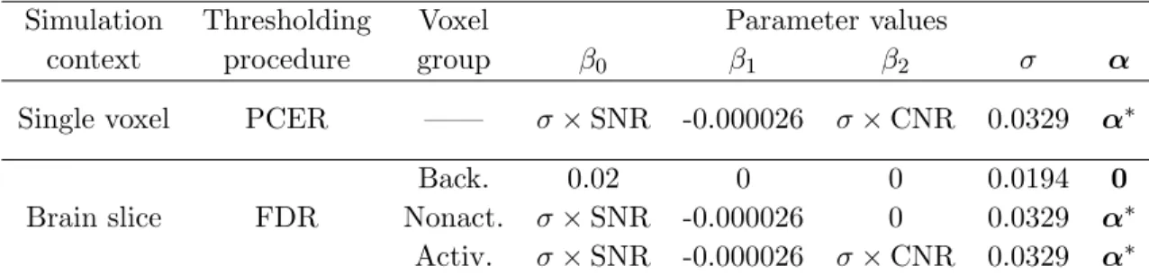
2.1 Summary of parameters used in the two contexts of simulation
experi-ments. In the above,α∗ = (0.17,0.45,−0.11,−0.23) and the voxel group abbreviations “Back.”, “Nonact.”, and “Activ.” represent background,
non-activated, and activated voxel groups, respectively. . . 17
2.2 The proportions of simulated voxel time series detecting each AR order
ˆ
punder the complex-valued and magnitude-only model order detection
procedures introduced in Section 2.3.3. The true order of 4 is shown
in bold. Results are reported under both PCER and FDR thresholding
and the PACF and LRT order detection test statistics. . . 20
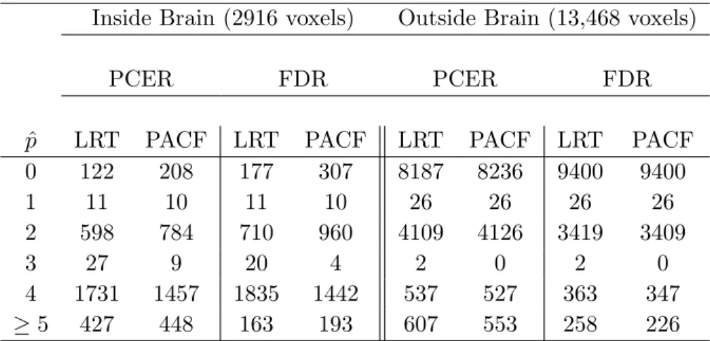
3.1 The number of voxels detecting each AR order ˆp for the finger-tapping
dataset inside and outside the brain, using PACF/LR test statistics and
PCER/FDR thresholding. . . 30
3.2 Proportion of simulated AR(0) and AR(1) complex-valued time series
detecting orders ˆp = 0,1, and greater than 1 for different values of
α1 under the LRT/PACF order detection procedures with PCER level
δ= 0.05. . . 33
4.1 Summary of the models and LRT statistics presented in Section4.2.1. 42
4.2 Computation times (in seconds) for 10,000 LRT statistics under each
model. . . 47
4.3 True detection rates of the different LRT statistics, according to an
4.4 Comparisons of ˆτG, the AUCs of ΛG, to those of the other LRT statistics,
as measured by thez-statistics described in Section4.2.2. The notation
follows that of Table4.1–e.g. zRrefers to thez-statistic calculated from
comparing the AUCs of ΛGand ΛR. Bold statistics represent significant
differences at the α= 0.05 level, after a Bonferroni adjustment. . . 51
5.1 Standard error estimates of the AR(1) Ricean estimates(a) βˆ1 and (b)
ˆ
α1 calculated from magnitude time series generated withβ1 = 0.0,α1= 0.0, and various values ofβ0. The standard errorSEbootis the standard deviation of the MLEs obtained from simulation (a bootstrap estimate), and SEemp,0.10 and SEemp,0.90 refer to the 10th and 90th percentiles of
LIST OF FIGURES
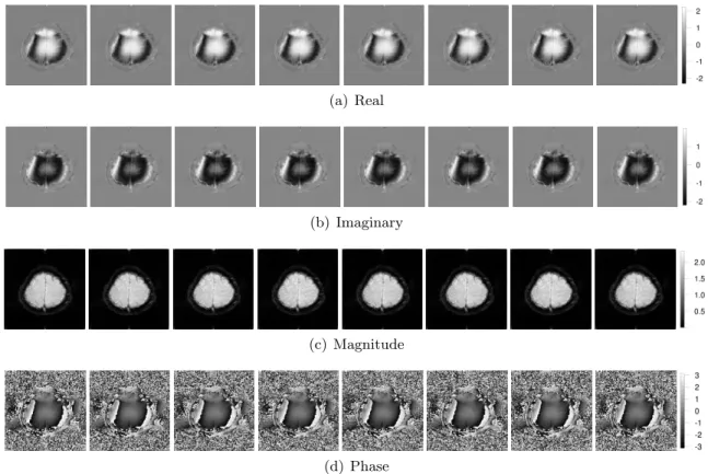
2.1 Images of the (a) real, (b) imaginary, (c) magnitude, and (d) phase
data for time points 5, 9, 13, 17, 21, 25, 29, and 33 (moving left to right), which represent the first complete 32-s cycle of the finger-tapping
experiment, containing 16-s periods of tapping and rest. . . 9
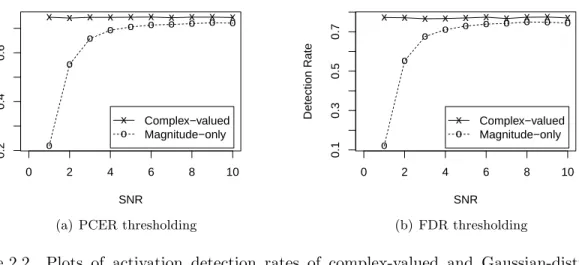
2.2 Plots of activation detection rates of complex-valued and
Gaussian-distributed magnitude model LRT statistics against SNR for (a) the
single voxel simulation context, using aδ= 0.0005 PCER level, and(b)
the brain slice context using an FDR levelq∗= 0.05. The CNR is 0.35. 18
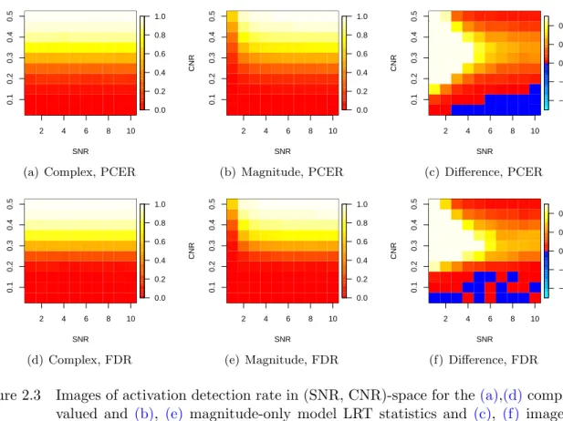
2.3 Images of activation detection rate in (SNR, CNR)-space for the(a),(d)
complex-valued and (b), (e) magnitude-only model LRT statistics and
(c),(f) images of the difference (“complex minus magnitude”) of these
rates. Simulations are performed in(a)-(c)the single voxel context with δ= 0.0005 and(d)-(f) the brain slice context with q∗= 0.05. . . 19
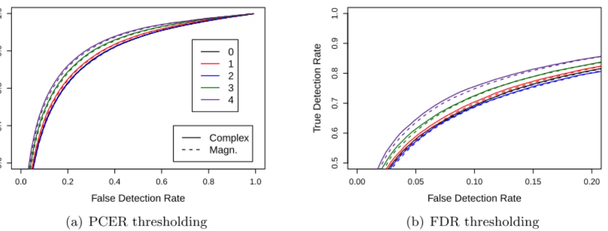
2.4 ROC curves for LRT activation statistics based on assigned orders ˆp=
0,1,2,3,4 and complex-valued and magnitude-only models under (a)
PCER and(b)FDR thresholding. . . 21
2.5 ROC curves for complex-valued- and magnitude-only-model LRT
acti-vation statistics based on detected AR orders under (a)PCER and(b)
FDR thresholding. . . 21
2.6 Plots of bias in (a) PCER (or Type I error rate) and (b) FDR versus
nominal values for prewhitening and likelihood-based, magnitude-only
2.7 Images of the detected AR orders under (a) complex-valued and (b) magnitude-only data approaches for the finger-tapping dataset, using
the LRT statistic with FDR thresholding at aq∗ = 0.05 level. . . 23
2.8 (a)Anatomical image of the subject’s brain displaying the central sulci
(in green), which contain the sensori-motor finger area cortices.
Acti-vation maps of the (b) complex-valued and (c) magnitude-only model
LRT statistics (overlayed on top of the same anatomical image), thresh-olded at the 5% false discovery rate. (Note that activation maps are drawn after masking out voxels outside the brain, as determined by the
anatomical image.) . . . 24
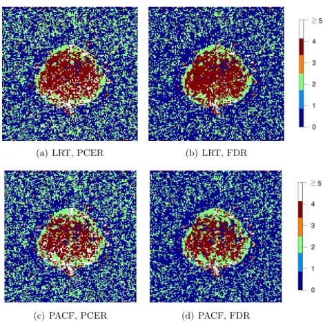
3.1 Images of the detected AR orders ˆp for the dataset, using the
complex-valued model order detection methodology described in Section 2.3.3,
under PACF/LR test statistics and PCER/FDR thresholding. . . 31
3.2 Images of complex-valued AR(4) model MLEs for the finger-tapping
data set. . . 32
3.3 Images of the PACFs computed from the real and imaginary residuals
of the finger-tapping dataset for lags 1 to 20. . . 34
3.4 Quantile-quantile plot of Box-PierceQ20-statistics for independent- and
AR(4)-model-fit residuals of the simulated and finger-tapping data
(“em-pirical”) versus a random sample from the null distribution ofQ20under
an AR(4) model,χ2
16. . . 35
4.1 Integrals of Taylor, Gaussian, Ricean, and truncated normal PDFs over
positive support for different signal parametersµ and noise parameter
σ2= 1.0. . . 42
4.2 (a)-(c)Biases,(d)-(f)standard errors (SE), and(g)-(i)root mean squared
errors (RMSE) of the unrestricted MLEs under each model plotted
4.3 False detection rates of the different LRT statistics, according to an
α= 0.05 significance level, are plotted against SNR. The legend follows
Table4.1. . . 48
4.4 The (theoretical) variance of the Rice(µ,1.0) distribution plotted against
µ(or alternatively, SNR), with estimates of the middle 95% of the
dis-tributions of ˆσ2G (obtained from simulation) at µ= 0.0,0.5, . . . ,6.0. A horizontal line atσ2G∗=σR2 = 1.0 is given for comparison. . . 49
5.1 Biases of the AR(1) Ricean- and Gaussian-model parameter estimates
are plotted againstβ0 (or alternatively, SNR) for different values of α1. 62
5.2 False detection rates at a 0.05 significance level for the (a) activation
and (b)order detection statistics are plotted againstβ0. . . 64
5.3 Areas under the ROC curve (AUCs) for the(a)activation and(b)order
detection statistics are plotted againstβ0, where “∗” denotes a statisti-cally significant difference at the 0.05 significance level after a Bonferroni adjustment. . . 64
5.4 Images of the magnitude data for time points 5, 9, 13, 17, 21, 25, 29, and
33 (moving left to right), which represent the first complete 32-s cycle of the finger-tapping experiment, containing 16-s periods of tapping and rest. . . 65
5.5 Images of the detected AR orders under (a) Ricean and (b) Gaussian
models overlayed on a contour plot of brain anatomy. . . 66
5.6 Images of theq-values associated with the voxelwise activation statistics
under(a) Ricean and (b)Gaussian models overlayed on a contour plot
ABSTRACT
Although it is well-known that data from functional magnetic resonance imaging (fMRI) experiments are complex-valued as a result of Fourier reconstruction, the vast majority of statistical analyses focus only on the magnitudes of these complex-valued measurements and discard the phase information. Moreover, most “magnitude-only” analyses rely on a Gaussian-approximation to the Ricean-distributed magnitudes, which is not (even approximately) valid
at low signal-to-noise ratios (SNRs). As a result, we advocate use of the entire
complex-valued data in statistical modeling and extend the complex-complex-valued-data model in Rowe and
Logan (2004) by applying AR(p) dependence to the real and imaginary errors. Based on
this complex-valued model, we develop a likelihood-ratio test (LRT) for detecting activated brain voxels (or volume elements) which outperforms an LRT based on a Gaussian-assumed
AR(p) magnitude-only model for simulated and experimental data. For existing fMRI datasets
with unrecoverable phase information, we advocate Ricean modeling of the magnitude data; to this end, we compare the performance of activation tests based on Ricean and Gaussian
magnitude-only models. In addition, we develop tests based on an “AR(p) Ricean” model that
augments the observed magnitude data with missing phase data in an EM algorithm framework. Somewhat surprisingly, the Ricean-based activation tests perform similarly to their Gaussian-based counterparts, even at low SNRs, which further supports the use of complex-valued data.
CHAPTER 1. INTRODUCTION
This dissertation contributes to the study of statistical modeling of functional magnetic resonance imaging (fMRI) data. Functional MRI is commonly used to study brain function because it is noninvasive, requires no exposure to radiation, and is widely available. The primary goal of statistical analysis of fMRI data is detecting the brain region(s) activated by a given stimulus or task. This is commonly done in two steps: first, the time series of measurements at each voxel (or volume element) is reduced to a test statistic which summarizes the association between each voxel time course and the expected response to the stimulus. Second, the resulting map of statistics is thresholded to identify voxels that are significantly activated. We focus on the first of these steps, developing activation statistics based complex-valued and Ricean modeling of fMRI voxel time series.
The vast majority of statistical analyses study the magnitude data computed from the complex-valued measurements resulting from Fourier reconstruction. This practice, which has carried over from structural MRI, discards the phase information. However, noting that both
components of the data are acquired, Nan and Nowak (1999) and Rowe and Logan (2004)
encourage use of both the magnitude and the phase (i.e., complex-valued) data in the analysis
and demonstrate that such analyses have greater activation detection power than
“magnitude-only” analyses at low signal-to-noise ratios (SNRs). In a paper in progress (Chapter 2), we
extend the complex-valued data model in Rowe and Logan (2004) by applying AR(p)
depen-dence to the real and imaginary error vectors, and we apply this model to fMRI data from a
finger-tapping experiment. Chapter 3is a supplement to this paper.
While we hope this will help spur the adoption of complex-valued methodology, we note that since the practice to date has been to rely on magnitude-only fMRI datasets, there are a large number of available datasets for which the phase information has been discarded. As a result,
we also consider magnitude time series, which are commonly assumed to follow a Gaussian general linear model. However, because the real and imaginary measurements are well-modeled as two independent Gaussian random variables with the same variance, the magnitude data follow the Rice distribution, which is well-approximated by the Gaussian distribution at high SNRs, but not so when the SNR is low. Consequently, Rice-distributed magnitude-only models (den Dekker and Sijbers, 2005; Rowe, 2005b; Zhu et al., 2009) have shown improved power
of detection over Gaussian models at low SNR. In Chapter 4, we expand upon these previous
studies of Ricean and Gaussian models for low-SNR fMRI magnitude time series.
In Chapter 5, we delve deeper into Ricean models by incorporating temporal dependence.
Previously, such efforts have been complicated by the fact that time series modeling is largely based upon the Gaussian distribution, a “mismatch” under Ricean models. However, we bridge
this gap by applying AR(p) errors to the Gaussian-distributed real and imaginary components
– similar to the model of Chapter 2, except that the complex-valued data are unobserved in
this magnitude-only context. This “AR(p) Ricean” model depends on augmenting the observed
magnitude data by missing phase data in an EM algorithm framework. We use the EM al-gorithm for parameter estimation and extend it to compute approximate standard errors and test statistics for activation and AR order detection. We compare the performance of this new
CHAPTER 2. IMPROVED ACTIVATION DETECTION VIA COMPLEX-VALUED AUTOREGRESSIVE MODELLING OF FMRI
VOXEL TIME SERIES
A paper in preparation
Daniel W. Adrian, Ranjan Maitra, and Daniel B. Rowe
Abstract
A complex-valued model with AR(p) errors is proposed as an alternative to the more
common Gaussian-assumed magnitude-only AR(p) model for fMRI time series.
Likelihood-ratio-test-based activation statistics are derived for both models and are compared in terms of activation detection and false discovery rates for simulated and experimental data. For
simu-lated data, the complex-valued AR(p) model likelihood-ratio activation statistic shows superior
power of activation detection at low signal-to-noise ratios and lower false discovery rates. Also, when applied to an experimental data set, the activation map produced by the complex-valued
AR(p) model more clearly identifies the primary activation regions. Our results advocate the
use of the complex-valued data and the Gaussian AR(p) model as a more efficient and reliable
tool in fMRI experiments over the current practice of using only the magnitude dataset.
2.1 Introduction
Functional magnetic resonance imaging (fMRI) is a popular method for studying brain function because it is noninvasive, requires no exposure to radiation, and is widely available. The imaging modality is built on the fact that when neurons fire in response to a stimulus or a task, the blood oxygen levels in neighboring vessels changes, effecting the magnetic resonance
(MR) signal on the order of 2-3% (Lazar,2008), due to the differing magnetic susceptibilities of oxygenated and deoxygenated hemoglobin. This difference is behind the so-called Blood
Oxygen Level Dependent (BOLD) contrast (Ogawa et al.,1990;Belliveau et al.,1991;Kwong
et al., 1992; Bandettini et al., 1993) which is used as a surrogate for neural activity and is used to acquire time-course sequences of images, with the time-course in accordance with the stimulus and resting periods.
Each MR image is obtained in a series of steps from the so-calledk-space data which encodes
different frequency contributions to each voxel. The different frequencies result from magnetic
field gradients (Jezzard and Clare,2001) and need to be inverted to localize measurements at
each voxel. This is achieved by applying the inverse Fourier transform (Jain, 1989) on the
k-space data, which results in a complex-valued observation at each voxel and each time-point.
Thus, acquired fMRI (and MR) data at each voxel and time-point can, in reality, be written in terms of its real and imaginary (alternately, magnitude and phase) components. The real and imaginary components of the acquired voxel-wise MR signal are well-modeled as two
inde-pendent normal random variables with the same variance (Wang and Lei,1994). This implies
that the magnitude measurements follow the Rice distribution (Rice,1944;Gudbjartsson and
Patz,1995), which is well-approximated by the normal distribution at high signal-to-noise ratio
(SNR), but not so when the SNR is low.
Acquired MR datasets have typically used the magnitude measurements at each voxel for display and analysis. This practice of using only the magnitude data while discarding the phase at each voxel has carried over to fMRI practice so much so that the vast majority of statistical analyses of such data completely ignore the phase data and base their inferences on
only the magnitude time series at each voxel (Rowe and Logan,2004,2005). Thus, even though
additional (phase) information is available, analysis in fMRI has almost exclusively focused on the time series of the magnitude MR data at each voxel. Indeed, as we discuss in our review of current fMRI practice, many of the methods used in such analyses assume that the magnitude time series are normally distributed, even though such observations may not all be obtained at high SNR.
— commonly a general linear model (Friston et al., 1995) – to the time series observations against a transformation of the input stimulus: this transformation is the expected BOLD response and is effectively modeled in terms of a convolution of the stimulus time course with the hemodynamic response function (HRF), which measures the delay and dispersion of the
BOLD response to an instantaneous neuronal activation (Friston et al., 1994; Glover, 1999).
This provides the setting for the application of the Statistical Parametric Mapping (SPM)
technique ofFriston et al.(1990) which was originally developed to analyze Positron Emission
Tomography (PET) time course data, but which has since been extended to become one of the most popular approaches to analyzing fMRI data. The time series at each voxel is thus reduced to a test statistic at each voxel, which summarizes the association between each voxel
time course and the expected BOLD response (Bandettini et al., 1993). The resulting map
is then thresholded to identify voxels that are significantly activated (Worsley et al., 1996;
Genovese et al.,2002;Logan and Rowe,2004).
In its simplest form, the above analysis assumes no autocorrelation within the time series: however it is widely realized that this assumption is not supported in reality. There are many reasons for this: one is that the hemodynamic response disperses (or “smears”, in fMRI jargon) neural activation. The hemodynamic (or BOLD) response to a single neural activation takes
15 to 20 seconds (Lazar,2008), which is much longer than the sampling intervals of many fMRI
techniques – 100 ms-5 s for echo-planar imaging (EPI) techniques (Friston et al.,1994). Further,
the neuronal response, which can be modeled as a point response or a delta function (Friston
et al.,1994), is itself very fast when compared to the BOLD response. Since fMRI experiments measure the BOLD response over time, the above discussion means that the observed time series
within each voxel are correlated. Friston et al. (1994) also contend that the neuronal process
is composed of “intrinsic” neuronal activities in addition to the stimulus-related response. Consequently, the authors say, autocorrelations in the observed time series arise from two neural components, both measured through the hemodynamic response: one that is experimentally induced owing to the stimulus and another that is due to intrinsic neuronal activity. The first component is modeled by the convolution of the stimulus time course with the HRF, as discussed previously, while the second is present even in the absence of stimuli. Note also
that some additional sources of autocorrelation are also provided by the subject’s cardiac and respiratory cycles (Friston et al.,2000).
Precise modeling of this temporal correlation is essential to maintaining assumed
signifi-cance levels in tests for activation (Purdon and Weisskoff, 1998). Many analyses extend the
linear model by introducing autocorrelated errors (Lazar,2008). Prewhitening these errors is
a common procedure, based on estimated autoregressive (AR) (Bullmore et al.,1996;Marchini
and Ripley, 2000) or autoregressive moving average (ARMA) (Locascio et al., 1997) models, and leading to the most efficient estimators. However, this approach can bias significance levels (Friston et al.,2000;Woolrich et al.,2001), so temporal (Worsley and Friston,1995) and spatial (Worsley et al., 2002) smoothing have been recommended for more robustness. Likelihood-based activation statistics, Likelihood-based on incorporating an AR temporal correlation structure into the likelihood function, have also been proposed as a less-biased alternative to prewhitening approaches (den Dekker et al.,2009).
The above approaches all make Gaussian distributional assumptions for the observed mag-nitude time series, which as discussed before, is not appropriate, even approximately, at low
SNR. This has led to the development of Rice-distributed magnitude-only models (den Dekker
and Sijbers,2005;Rowe,2005b;Zhu et al.,2009) which have, understandably, shown improved power of detection over their Gaussian counterparts at low SNR. Incorporating autocorrelation directly in the Rice-based models is however complicated, and the prewhitening approaches discussed above do not apply since they are based on Gaussian-distribution-based extensions of the linear model.
A different approach, advocated by Nan and Nowak (1999) and Rowe and Logan (2004),
encourages use of both the magnitude and the phase (i.e., complex-valued) data in the analysis.
Noting that both components of the data are all acquired, just not used, these authors have also demonstrated that complex-valued statistical analyses of voxel time series show a greater power of activation detection than Gaussian-distribution-assumed magnitude-only (henceforth referred to as magnitude-only in this paper, unless otherwise specified) analyses at low SNRs. In simulation studies that assume independent errors, complex-valued models have shown in-creased detection power over magnitude-only models at low SNR (of less than 5, and sometimes
even as high as 7.5), and the two have shown comparable detection power at high SNR (Rowe and Logan,2004). In addition, magnitude-only models yield biased parameter estimates at low SNR: even for large SNR, the variance of the residual variance estimates is twice that obtained
with the complex-valued model (Rowe, 2005b). These results are due to two shortcomings of
magnitude-only data analysis; first, half the data is discarded, which causes the larger variance of residual variance estimates under the magnitude-only model. Secondly, as mentioned ear-lier, the approximate Gaussian distributional assumption for Rice-distributed magnitude data is poor at low SNR. This factor is increasingly important because the SNR is proportional to
voxel volume (Lazar,2008). Thus an increase in the fMRI spatial resolution will correspond to
a lowering of the SNR, making the Gaussian distributional approximation for the magnitude data even less tenable.
Using the phase data in addition to the magnitude data in fMRI studies has proved valu-able in other ways. For one, prewhitening can occur without distributional approximation for
complex-valued data models (Rowe and Logan,2004). Time course data on the phase have also
proved useful in identifying voxels that show unwanted BOLD response due to the presence of
large draining veins (Hoogenrad et al.,1998;Menon,2002). These voxels show a task-related
phase change, while voxels with a more random orientation of blood vessels do not (Rowe,
2005a). Using a complex-valued model with constant phase assumption (Rowe and Logan,
2004) has proved successful in biasing against such voxels with large draining veins (Nencka
and Rowe,2007). In addition, the complex-valued data can permit the analysis of the original, k-space data (Rowe et al.,2009), before preprocessing induces spatial and temporal correlation
artifacts (Nencka et al., 2009), which may cloud conclusions in functional connectivity and
fMRI studies.
In this paper, we further develop the complex-valued time series analysis of fMRI data. Our
showcase application is a dataset from a finger-tapping experiment introduced in Section2.2.
We use this application as the context within which we introduce methodology that applies
an AR(p) dependence structure to the real and imaginary error vectors of the model inRowe
and Logan (2004). We derive likelihood-based activation statistics based on this model in
2.5, respectively. We also compute similar activation statistics under a Gaussian-distributed
magnitude-only model with AR(p) errors. After applying thresholding procedures, we compare
the performance of the two statistics in terms of detection probability and control of false
positive and false discovery rates. We discuss these results in Section 2.6. This paper also
has an online supplement providing further details on methodology, experimental illustrations, performance evaluations and data analysis, which serves as Chapter 3 of this document.
2.2 Detecting Activation in a Finger-Tapping Experiment
Our showcase application for this paper comes from a commonly-performed bilateral
se-quential finger-tapping experiment, as studied in Rowe and Logan (2004). In this case, the
MR images were acquired while the (normal healthy male) volunteer subject was instructed to either lie at rest or to rapidly tap fingers of both hands (hence bilateral) at the same time. The fingers were tapped sequentially in the order of index, middle, ring and little fingers. The experiment consisted of a block design with 16 s of rest followed by eight “epochs” of 16 s tapping alternating with 16 s of rest. MR scans were acquired once every second, resulting in 272 images. For this dataset, the complex and imaginary components of the time series images were not discarded, but stored along with the magnitude image commonly used in
tra-ditional fMR analysis. Figure2.1shows images of the real, imaginary, magnitude and phase
data at time pointst = 5,9, . . . ,33, which constitute the first 32-s cycle containing 16-second time periods of tapping and rest on a single axial slice through the motor cortex consisting
of 128×128 voxels. (Note that traditionally, only the magnitude images are used in fMRI
analysis, while the phase images are discarded.) For simplicity, we restrict attention in this paper to this two-dimensional slice of the dataset. These images appear not to change much in
time because, as explained in Section2.1, the BOLD stimulus response is very small compared
to the overall MR signal in all fMRI experiments. A dataset on a well-studied paradigm such as this provides us with as close to a “known” detected activation area as is possible in fMRI: numerous studies have confirmed activation in the sensori-motor finger area cortex in the cen-tral sulcus. Thus, this dataset provides us with an ideal case study for both developing and evaluating new methodology.
(a) Real
(b) Imaginary
(c) Magnitude
(d) Phase
Figure 2.1 Images of the(a) real,(b) imaginary,(c) magnitude, and(d) phase data for time
points 5, 9, 13, 17, 21, 25, 29, and 33 (moving left to right), which represent the first complete 32-s cycle of the finger-tapping experiment, containing 16-s periods of tapping and rest.
2.3 Methodological Development
We focus on the complex-valued time series at a voxel, which comprises of real and imag-inary time series observations, respectively denoted in this paper as yR = (yR1, . . . , yRn)0 and yI = (yI1, . . . , yIn)0, with n being the number of scans. For notational simplicity here, we suppress voxel-related subscripts, and denote the voxel-wise magnitude time series data as
r = (r1, . . . , rn)0, where rt =
q
yRt2 +yIt2, t= 1, . . . , n. We first briefly discuss the magnitude-only model. In doing so, we also introduce broadly the setup of our experiment.
As discussed in Section 2.1, magnitude-only fMRI time series observations at a voxel are
often analyzed by extending the linear modelr=Xβ+whereis assumed to be multivariate
normally distributed with an AR(p) dependence structure (Marchini and Ripley,2000;Bullmore
representing the baseline signal, signal drift, and the expected BOLD response. The AR(p) distribution ofis parameterized by AR coefficientsα= (α1, . . . , αp) and white noise variance σ2. Under this setting, the log-likelihood function is given by logL(α,β, σ2|r) = −n
2logσ
2−
1
2log|Rn|−
1
2σ2(r−Xβ)0R−n1(r−Xβ),whereRnis then×nmatrix such thatσ2Rn= Cov().
Unrestricted maximum likelihood estimates (MLEs) of the parametersβandσ2are then given
by ˆβ = (X0Rˆ−n1X)−1X0Rˆ−n1r and ˆσ2 = (r−Xβˆ)0Rˆ−n1(r−Xβˆ)/n, respectively, with ˆR−n1
given as a function of ˆα, i.e. as the MLE of α (Pourahmadi,2001). We obtain ˆα by solving
the system of equations: Pp
j=1( ˆdjk +jγˆj−k) ˆαj = ˆd0k, for k = 1, . . . , p, as in Miller (1995), where ˆdij =Pn−i−j
t=1 ˆt+iˆt+j, for 0 ≤ i, j ≤p, and ˆγk = ˆd0k/n, k = 0, . . . , p−1, is the lag k sample autocovariance. In the preceding discussion, ˆt=rt−xt0βˆ, where x0t is the tth row of X, t= 1, . . . , n. The estimation procedure, due to Cochrane and Orcutt (1949), begins with
ˆ
Rn=In, the identity matrix of ordern×n, and then iteratively updates ˆβ, ˆα, and ˆR
−1
n until
convergence.
A general hypothesis test for activation can be framed as H0 :Cβ =0 vs. Ha :Cβ 6=0.
(Note that this formulation of the alternative allows for “negative activation” in response to the fMRI stimulus/task at the voxel.) The likelihood ratio test (LRT) statistic is given by
−2 logλM =nlog ˜ σ2 ˆ σ2 −log ˜ R−p1 / ˆ R−p1 , (2.1)
where ˜σ2 and ˜α are restricted MLEs under H0 (see the derivations in Section 3.1.1) and ˆR
−1
p and ˜R−p1are functions of ˆαand ˜α, respectively, as inPourahmadi(2001). The null distribution of the LRT statistic (2.1) is asymptotically χ2m with m= rank(C).
2.3.1 Autoregressive modeling for complex-valued fMRI time series data
FollowingRowe and Logan (2004), our model for complex-valued fMRI voxel time series is
yR yI = X 0 0 X βcosθ βsinθ + ηR ηI . (2.2)
This formulation means that the real and imaginary time series have phase-coupled means
according to a central phase θ, fixed in the time series but allowed to vary between voxels.
and expected BOLD response. The real and imaginary error vectors, ηR and ηI, are assumed
to be independent and Gaussian-distributed with Cov(ηR) = Cov(ηI) =Σ. Rowe and Logan
(2004) specify thatΣ=σ2In, assuming that existing correlations in the time series have been
removed by the prewhitening procedure outlined in their paper. However, we assign an AR(p)
process to the real and imaginary errors, with AR coefficients α and white noise variance σ2.
Define Rn such that σ2Rn = Cov(ηR) = Cov(ηI). Under this framework, the log-likelihood
function is given by logL(α,β, θ, σ2|yR,yI) =−nlogσ2−log|Rn| −h/2σ2,where
h= yR−Xβcosθ yI−Xβsinθ 0 R−n1 0 0 R−n1 yR−Xβcosθ yI−Xβsinθ . (2.3)
Similar to the derivations in Rowe and Logan (2004), the unrestricted MLE for β is ˆβ =
ˆ
βRcos ˆθ+ ˆβIsin ˆθ, where ˆβR = (X0Rˆ
−1 n X)−1X 0ˆ R−n1yR and ˆβI = (X0Rˆ −1 n X)−1X 0ˆ R−n1yI, and ˆR−n1 is again a function of ˆα as inPourahmadi (2001). The MLE forθ is given by
ˆ θ= 1 2arctan " 2 ˆβ0RX0Rˆ−n1XβˆI ˆ βR0 X0Rˆ−n1XβˆR−βˆ0IX0Rˆ−n1XβˆI # , (2.4)
while that forσ2 is ˆσ2 = ˆh/2n, where ˆhreplaces parameters by their MLEs in (2.3). We obtain ˆ
α by solving the system of equations:
ˆ d0k= p X j=1 ( ˆdjk+ 2jˆγj−k) ˆαj, (2.5)
for k = 1, . . . , p, which is a slight modification of the system obtained in the Gaussian-assumed magnitude-only time series observations earlier. Further, ˆdij =Ptn=1−i−jηˆR,t+iηˆR,t+j+ ˆ
ηI,t+iηˆI,t+j, 0 ≤ i, j ≤ p in (2.5), and ˆγk = ˆd0k/2n is the lag-k sample autocovariance, k = 0, . . . , p−1. Also, ˆηRt = yRt−x0tβˆcos ˆθ and ˆηIt = yIt −x0tβˆsin ˆθ, t = 1, . . . , n. The ML estimation procedure thus consists of iteratively updating (ˆθ,βˆ), ˆα, and ˆR−n1 successively, proceeding until convergence.
Activation tests can be framed in the same way as before, i.e. by positing H0 : Cβ =0
againstHa:Cβ 6=0. The LRT statistic for the complex-valued AR(p) model is given by
−2 logλC = 2nlog ˜ σ2 ˆ σ2 −2 log ˆ R−p1 / ˜ R−p1 , (2.6)
where ˜α and ˜σ2 are restricted MLEs obtained under H0 and derived in Section3.1.2. Under H0, the LRT statistic is again asymptotically χ2m. Note also that the matrices ˆR
−1
p and ˜R
−1
p are functions of ˆαand ˜α, respectively, as in Pourahmadi(2001). Further, both (2.1) and (2.6)
are modifications of the LRT statistics given inRowe and Logan(2004) for AR(p) rather than
independent errors.
2.3.2 Prewhitening-based approaches to calculating activation statistics
A simpler alternative to the previous likelihood-based approaches for calculating LRT acti-vation statistics under assumptions of known covariance matrices (for both magnitude-only and complex modeled cases) is prewhitening, but because of the restrictive assumptions, resulting inferences are at best “only approximately valid” (seeden Dekker et al.,2009, who, as an alter-native, proposed LRT-based activation statistics assuming magnitude-only data and Gaussian
model.) Rowe and Logan (2004) outlined a prewhitening approach for complex-valued AR(1)
datasets. Here, we formalize and extend the above to the case where the estimated
covari-ance matrix is computed by fitting an AR(p) model to the residuals. These estimates are
used to “whiten” the data following which the MLEs and LRT-based activation statistics are
calculated. The latter is illustrated in Rowe and Logan (2004), which assumes temporal
in-dependence within the time series at a voxel; thus, here we describe only how to obtain the
“whitened” data. First, the AR order p is estimated using methodology described in Section
2.3.3. Estimates of AR coefficients can then be obtained from (2.5), following which R−n1 can
be estimated using R∗−n1 as in Section 2.3.1. Write R∗−n1 = QQ0 in terms of its Cholesky
factorization. Then (y∗R,y∗I)0 =I2⊗Q(y0R,y0I)0, with⊗representing the Kronecker product, is
assumed to be multivariate normally distributed with mean vector (cosθ,sinθ)0⊗(QXβ) and
covariance matrix σ2I2n, and forms the “whitened” data. In comparison with the
likelihood-based procedure, which iteratively updates (ˆθ,βˆ), ˆα, and ˆR−n1 until convergence of the ML estimates, prewhitening essentially “stops” after the first iteration. As a result, prewhitening requires less computation than the likelihood-based procedure, but, as mentioned above, makes “only approximately valid” inferences.
2.3.3 Choosing the order of the autoregressive model
The order of the AR(p) models, whether for the magnitude-only or the complex-valued
case, is not a priori known and needs to be determined. We propose sequentially testing
H0 : αk = 0 vs. Ha : αk 6= 0, starting with k = 1, for increasing k. Let k0 be the first k in the sequence of tests for which the null hypothesis can not be rejected. Then the estimated AR(p) order is given by ˆp=k0−1. We propose two alternative test statistics for carrying out each test: the (sample) partial autocorrelation function (PACF) and, separately, another LRT statistic for order detection. Both of our test statistics are extensions to the complex-model case of the usual magnitude-only version. In the latter case, the PACF is calculated from the
magnitude-only residualsˆassuming independence. Shumway and Stoffer (2006) show that for
an AR(p) process of n observations, the lag-ksample PACF ˆakk has an asymptotic N(0,1/n)
distribution, fork > p. The null distribution of the magnitude-only PACF statistic ˆa(kkM)is then
approximately N(0,1/n). Extension to the complex-valued fMRI time series case essentially
involves combining the contributions from the real and imaginary residuals, resulting in our proposed PACF test statistic ˆa(kkC)= ˆakk(R)+ ˆa(kkI), the sum of the lag-kPACFs computed from the real and imaginary parts of the residuals. These residuals are computed as ˆηR=yR−Xβˆcos ˆθ and ˆηI =yI −Xβˆsin ˆθ, respectively, where ˆβ and ˆθ are as in Section 2.3.1, with ˆR−n1 =In.
Because these residuals are independent (see Section 3.2), the PACF statistic has a N(0,2/n)
distribution under H0.
The alternative LRT-based test statistic is given by the usual 2(ˆ`k −`ˆk−1) where ˆ`k is
the optimized log-likelihood for the (magnitude-only or complex-valued) AR(k) model: from
standard results, this test statistic is asymptoticallyχ21-distributed underH0.
The decision on whether to continue testing in the sequential procedure outlined above can be based on either standard per-comparison error rate (PCER) methodology or false discovery
rate (FDR) thresholding (Benjamini and Hochberg, 1995). The latter accounts for multiple
significance assessments in order detection. For PCER thresholding, we base these single-test
decisions by specifying the probability of Type I error, which is rejecting H0 : αk = 0 when
the detected order is over-specified, given that it is not underspecified. To show this, recall that the detected order ˆp=k0−1, wherek0is the firstkfor which we are unable to rejectH0 :αk= 0. Note two facts: first, rejecting H0 :αk = 0 means that k0 > k ⇒ p > kˆ −1. Second, simply
testing H0 :αk = 0 in the context of the procedure implies thatk0 ≥k⇒pˆ≥k−1. From the
definition ofδ, for k > p,δ= Pr(ˆp > k−1|pˆ≥k−1). Substitutingk=p+ 1 yields the above result.
We now describe simultaneous detection of the order in M voxel time series using FDR
thresholding. For m = 1, . . . , M, denote αmk be thekth order AR coefficient. For increasing
k, starting at k = 1, we simultaneously test H0 :αm(k)k = 0 vs. Ha :αm(k)k 6= 0, for m(k) =
1, . . . , Mk. For each of theMk voxel time series,p-values (i.e., the measure of evidence against
H0 – not AR order) are computed from one of the discussed test statistics and decisions are
based on the “Bonferroni-type” FDR controlling procedure given in Benjamini and Hochberg
(1995). For k= 1, allM voxel time series are tested; that is, M1 =M. Letk0m be the first k
for which the time series at the mth voxel fails to reject H0. Then the detected order for this
voxel time series is ˆpm=k0m−1. For increasing k, the number of tested voxel time seriesMk
decreases as voxels with k0m < k (whose AR order has already been determined) are excluded
from tests. That is, Mk+1 =Mk−Gk, where Gk is the number of voxels with “fail to reject
H0” decisions for order k. Simultaneous tests continue for increasing k until Mk = 0. The
FDR levelq∗ is the rate at which the null hypothesis is rejected in error: thus, in the context
of simultaneous order detection, it is the rate at which the order is detected in error (actually over-specified).
2.3.4 Detecting voxels significantly activated by the stimulus
Having detected the order of the fitted autoregressive models, our task now is to detect activation, which is really the primary goal of our experiment. As mentioned previously, a
general test for activation for a single voxel time series is H0 : Cβ = 0 vs. Ha : Cβ 6=
0. Each voxel is identified as activated if H0 is rejected, whether for the magnitude-only or
complex-valued AR(p) model: in either case, given the order p, the tests are asymptotically
χ2
thresholding, with the latter accounting for the multiple testing issues introduced when multiple voxels are considered.
2.4 Experimental Evaluations
We applied the methodology in Section 2.3, computing LRT activation statistics for
sim-ulated fMRI data under both magnitude-only and complex-valued models with AR(p) errors.
We simulated complex-valued voxel time series in a manner so as to mimic the experiment
of Section 2.2, obtaining magnitude time series versions of them in the same way as is done
in fMRI. Our simulation setup used the model (2.2) with our X-matrix matching that of the
experiment in Section 2.2. Specifically, our design matrix X contained q = 3 columns: the
first column denoted the intercept term, the second modeled linear drift in the signal, while
the third modeled the expected BOLD response with a ±1 square wave. (Note that
conse-quently, with β = (β0, β1, β2)0, activation tests were equivalent to testing H0 :β2 = 0 against Ha:β2 6= 0: also, the LRT activation statistics areχ21-distributed underH0.) The square wave
was lagged five time points (i.e. 5 seconds) from the stimulus time course to model the lag
induced by the BOLD response, as discussed in Section 2.1; compared with other lags, the lag
of five produced the highest activation statistics in the experimental dataset. Due to concerns about the constant phase assumption, we removed the first 12 and the last four time points,
leaving us with voxel time series of length n = 256. This X-matrix was used in simulating
datasets and evaluating the performance of our methodology in this section as well as in the analysis of our dataset in Section2.5.
We compared the performance of LRT activation statistics under magnitude-only and
complex-valued AR(p) models in terms of maximizing and minimizing true and false detection
rates, respectively. We emphasize three contexts of this comparison in Sections2.4.1-2.4.3, also expanding upon previous work in each. First, we examine the case with low SNR, building upon simulation experiments that, under the assumption of temporally independent (or prewhitened) voxel time series, have shown superior detection rate of complex-valued model activation
statis-tics over their Gaussian-distributed magnitude-only counterparts (Nan and Nowak,1999;Rowe
activation detection performance of both LRT statistics is affected by errors in order detection.
As discussed in Section2.1, the effect of modeling temporal dependence on activation detection
has a long history for magnitude-only fMRI time series (Lazar,2008) which we also examine
for complex-valued data. Last, we compare the bias in significance levels for likelihood-based and prewhitening-based activation statistics. Such bias, which has long been a criticism of prewhitening approaches to fMRI magnitude time series, is also computed for complex-valued data.
In each of the experiments described above, we simulated fMRI datasets and computed activation detection rates in two ways. First, we generated voxel time series from the same parameters repeatedly and used standard (PCER) thresholding to determine activation. We call this the “single voxel” simulation context. However, real fMRI datasets contain numerous voxel time series and activation detection must account for multiple testing. Thus, we also
gen-erated brain slices of 128×128 voxel time series and, in this “brain slice” context, used FDR
thresholding to determine activation. These simulated brain slices were designed to represent
the finger-tapping dataset of Section 2.2 and contained three groups of voxels: background
(outside the brain) and inactivated and activated brain voxels. Each slice contained 275 acti-vated voxels, a number estimated from the dataset. Further, we chose our parameter values to be the same for voxels in each group but different from those in other groups.
The parameter values used in each simulation context are given in Table 2.1, which are
obtained from their estimates in the finger-tapping dataset as described in Section3.3. In this
section, values of β0 and β2 are parameterized through the signal-to-noise ratio, SNR≡β0/σ,
and the contrast-to-noise ratio, CNR ≡ β2/σ, respectively. The SNR measures the size of
baseline, non-BOLD signal relative to the noise level, and the CNR measures the relative size
of the BOLD response. In Section 2.4.1, we simulate at SNR less than 10, but otherwise we
use SNR = 50, the approximate estimate from the dataset in Figure3.2(f). Since the low-level
finger-tapping task has a higher CNR than high-level tasks of interest, such as cognition, we
Simulation Thresholding Voxel Parameter values
context procedure group β0 β1 β2 σ α
Single voxel PCER —— σ×SNR -0.000026 σ×CNR 0.0329 α∗
Brain slice FDR
Back. 0.02 0 0 0.0194 0
Nonact. σ×SNR -0.000026 0 0.0329 α∗
Activ. σ×SNR -0.000026 σ×CNR 0.0329 α∗
Table 2.1 Summary of parameters used in the two contexts of simulation experiments. In the
above, α∗ = (0.17,0.45,−0.11,−0.23) and the voxel group abbreviations “Back.”, “Nonact.”, and “Activ.” represent background, non-activated, and activated voxel groups, respectively.
2.4.1 Complex-valued/magnitude-only activation detection at low SNR
As noted in Section 2.1, SNR is proportional to voxel volume, so fMRI studies with
in-creased spatial resolution will have lower SNR data. We simulate such fMRI datasets with SNR = 1,2, . . . ,10 and CNR = 0.05,0.10, . . . ,0.50, generating 100,000 single voxel time series and 100 brain slices at each (SNR, CNR) combination. Assuming correct order detection, LRT activation statistics are computed under complex-valued and magnitude-only models.
Activa-tion is detected at PCER and FDR thresholds of δ = 0.0005 and q∗ = 0.05, respectively, and
detection rate is computed as the proportion of the activated simulated voxel time series (i.e.
with positive CNR) detected as such. These activation detection rates are plotted against SNR
for CNR = 0.35 in Figure2.2, which shows striking similarity to those for simulated temporally
independent voxel time series (compare withRowe and Logan,2004, Figure 12). The activation
detection rate is constant in SNR for the complex-valued model LRT statistic, but decreases at
low SNR under the Gaussian-distributed magnitude-only model. As discussed in Section 2.1,
the latter is most likely owing to the poor Gaussian approximation of the Rice-distributed mag-nitude observations at low SNR. This distributional approximation appears more tenable for
SNR≥6 because the magnitude-only model detection rate is constant over this range, though
at a slightly lower level than the complex-valued model. We ascribe this slight difference to the disposal of the phase information under the magnitude-only model.
Figure 2.3summarizes the relationship between detection rate and SNR for all the CNRs
complex-x x x x x x x x x x 0 2 4 6 8 10 0.2 0.4 0.6 SNR Detection Rate o o o o o o o o o o x o Complex−valued Magnitude−only
(a) PCER thresholding
x x x x x x x x x x 0 2 4 6 8 10 0.1 0.3 0.5 0.7 SNR Detection Rate o o o o o o o o o o x o Complex−valued Magnitude−only (b) FDR thresholding
Figure 2.2 Plots of activation detection rates of complex-valued and Gaussian-distributed
magnitude model LRT statistics against SNR for (a) the single voxel simulation
context, using aδ = 0.0005 PCER level, and (b) the brain slice context using an
FDR levelq∗= 0.05. The CNR is 0.35.
valued and magnitude-only LRT statistics and for the differences in their detection rates. The features in the detection rate by SNR relationship discussed in the previous paragraph are again present, most prominently for moderate CNRs; the differences in activation detection rates again vanish for low and high CNRs, as detection rates are then close to zero and one,
respectively, regardless of model and SNR. Note that the negative differences in Figures2.3(c)
and (f) (which favor the magnitude-only model), though visually compelling, represent very
small differences: the largest is less than 0.1%.
2.4.2 AR order detection errors and their consequences on activation detection Before investigating the effects of AR order detection errors on the performance of the LRT activation statistics, we examine the rates of such errors under complex-valued and
magnitude-only models. Using the parameters in Table 2.1 and a true AR order of p = 4, we simulate
100,000 single voxel time series and 100 brain slices with zero CNR and SNR = 50. We apply
the order detection methods introduced in Section 2.3.3 (tested for other simulated datasets
in Section 3.4), using PCER and FDR levels δ = q∗ = 0.05. The proportions of voxel time
series detecting each order are shown in Table 2.2, which only includes in-brain voxels for the
simulated brain slices. Magnitude-only model order detection procedures have error rates more than double those for complex-valued model procedures. This is not surprising, considering
2 4 6 8 10 0.1 0.2 0.3 0.4 0.5 SNR CNR 0.0 0.2 0.4 0.6 0.8 1.0
(a) Complex, PCER
2 4 6 8 10 0.1 0.2 0.3 0.4 0.5 SNR CNR 0.0 0.2 0.4 0.6 0.8 1.0 (b) Magnitude, PCER 2 4 6 8 10 0.1 0.2 0.3 0.4 0.5 SNR CNR −0.04 −0.02 0.00 0.02 0.04 (c) Difference, PCER 2 4 6 8 10 0.1 0.2 0.3 0.4 0.5 SNR CNR 0.0 0.2 0.4 0.6 0.8 1.0 (d) Complex, FDR 2 4 6 8 10 0.1 0.2 0.3 0.4 0.5 SNR CNR 0.0 0.2 0.4 0.6 0.8 1.0 (e) Magnitude, FDR 2 4 6 8 10 0.1 0.2 0.3 0.4 0.5 SNR CNR −0.04 −0.02 0.00 0.02 0.04 (f) Difference, FDR
Figure 2.3 Images of activation detection rate in (SNR, CNR)-space for the(a),(d)complex–
valued and (b), (e) magnitude-only model LRT statistics and (c), (f) images of
the difference (“complex minus magnitude”) of these rates. Simulations are per-formed in (a)-(c) the single voxel context with δ = 0.0005 and (d)-(f) the brain slice context withq∗= 0.05.
that complex-valued model order detection methods use twice the amount of information than the magnitude-only model detection. (Note also that most order detection errors constitute underspecification.)
Based on assigned orders ˆp = 0,1, . . . ,8, we compute LRT activation statistics for
simu-lated AR(4) voxel time series with SNR = 50 and CNR = 0.2. These activation statistics were
thresholded at various PCER and FDR levels to obtain the receiver operating characteristic
(ROC) curves in Figure2.4, which plot true detection rate against false detection rate. In ROC
plots, better performing statistics will be closer to the top and left, indicating higher true detec-tion rates and lower false detecdetec-tion rates, respectively. Under this criterion, the complex-valued and magnitude-only model statistics based on the correct orders perform best while statistics based on under-detected orders show inferior performance, while those for over-detected or-ders are indistinguishable from the correct order curves (and therefore not shown); thus, it
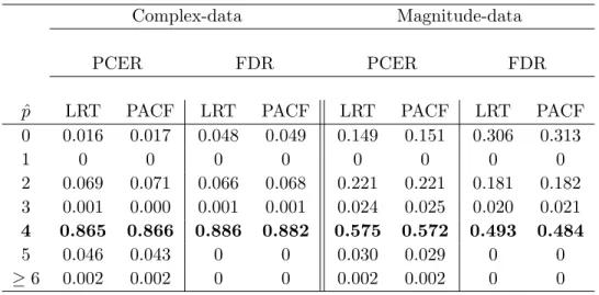
Complex-data Magnitude-data
PCER FDR PCER FDR
ˆ
p LRT PACF LRT PACF LRT PACF LRT PACF
0 0.016 0.017 0.048 0.049 0.149 0.151 0.306 0.313 1 0 0 0 0 0 0 0 0 2 0.069 0.071 0.066 0.068 0.221 0.221 0.181 0.182 3 0.001 0.000 0.001 0.001 0.024 0.025 0.020 0.021 4 0.865 0.866 0.886 0.882 0.575 0.572 0.493 0.484 5 0.046 0.043 0 0 0.030 0.029 0 0 ≥6 0.002 0.002 0 0 0.002 0.002 0 0
Table 2.2 The proportions of simulated voxel time series detecting each AR order ˆpunder the
complex-valued and magnitude-only model order detection procedures introduced
in Section 2.3.3. The true order of 4 is shown in bold. Results are reported under
both PCER and FDR thresholding and the PACF and LRT order detection test statistics.
appears that under-specifying the order has more severe consequences on activation detection
than over-specifying it. Note also that for each assigned order ˆp, the complex-valued model
activation statistic shows (slightly) higher performance than its magnitude-only counterpart. The previous results indicate that order detection errors effect the activation detection performance of the magnitude-only model more adversely than the complex-valued model. Order detection error rates were higher under the magnitude-only model and mostly consti-tuted underspecification, which was shown to cause poorer activation detection. Further, the complex-valued model LRT showed higher performance when the order was controlled. Figure
2.5, which shows ROC curves for LRT statistics based on detected orders, demonstrates the
consolidation of such effects.
2.4.3 Investigating bias in significance levels for prewhitening- and likelihood-based activation statistics
Historical concerns for prewhitening-based approaches to computing activation statistics
have centered around bias in significance levels (Friston et al., 2000), with likelihood-based
activation statistics suggested as a possible remedy (den Dekker et al.,2009). In this section, we compute both prewhitening- and likelihood-based LRT activation statistics, assuming perfect
0.0 0.2 0.4 0.6 0.8 1.0 0.6 0.7 0.8 0.9 1.0
False Detection Rate
T
rue Detection Rate
Complex Magn. 0 1 2 3 4
(a) PCER thresholding
0.00 0.05 0.10 0.15 0.20 0.5 0.6 0.7 0.8 0.9 1.0
False Detection Rate
T
rue Detection Rate
(b) FDR thresholding
Figure 2.4 ROC curves for LRT activation statistics based on assigned orders ˆp= 0,1,2,3,4
and complex-valued and magnitude-only models under (a) PCER and (b) FDR
thresholding. 0.0 0.2 0.4 0.6 0.8 1.0 0.5 0.6 0.7 0.8 0.9 1.0
False detection rate
T
rue detection r
ate
Complex−valued Magnitude−only
(a) PCER thresholding
0.0 0.2 0.4 0.6 0.8 0.0 0.2 0.4 0.6 0.8 1.0
False detection rate
T
rue detection r
ate
(b) FDR thresholding
Figure 2.5 ROC curves for complex-valued- and magnitude-only-model LRT activation
statis-tics based on detected AR orders under(a) PCER and(b)FDR thresholding.
order detection, and measure their bias in PCER and FDR levels. Our studies are over 100,000 simulated single voxel time series with zero CNR and 1000 simulated brain slices with CNR = 0.2, again at SNR = 50.
Figure 2.6 shows the significance level bias (“estimated minus nominal”) against nominal
significance level for PCER and FDR thresholding. For PCER thresholding, the estimated significance level is the Type I error rate –i.e. the proportion of non-activated voxels detected as activated. For FDR thresholding, we calculate the proportion of detected voxels (as activated) which are non-activated. To summarize, all LRT activation statistics show bias, which may be partially attributed to the asymptotic specification of their null distributions. All bias is in the
0.00 0.02 0.04 0.06 0.08 0.10 0.000 0.005 0.010 0.015 0.020
Nominal PCER level
PCER bias
Complex PW Complex Magn. PW Magn.
(a) PCER thresholding
0.02 0.04 0.06 0.08 0.10 0.01 0.03 0.05 0.07 Nominal FDR FDR bias Complex PW Complex Magn. PW Magn. (b) FDR thresholding
Figure 2.6 Plots of bias in (a) PCER (or Type I error rate) and (b) FDR versus nominal
values for prewhitening and likelihood-based, magnitude-only and complex-valued model LRT statistics.
positive direction, where more false detections occur than are nominally specified. However, the likelihood-based and complex-valued model statistics show less bias than the prewhitening-based and magnitude-only statistics, respectively. Note also that bias sizes are larger under FDR thresholding than PCER thresholding.
The results also present a third advantage of the complex-valued model LRT statistic over its magnitude-only counterpart, even when the effects of low SNR and order detection are controlled: the magnitude-only statistic has a higher false detection rate. False detection rates are also higher for prewhitening versus likelihood-based approaches, an example of the “only
approximately valid” inference based on prewhitening (den Dekker et al.,2009).
The results of all our simulation experiments demonstrate three advantages of activation detection via the complex-valued model over the Gaussian-distributed magnitude-only model: higher (true) detection rate at low SNR, smaller decrease in detection performance due to order detection errors, and smaller false detection rate. The first, which is perhaps most striking, is due to the untenable Gaussian approximation to the Rice-distributed magnitudes at SNRs below 5. The SNR for finger-tapping dataset is well above this range, so we will not see such an
effect for it, but, as mentioned in Section2.1, the SNR will decrease for datasets incorporating
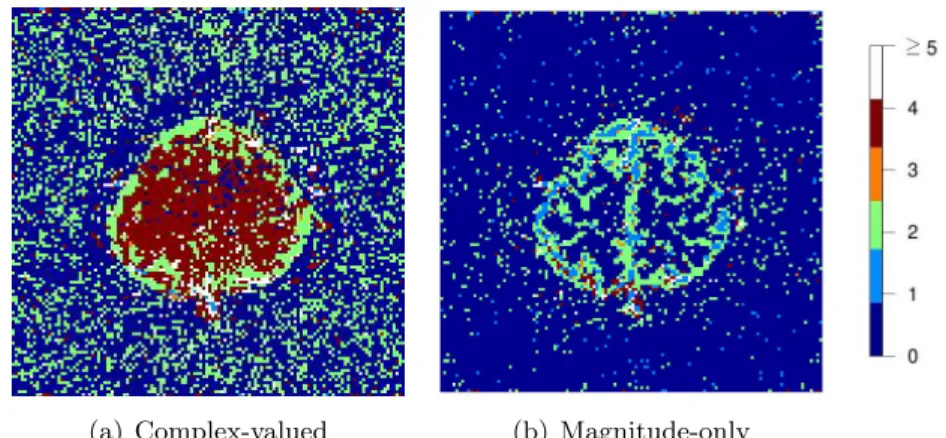
(a) Complex-valued (b) Magnitude-only
Figure 2.7 Images of the detected AR orders under (a) complex-valued and (b)
magni-tude-only data approaches for the finger-tapping dataset, using the LRT statistic with FDR thresholding at aq∗ = 0.05 level.
2.5 Application to fMRI dataset
We detected activated voxels for the finger-tapping dataset under both the complex-valued
and magnitude-only models. We used the model matrix X described in Section 2.4 in this
application. Our computation of functional activation had three steps: order detection, com-putation of LRT activation statistics, and thresholding. First, we detected the AR order for each voxel time series, applying the magnitude-only and complex-valued model procedures
pre-sented in Section 2.3.3. As shown in Figure 2.7, inside the brain, the complex-valued model
primarily detected an order of four while the magnitude-only model mostly detected zero or
two. Based on these detected orders, LRT activation statistics for the test of H0 :β2 = 0 vs.
Ha:β2 6= 0 were calculated for both models. The voxel-wisep-values, computed from the χ21
null distribution, were thresholded at a q∗ = 0.05 FDR level, determining whether each voxel
was detected. The resulting activation maps for complex-valued and magnitude-only statistics
are shown in Figures 2.8(b)and 2.8(c), respectively. On them, only detected activated voxels
are colored – with intensities according to the size of the activation statistic – and are overlayed on top of the greyscale anatomical image. Thus, our displayed activation maps display both the location of voxels detected and their “degree” of activation, where larger activation statistics demonstrate stronger activation.
(a) Anatomical Image (b) Complex-valued model (c) Magnitude-only model
Figure 2.8 (a)Anatomical image of the subject’s brain displaying the central sulci (in green),
which contain the sensori-motor finger area cortices. Activation maps of the (b)
complex-valued and(c)magnitude-only model LRT statistics (overlayed on top of
the same anatomical image), thresholded at the 5% false discovery rate. (Note that activation maps are drawn after masking out voxels outside the brain, as determined by the anatomical image.)
AR(p) model assumptions for the dataset. Since the assumptions that the real and imaginary
observations are normally distributed and uncorrelated, with the same variance have already
been established in general for MR (seee.g.Wang and Lei,1994) and specifically (see Figures
2 and 5 in Rowe and Logan, 2004) for this dataset, we focus on the assumption that the real
and imaginary errors share a common AR(p) dependence structure by noting the similarities
of the images of the voxel-wise PACFs for the real and imaginary residuals shown in Section
3.5. We also investigated, in the same section, whether an AR(p) model sufficiently removes
this temporal dependence by computing Box-Pierce statistics (Box and Pierce,1970) for
inde-pendent and AR-model-fitted residuals from the finger-tapping dataset. Results reported there show that the AR model greatly reduces the autocorrelation present, but more sophisticated time series methods may be necessary to accurately model the dependence structure in the time series.
We now discuss our findings and the relative advantages of using the complex-valued model over magnitude-only analysis. As indicated earlier, the finger-tapping task has well-established fMRI-detected activation regions in the central sulci, which are identified on the anatomical
im-age in Figure2.8(a). We argue that the complex-valued model activation map of Figure2.8(b)
both activation maps detect regions of voxels containing the central sulci, the one obtained using the complex-valued model identifies the central sulci more clearly. Also, voxels detected outside the central sulci in the complex map, better adhere to grey matter (shown lighter in
Figure 2.8(a)), which is intrinsically where neural activation takes place. Our maps may also
be compared to those in Figure 6 ofRowe and Logan(2004), which are computed (for the same
dataset) under the assumption of temporal independence. Our maps, under both complex-valued and magnitude-only models, identify the central sulci more clearly, which we attribute
to modeling the AR(p) independence. Thus, we see improved detection and localization
abil-ities in using the time series information, which is enhanced when we use the complex-valued observations over the magnitude-only datasets.
2.6 Discussion
In this paper, we have further developed the complex-valued time series analysis of fMRI data for use in fMRI data analysis. As explained here, fMRI datasets are really complex-valued when collected, but most analysis methods routinely discard the phase information, utilizing only the magnitude images in the data analysis. In doing so, current practice has been to assume a Gaussian distribution for the magnitude data, a supposition that is not even approximately correct for low SNR values. This last point is important to note because SNR (being proportional to voxel volume) decreases with increased spatial resolution. In this
paper therefore, we have proposed an AR(p) model for complvalued time series, thus
ex-tending the independent model of Rowe and Logan (2004). Under this model framework, we
derived an LRT statistic for detecting activated brain voxels. We compared its performance to a statistic similarly derived under a Gaussian-assumed magnitude-only linear model with
AR(p) errors. For low-SNR simulated data, the complex-valued statistic demonstrates notably
higher activation detection rates than the Gaussian magnitude-only statistic, due to the inaccu-racy of the normal approximation to the Rice-distributed magnitude data. This is potentially advantageous especially for the case of fMRI datasets collected at higher spatial resolutions and for datasets with higher-level cognitive tasks. In either cases, SNR and CNR values are lower and thus, there is a greater payoff for using the complex-valued approaches. Even for
high-SNR simulated data, the complex-valued approach yields lower AR order detection error rates (which negatively affect activation detection) and lower false activation detection rates, simply due to the availability of twice as many quantities in the complex-valued setting. For the finger-tapping dataset, the activation map for the complex-valued statistic more clearly identifies brain regions known to be associated with finger movement – evidence which also indicates a lower false detection rate. Aside from the major focus on complex-valued versus magnitude-only methods, we also demonstrated that prewhitening-based activation statistics produce higher false detection rates than likelihood-based statistics.
There are several aspects of our work that require further attention. For one, our AR(p)
modeling was seen to not be entirely adequate in modeling model the correlation structure with regard to the finger-tapping experimental dataset. This means that more sophisticated time series methods may be needed to completely model the temporal dependence, as revealed by the diagnostic checks. Possible extensions may be to add a moving average component to the autoregressive model and/or to introduce a seasonal component related to the periodicity in the application of the stimulus. More fundamentally, the errors may not be stationary and, if so, cannot be properly modeled using stationary methods. Secondly, we have evaluated and demonstrated performance on a dataset with high SNR in order to establish the validity of our methodology: it would be interesting to also evaluate performance on a low-SNR experimental dataset. There is some scope for optimism here, given the results of our simulation experiments and the fact that our modeling is more accurate than a Gaussian-approximated magnitude-only time series approach which is actually more suspect at lower SNR. Finally, while we hope that our methods and applications here will spur the adoption of complex-valued methodology for fMRI datasets, we note that since the practice to date has been to rely on magnitude-only fMRI datasets, there are a large number of available datasets for which the phase information has been discarded. For such datasets, temporal models that correctly model the time series in terms of the Rice distribution are needed. It is our view that complex-valued data analysis should become the norm in fMRI: however, for the these datasets, methods on Rice-distributed regression time series that accurately model the temporal correlation also need to be developed. Thus, we note that while we have presented a compelling case for incorporating complex-valued
CHAPTER 3. SUPPLEMENT TO “IMPROVED ACTIVATION DETECTION VIA COMPLEX-VALUED AUTOREGRESSIVE
MODELLING OF FMRI VOXEL TIME SERIES”
3.1 MLEs of parameters under Null Models
3.1.1 Restricted MLEs under magnitude-only autoregressive model
Under the magnitude-only AR(p) model, the restricted MLEs under H0 : Cβ =0 follow
the equations ˜ β = Ψ(X0R˜−n1X)−1X0R˜−n1r, ˜ σ2 = (r−Xβ˜)0R˜−n1(r−Xβ˜)/n, ˜ d0k = p X j=1 ( ˜djk+jγj˜−k) ˜αj, k= 1, . . . , p,
whereΨand ˜R−n1are as in Section3.1.2below. Further, ˜dij =Pnt=1−i−j˜t+i˜t+j for 0≤i, j≤p, where ˜t=rt−x0tβ˜,t= 1, . . . , n, and ˜γk= ˜d0k/n, fork= 0, . . . , p−1.
3.1.2 Restricted MLEs under complex-valued autoregressive model
Under the complex-valued AR(p) model, similar to the results inRowe and Logan (2004),
the restricted MLEs under H0 :Cβ= 0 follow the equations
˜ β = Ψ[ ˜βRcos ˜θ+ ˜βIsin ˜θ] ˜ θ = 1 2arctan " 2 ˜β0RΨ0X0R˜−n1Xβ˜I ˜ β0RΨ0X0R˜n−1Xβ˜R−β˜0IΨ0X0R˜−n1Xβ˜I # , ˜ d0k = p X j=1 ( ˜djk+ 2jγ˜j−k) ˜αj, k= 1, . . . , p,