University of Toronto
Department of Economics
November 19, 2010
By Juan Carlos Escanciano and Chuan Goh
Specification Analysis of Structural Quantile Regression
Models
Specification Analysis of Structural Quantile
Regression Models
Juan Carlos Escanciano
∗Indiana University
Chuan Goh
†University of Toronto
First draft: 14 December 2009
This version: 23 September 2010
‡∗Department of Economics, Indiana University, 105 Wylie Hall, 100 S. Woodlawn Ave., Bloomington, IN, U.S.A., 47405-7104. [email protected],http://mypage.iu. edu/˜jescanci.
†Department of Economics, University of Toronto, Max Gluskin House, 150 St. George St., Toronto, ON, Canada, M5S 3G7. [email protected], http://www. chuangoh.org.
‡This paper was initiated during Goh’s year-long visit to the Department of Economics, Indiana University. He would particularly like to acknowledge the faculty and staff of that department for their hospitality and support.
Abstract
This paper introduces a broad family of tests for the hypothesis of lin-earity in parameters of functions that are identified by conditional quan-tile restrictions involving instrumental variables. These tests are tantamount to assessments of lack of fit for quantile regression models involving en-dogenous conditioning variables, and may be applied to assess the validity of post-estimation inferences regarding the counterfactual effect of endoge-nous treatments on the distribution of outcomes. We show that the use of an orthogonal projection on the tangent space of nuisance parameters at each quantile index improves power performance and facilitates the simulation of critical values via the application of simple multiplier-type bootstrap proce-dures. Monte Carlo evidence is included, along with an application to an empirical analysis of the structure of demand for a particular subsegment of the market for anti-bacterial drugs in India.
JEL Classification: C12, C31, C52
1
Introduction
Let Y be a random variable, and let X andZ bed- and k-dimensional random vectors, respectively, wherek≥d. Consider the continuum of conditional proba-bility restrictions given by
P [Y ≤X⊤β0(α)Z
]
=α, α∈(0,1), (1) where β0(·)is measurable unknown function from [0,1] to a compact subset of Rd. As such, (1) denotes a continuum of linear-in-parameters quantile-regression
models in which the covariate vector X is possibly endogenous and Z is the corresponding vector of instruments. The identifiability of the interest parameter β0(·)in the context of (1) was shown by Chernozhukov and Hansen (2005)
un-der a conditional rank invariance condition applied to Y −X⊤β0(α) for each α ∈ (0,1).1 Estimators of β0(α) in the context of (1) have been developed
by Amemiya (1982); Powell (1983); Chen and Portnoy (1996); Honor´e and Hu (2004); Chernozhukov and Hansen (2006); Ma and Koenker (2006); Lee (2007) and Sakata (2007), amongst other authors. The “structural quantile-regression” model denoted by (1) has become increasingly popular in applied econometric analysis over the past decade. Recent applications can be found in the papers of Chernozhukov and Hansen (2004); Machado and Mata (2005); Forbes (2008) and Chernozhukov et al. (2009).
This paper develops tests for the linearity in parameters of the structural quan-tile function X⊤β0(·)in (1) over(0,1).2 As such, the hypothesis is that the
con-tinuum of conditional moment restrictions implied by (1) holds with probability one for some β0(·) in the corresponding parameter space, while the alternative
is that there is at least one quantile α′ ∈ (0,1) such that for almost every z in the support of Z, the relation given above in (1) does not hold for any vector β0(α′) ∈ Rd. Such tests are important in applications because the conclusions
of any post-estimation inferences based on estimates of β0(·) will be sensitive
to the implicit assumption that the structural quantile function in (1) is linear in parameters for all quantilesα ∈(0,1).3
1In particular, for each quantile indexα∈(0,1),Y −X⊤β
0(α)needs to be at least
distribu-tionally invariant across different realizations ofZ.
2Although the analysis presented in this paper assumes that the hypothesis is that the relation
given above in (1) holds for all quantilesα∈ (0,1), the same testing procedures derived below can be modifiedmutatis mutandisto accommodate a hypothesis to the effect that (1) holds only for allαin some proper subset of(0,1).
While tests of the validity of a linear-in-parameters conditional quantile func-tion against unspecified alternatives have already been developed in a number of different papers, the analysis to the best of our knowledge has to date been limited to a single quantile, generally taken without loss of generality to be the median.4 The present paper extends and complements the existing literature by considering specification analysis for linearity in parameters over a continuum of quantiles.5
The specification tests proposed in this paper involve functionals of weighted empirical processes corresponding to the family of conditional moment restric-tions implied by the relation given above in (1). A novel feature of our tests is the explicit acknowledgment of the fact that deviations from a hypothesized conditional-quantile model in the direction of the score cannot be distinguished from deviations that are still consistent with the null. In other words, testing pro-cedures of the sort proposed in this paper inherently run the risk of incorrectly rejecting the null because of the existence under the null of a nuisance parameter β0(α)at each fixed quantileα ∈(0,1). As such, it is always possible that
devia-tions from a given model consistent with the null are caused by deviadevia-tions within the parameter space ofβ0(α)for some fixed quantileα rather than by deviations
that would properly lead to rejection of the null. This notion is incorporated in our proposed tests by adjusting the empirical-process weighting function to incorpo-rate an orthogonal projection on the tangent space of nuisance parameters at each quantile α ∈ (0,1). The result is a test with improved power properties whose and Mata, 2005) is an especially natural domain of application for the diagnostic tests proposed in this paper. In particular, wage distributions typically exhibit heaping or flat areas over certain ranges of quantiles—e.g., in ranges of quantiles in the immediate vicinity of that corresponding to a legislated minimum wage. These nonregular features of wage distributions make the fitting of linear models to wage quantiles in ranges of particular interest for policy purposes problematic. (We are grateful to Thomas Lemieux for pointing this out.)
4e.g., see the papers of Zheng (1998); Bierens and Ginther (2001); Horowitz and Spokoiny
(2002); Whang (2006a) and Whang (2006b) for the case whereX contains no endogenous co-variates. Horowitz and Lee (2009) develop a specification test for the more general case whereX
is possibly endogenous and the single-quantile restriction holds conditional on a vector of instru-ments.
5To the best of our knowledge, the only proposal for specification tests of the functional form
of a conditional quantile model over a continuum of quantiles is given in Escanciano and Velasco (2006). These authors considered tests of possibly nonlinear dynamic quantile models imple-mented using subsampling. The methodology in the present paper differs from that considered in Escanciano and Velasco (2006) in several respects, most notably in the focus on iid data in the present paper. By way of contrast, Escanciano and Velasco (2006) study the time-series setting and propose test statistics that are not functionals of the same sort of weighted empirical process used to deliver feasible test statistics in the present paper.
asymptotic distribution is also amenable to a simple multiplier-type bootstrap ap-proximation. This feature greatly simplifies the derivation of critical values in applications and is notably not shared by tests that are also based on weighted empirical processes corresponding to the conditional moment restrictions implied by (1) but whose weights are not adjusted by the orthogonal projection technique that we develop below. Although the use of the orthogonal projection that we propose here is motivated by the desire to improve the power properties of the re-sulting tests, the end result also involves the attractive feature of a family of tests having critical values that are convenient to simulate in practice.
The remainder of this paper is organized as follows. In Section 2 we introduce the weighted empirical processes that constitute the basis upon which the new testing procedure for the continuum of conditional probability restrictions in (1) is developed. We study the asymptotic distribution of the proposed tests under the null as well as under fixed and local alternatives in Section 3. Section 4 discusses the use of a multiplier-bootstrap technique to approximate the asymptotic distribu-tions of test statistics under the null as well as associated issues of implementation. Section 5 summarizes the results of Monte Carlo experiments designed to assess the finite-sample performance of our proposed testing procedures. Section 6 il-lustrates the applicability of the tests proposed here in the context of an empirical analysis of the structure of demand within a particular subsegment of the market for anti-bacterial drugs in India using data originally analyzed by Chaudhuri et al. (2006). Section 7 concludes. Proofs and detailed tables relevant to the empirical example are deferred to the appendix. Throughout this paper the symbol C is a generic constant that may change from one expression to another.
2
The Test Statistics and their Asymptotic Null
Dis-tribution
Let W ≡ (X⊤, Y)⊤ where X is d-variate, and letΘ denote a compact subset ofRd. We consider testing the specification of the linear-in-parameters structural quantile model given above in (1). As such, the null hypothesisH0 is given by
E[ψα(W,β0)|Z] = 0
almost surely for some β0 ∈ F and for allα ∈ (0,1), where F is a family of
uniformly bounded functions from(0,1)toF ⊂Rd, and where
ψα(W,β0)≡α−1
{
Y −X⊤β0(α)≤0
}
The alternativeH1is that
P [E[ψα′(W,β0)|Z]]>0
for someα′ ∈(0,1)and allβ0(·)∈ F.
LetGdenote a class of measurable weighting functions. An implication ofH0
is the uncountable number of unconditional moment restrictions
E[ψα(W,β0)g(Z)] = 0 (3)
for allg(·)∈ G, someβ0(·) ∈ F and allα ∈ (0,1). For consistency purposes, a
relatively large class G is recommended. Recalling that the instrument vectorZ is taken to bek-dimensional, wherek ≥d, popular choices of weighting function are the indicator classG ={z →1(z ≤u) :u ∈Rk}(Stute (1997) or Andrews
(1997)) or the class of exponential functions used by Escanciano and Velasco (2006). Further examples are discussed in Bierens and Ploberger (1997) and in Stinchcombe and White (1998). In a given sample, the event{Z ≤z}is unlikely to occur for z lying in a large subset of Rk, and as such we follow Escanciano (2007) in recommending the choice g(Z) = 1{γ⊤Z ≤u} for γ ∈ Rk with
∥γ∥= 1andu∈R. Our theory covers all of these possible mentioned choices of weighting function as special cases and also applies to other classes of weighting function such as nonparametric families; see the discussion after the assumptions. Given a random sample {(Zi⊤,Xi⊤, Yi)⊤}ni=1 of size n, it seems natural to
construct test statistics based on the quantile error-weighted empirical process indexed byg ∈ G andα∈(0,1), i.e., on
Sn(g, α)≡n−1/2 n ∑ i=1 ψα(Wi,βˆn)g(Zi), (4) where βˆn(α) is a √
n−consistent estimator of β0(α).6 The null hypothesis is
likely to hold when the processSn(g, α)is “close” in an appropriate sense to zero
for almost all (g, α) ∈ G × (0,1). This approach was used by Escanciano and Velasco (2006) and has the appealing property of delivering consistent tests. It does not acknowledge, however, thatβ0(α)is a nuisance parameter in the testing
procedure for each α ∈ (0,1). The situation here is similar in spirit to the one addressed by Neyman (1959) in a fully parametric case. Since β0(·) ∈ F is
6The IVQR estimator of Chernozhukov and Hansen (2006) is an obvious candidate forβˆn(α) when the number of endogenous elements inXis small.
unknown, deviations from the assumed data-generating process under the null in the direction of the score function cannot be distinguished from deviations within the parametric model, i.e. from local deviations in β0(·) that are nevertheless
consistent with the null. A simple way to incorporate this information in the test statistic is to construct a test that does not waste power in the direction of the score. More precisely, instead of the processSn(g, α)we consider a feasible version of
the “projected” quantile-weighted empirical process
Rn(g, α) ≡ √1 n n ∑ i=1 ψα(Wi,βˆn) ·{g(Zi)−D⊤(g,βˆn(α))∆−1(α)δ(Zi,Xi,βˆn(α)) } , (5) where δ(Zi,Xi,β(α))≡f ( Xi⊤β(α)Zi ) Xi is ad×1vector of scores, D(g,β(α))≡E[δ(Z,X,β(α))g(Z)] and ∆(α)≡E[δ(Z,X,β0(α))δ⊤(Z,X,β0(α)) ] .
UnlikeSn,Rnis asymptotically free of the effect of working with an estimateβˆn
of the nuisance parameterβ0. In particular, under some regularity conditions,7we
have for any compact subsetAof[0,1]that
sup
g∈G
sup
α∈A|
Rn(g, α)−Rn0(g, α)|=op(1), (6)
whereRn0is defined asRnbut withβ0replacingβˆn, i.e.,
Rn0(g, α) ≡ √1 n n ∑ i=1 ψα(Wi,β0) ·{g(Zi)−D⊤(g,β0(α))∆−1(α)δ(Zi,Xi,β0(α)) } . (7)
Property (6) is critical in the derivation of the simple bootstrap approximation de-veloped later. It should be noted that the processRnis not the only one satisfying
this property; any empirical process of the formn−1/2∑ni=1ψα(Wi,βn(α))g(Zi)
withg(·)orthogonal to the scoreδ(·,·,β0)satisfies (6).8
A prominent example of a process that does not satisfy this orthogonality prop-erty but is nevertheless unaffected asymptotically by the effects of an estimated null nuisance parameter is that associated with the transformation of Khmaladze (1981).9 The transformation of Khmaladze (1981) is essentially motivated by the goal of providing a test statistic with a limiting variance that is free of the effect of having to estimate a null nuisance parameter. The focus on Rn in the present
paper is primarily motivated by power considerations, although the resulting test statistics have the attractive feature of being asymptotically distribution free and also of being amenable to the convenient multiplier bootstrap scheme discussed below in Section 4.
Our test statistics will be continuous functionals of the feasible analogue of the projected process given above in (5), namely,
ˆ Rn(g, α) ≡ √1 n n ∑ i=1 ψα(Wi,βˆn) ·{g(Zi)−Dˆn⊤(g,βˆn(α)) ˆ∆n−1(α) ˆδn(Zi,Xi,βˆn(α)) } , (8) where ˆ Dn(g,β(α)) ≡ 1 n n ∑ i=1 ˆ δn(Zi,Xi,β(α))g(Zi); ˆ ∆n(α) ≡ 1 n n ∑ i=1 ˆ δn ( Zi,Xi,βˆn(α) ) ˆ δn⊤ ( Zi,Xi,βˆn(α) ) ; ˆ δn(Zi,Xi,βˆn(α)) ≡ fˆhm ( Xi⊤βˆn(α)Zi ) Xi, and where ˆ fhm(u|Zi)≡ 1 mhm m ∑ j=1 K ( u−Xi⊤βˆn(αj) hm ) . (9)
8i.e., the requirement is thatE[g(Z)δ(Z,X,β
0)] =0for allα∈(0,1).
In the context of (9), K(·) denotes a smoothing kernel, {αj}mj=1 is a discrete
grid of evenly spaced points in (0,1) that becomes dense in [0,1] as m → ∞, and {hm} is a sequence of bandwidths converging to zero at a suitable rate as
m → ∞. The artificial sample sizem will be made to depend on n in our the-ory. The conditional density estimator in (9), whose form is directly motivated by the restrictions imposed by the null hypothesis, has a critical advantage over the generic conditional density estimator (Rosenblatt, 1956; Parzen, 1962) in which the Rosenblatt-Parzen multivariate kernel density estimator appears in the numer-ator. In particular, the rate of convergence of fˆhm(·|Zi) corresponds to that of
the Rosenblatt-Parzen estimator with univariate regressors, regardless of the di-mension ofZ. One can also consider other estimators of the conditional density in the theory given here provided, of course, that they satisfy a suitable uniform convergence property.
In the final analysis we propose a test statistic that is a continuous functional ofRˆn. A prominent example of such a function involving an indicator weighting
function is a statistic of the Cramer-von Mises (CvM) type, i.e.,
CvMn ≡
∫
Rd×A
Rˆn(1(· ≤z), α)2dFn,Z(z)dα, (10)
whereFn,Z is the empirical distribution function of{Zi}ni=1andAdenotes either
[0,1]or a compact subset of(0,1)according to the researcher’s interest in mod-elling certain ranges of conditional quantiles. Computation of the functional given above in (10) is discussed in Section 5. In particular,CvMnis chosen over
alter-native functionals in the simulation experiments discussed below for its relative simplicity of computation.
Despite what might be suggested by the uniform convegence in (6), we shall prove that, as is the case with the process Sn given above in (4), the limiting
distribution of functionals ofRˆnsuch asCvMnin (10) above will still depend on
the underlying data-generating process and the null nuisance parameterβ0(·). The
crucial difference between the limiting distribution of functionals of Rˆn and the
limiting distribution of functionals of Snis that the distribution of functionals of
ˆ
Rnwill not depend in the limit on the estimatorβˆn. This feature suffices to admit
the existence of the simple bootstrap approximation discussed below in Section 4.
2.1
Asymptotic null distribution
In what follows we establish the limiting distribution of the quantile-weighted empirical processRˆn given above in (8) under the null hypothesisH0. The
lim-iting null distributions of the tests are the limit distributions of continuous func-tionals of Rˆn underH0. To derive asymptotic results we consider the following
notation and assumptions. Throughout the paper the family F in which the pa-rameter β0(·) is assumed to take values is endowed with the supremum norm,
i.e., ∥β∥F ≡ supα∈(0,1)|β(α)|. We study the weak convergence of Rˆn and
re-lated processes as elements of l∞(Π), the space of all real-valued functions that are uniformly bounded on Π, where Π ≡ G ×(0,1). The space l∞(Π) is fur-nished with the supremum norm, say ∥·∥∞; let Bd∞ denote the corresponding
Borelσ-algebra. Let ⇒denote weak convergence on(l∞(Π),Bd∞)in the sense
of Hoffmann-Jørgensen.10 Note that⇒denotes weak convergence on compacta. LetN[·](δ,H,∥·∥)denote the δ-bracketing number of a class of functionsHwith
respect to a norm∥·∥, i.e., the smallest numberrsuch that there existf1, ..., frand
∆1, ...,∆r withmax1≤i≤r∥∆i∥ < δ and∥f −fi∥< ∆i for somei ∈ {1, . . . , r}
for allf ∈ H.11 For a classH of measurable functions define the envelope func-tion H(X)as a measurable function satisfying |h(X)| < H(X) for allh ∈ H. Throughout the proofs denote by∥·∥p,P theLp-norm with respect toP, i.e.,
∥f∥p,P =
(∫
|f(x)|pdP(x)
)1/p
.
WhenP is the underlying probability measure we write∥·∥p ≡ ∥·∥p,P for simplic-ity. Furthermore, when p = 2, write∥·∥ ≡ ∥·∥2. Henceforth, weak convergence and almost sure convergence of nonmeasurable maps is understood, as usual, in the sense of outer almost sure convergence.12
Regularity conditions underlying the derivation of the asymptotic distribution of our proposed test statistics under the null are given as follows.
Assumption 1(Data-generating process). 1.
{Wi}ni=1 =
{
(Zi⊤,Xi⊤, Yi)⊤: i= 1, . . . , n
}
is a sequence of iid random(k+d+ 1)-variates, wherek ≥d. 2. For each realizationxofX,
Y =Yx =q(x, Ux),
where Ux is uniformly distributed on (0,1), and and q(x, α) is strictly in-creasing for allα∈(0,1).
10e.g., Dudley (1999, p. 94) or van der Vaart and Wellner (1996, Definition 1.3.3). 11See van der Vaart and Wellner (1996, Definition 2.1.6).
3. For each realiationxofX,Ux is independent ofZ.
4. For each pair of realizationsxandx′ofX, we either have
Ux =Ux′
almost surely, or
Ux ∼Ux′, where∼denotes distributional equivalence. 5. For allδ ∈(0,1]and allα1 ∈(0,1),
sup
α2:|α1−α2|<δ
∥β0(α1)−β0(α2)∥2 < Cδ.
6. The family of conditional distribution functions
{
F (u|z) : x∈Rk}
has corresponding densities with respect to Lebesgue measure given by
{
f(u|z) : z∈Rk}
that are uniformly bounded with uniformly bounded derivatives to fourth order with respect tou∈R.
7. For allα ∈(0,1),∆(α)≡E[δ(Z,X,β(α))δ⊤(Z,X,β(α))]is nonsin-gular in a neighbourhood ofβ(α) = β0(α).
8. E[∥X∥4] <∞.
Assumption 2(Estimator of the structural parameter under the null). The estima-torβˆn(·)ofβ0(·)satisfies the following under the restrictions of the null
hypoth-esis:
1. βˆn∈ F with probability tending to one;
2. βˆn−β0
F =Op(n −1/2).
Assumption 3 (Weighting functions). The class of functionsG has envelope G
satisfying ∥G∥p < ∞ for some p ≥ 4 and is endowed with a norm ∥·∥G that satisfies for allδ ∈(0,1]
E [ sup ∥g1−g2∥G |g1−g2|2 ] < Cδ and ∫ ∞ 0 ( logN(δ2,G,∥·∥G))1/2dδ <∞.
Assumption 4(Kernel and bandwidth). 1. K(u)satisfies the following condi-tions:
(a) K = Ψ1 −Ψ2, whereΨ1 and Ψ2 are bounded, non-decreasing and
right-continuous functions.
(b) ∥K∥∞≡supu|K(u)|=κfor someκ∈(0,∞). (c) ∫−∞∞ K(u)du = 1.
(d) K satisfies a Lipschitz condition onR.
(e) K is of second order, i.e., ∫−∞∞ uK(u) = 0, ∫−∞∞ u2K(u) = µ 2K for someµ2K ∈(0,∞)and ∫∞ −∞[K(u)] 2 du=Bfor someB ∈(0,∞). 2. hm ∈ [ c(logmm)1−ζ, c−1(logm m )1−ζ] for somec, ζ ∈(0,1).
As was shown by Chernozhukov and Hansen (2005), the first three conditions of Assumption 1 are sufficient for the basic restriction
P[Y ≤q(X, α)|Z] =α
to hold with probability one for all α ∈ (0,1), and enables the existence of es-timators of structural parameters satisfying the conditions of Assumption 2. The conditions of Assumption 2 are notably satisfied by the IVQR procedure of Cher-nozhukov and Hansen (2006), although of course any estimator of the null nui-sance parameterβ0(·)can be incorporated in the test proposed below. Conditions
sufficient for the entropy requirement of Assumption 3 can be found in van der Vaart and Wellner (1996). All popular parametric choices mentioned earlier for the weighting function classGsatisfy this assumption. For example, the indicator family satisfies the requirements of Assumption 3 with∥·∥G =∥ · ∥2 under a mild
continuity condition on the conditional distribution function ofX.13 Other exam-ples of function classes satisfying the conditions of Assumption 3 are spaces of smooth functions including those associated with the names of Sobolev, H¨older and Besov. For these classes, the covering number condition in Assumption 3 can be found in many books and articles on approximation theory.14 Finally, we note that Assumption 4 allows for the use of the most popular smoothing kernels in empirical practice, including in particular the Gaussian kernel.
We are ready now to establish the asymptotic distribution of Rˆn. The proof,
which is given in Appendix A.2, proceeds in two steps. The first step involves showing that Rˆn is asymptotically equivalent under the null andn−
1
2-local
alter-natives to the process Rn0 given above in (7). In the second step we analyze the
weak convergence of the processRn0.
Theorem 1. Suppose the conditions of Assumptions 1–4 hold. Also assume the validity of the hypothesis
E[ψα(W,β0)|Z] = 0
almost surely for someβ0 ∈ F and for allα ∈ (0,1), whereF denotes a family
of uniformly bounded functions from(0,1)toF ⊂Rd, and where
ψα(W,β0)≡α−1
{
Y −X⊤β0(α)≤0
}
.
Then for any compact setA ⊂[0,1], the following convergence holds:
sup g∈G sup α∈A Rˆn(g, α)−Rn0(g, α)=op(1).
Proof. See Appendix A.2.
13See van der Vaart and Wellner (1996, p. 85) for further details. 14To give an example, define for any vector(a
1, . . . , ak)ofkintegers the differential operator
Da ≡ ∂|a| ∂za1 1 ···∂z ak q , where |a| = ∑k
i=1ai. LetR be a bounded, convex subset of Rk with a nonempty interior. For any smooth functionh: R ⊂ Rk → Rand someη > 0, let⌊η⌋be the largest integer smaller thanη, and define
∥h∥∞,η≡ max |a|≤⌊η⌋ sup x | Dah(x)|+ max |a|=⌊η⌋ sup x1̸=x2 |Dah(x 1)−Dah(x2)| ∥x1−x2∥ η−⌊η⌋ . Furthermore, let Cη
c(R)be the set of all continuous functions h : R ⊂ Rk → [0,1]k with ∥h∥∞,η ≤c. IfG =Cη
c(R), thenGsatisfies Assumption 2 with∥·∥G =∥·∥∞,η provided that
Theorem 1 indicates thatRˆn behaves likeRn0 in large samples; in particular,
the limiting behaviour ofRˆnmay be approximated by that ofRn0, as indicated by
the following result.
Corollary 1. Under the conditions of Theorem 1 we have
ˆ
Rn ⇒R∞,
whereR∞denotes a Gaussian process with mean zero and covariance function
V(g1, g2, α1, α2)≡(min{α1, α2} −α1α2)E [ g1⊥(Z,X, α1)g2⊥(Z,X, α2) ] , where forj = 1,2, gj⊥(Z,X, αj)≡gj(Z)−D⊤(gj,β0(αj))∆−1(αj)δ(Z,X,β0(αj)). .
Proof. See Appendix A.3.
It follows from Corollary 1, the continuous mapping theorem and the Glivenko-Cantelli Theorem that the asymptotic distribution ofCvMnis characterized by the
convergence
CvMn⇒CvM∞≡
∫
Rd×A
|R∞(1{· ≤z}, α)|2dFZ(z)dα.
Power properties of tests based on the processRˆnare the subject of the next
sec-tion of the paper.
3
Asymptotic Power Properties of the Proposed Test
In this section we study the consistency properties of tests based on continuous functionalsT( ˆRn)of the process given in (8) above. We first focus on the
asymp-totic distribution ofRˆn under a certain sequence of local alternatives converging
to null at a parametric rate n−12. We consider the data-generating process for the
sequence of local alternatives given by
H1,n(a) : E [ ψα ( Y −X⊤β0(α))Z ] = a(Z√,X, α) n (11)
almost surely for some β0 ∈ F and all α ∈ A, where as before A denotes
ei-ther the interval[0,1]or some compact subset of(0,1). We require the function
a(·,·, α) : Rk+d → Rto satisfy the conditions of the following assumption. In particular,a(·,·, α)is required to be orthogonal to the score.15
Assumption 5 (Local alternatives). The following holds for A either equal to
[0,1]or to some compact subset of(0,1):
1. a(·,·, α)is such that E [ sup α∈A |a(Z,X, α)| ] <∞.
2. There exists a random variableb(Z,X)withE[b2(Z,X)]<∞, such that
for allα1, α2 ∈ A,
|a(Z,X, α1)−a(Z,X, α2)| ≤b(Z,X)|α1−α2|
almost surely.
3. For allα∈ Awe have
E[δ(Z,X,β0(α))a(Z,X, α)] = 0. (12)
The “non-centrality parameter” under sequences of local alternatives given by
H1,n(a)in (11) above takes the form
Da(g, α)≡E[a(Z,X, α)g(Z)], (13)
as is indicated by the following result.
Theorem 2. Under the conditions of Assumptions 1–5 and under the sequence of local alternatives given by (11), we have
ˆ
Rn ⇒R∞+Da,
where R∞is as given above in the statement of Corollary 1, and where Dais as
given above in (13).
15This does not entail any loss of generality. See in particular Escanciano (2009) and the
Proof. See Appendix A.4.
Several conclusions emerge from the convergence in Theorem 2. First, our tests are able to detect any Pitman local alternative satisfying the orthogonality condition in (12). Second, suppose instead of Rˆn one entertains a classical test
based on the weighted processSngiven in (4) above. Under the standard
assump-tion thatβˆn(α)is asymptotically linear underH1,n(a)for allα∈ A, i.e.,
√ n ( ˆ βn(α)−β0(α) ) =ξ(a)+√1 n n ∑ i=1 Λ−1(α)k(Zi,Xi,β0)ψα(Wi,β0)+op(1), where ξ(a) ≡ E[k(Z,X,β0(α))g(Z)], Λ(α) ≡ E[k(Z,X,β0(α))δ⊤(Z,X,β0(α)) ]
andk(Z,X,β0(α))is a measurable(d×1)-valued function, it can be similarly
proved that under the same sequence of local alternativesH1,n(a)that
Sn(g,·)⇒S∞(g,·) +Da. (14)
HereS∞(g, α)is a zero-mean Gaussian process with covariance function
˜
V(˜g1,˜g2, α1, α2)≡(α1∧α2−α1α2)E[˜g1(α1)˜g2(α2)],
where forj = 1,2,
˜
gj(αj)≡gj(Z)−D⊤(gj,β0(αj))Λ−1(αj)k(Z,X,β0(αj)).
Note that the same shift function Da appears in both the statement of
Theo-rem 2 and (14). It follows from standard properties of orthogonal projections that for allg ∈ Gand allα∈ A,
V(g, g, α, α)≤V˜(g, g, α, α),
where V(g, g, α, α) is as given above in the statement of Corollary 1. In other words, the processR∞(g,·)is of “smaller” magnitude thanS∞(g,·). As a conse-quence of this, one can prove that tests based onRˆn(g,·)will have better power
With respect to the global power properties of tests based onRˆn, let
g⊥(Z,X, α)≡g(Z)−D⊤(g,β0(α))∆−1(α)δ(Z,X,β0(α)).
We have from the proof of Theorem 1 that under any alternative,
n−12Rˆ n(g, α)⇒E [ g⊥(Z,X, α)ψα(Wi,β0) ] (15) uniformly for g ∈ G and α ∈ A. It follows that our proposed test is consistent against all alternatives not collinear with the score, that is, against alternatives characterized by measurable functionsmsuch that
E[g⊥(Z,X, α)m(Z,X,β0)Z
]
̸
= 0
with probability one over a set with positive F (·|Z)-measure. Note that this is not an important limitation—in particular, all tests based on integrated conditional moment restrictions have trivial local power against those directions.16 As a result of this, the global power of all tests in the direction of the score will be also low.17
4
Bootstrap Approximation to the Asymptotic
Dis-tribution of the Test
The foregoing sections of this paper have shown that the asymptotic null distri-bution of continuous functionals of Rˆn is liable to depend in a complex way on
the underlying data-generating process and the correctness of the model specifi-cation under the null hypothesis. It follows from this that critical values for test statistics based on continuous functionals ofRˆncannot in general be tabulated for
more than a few special cases. In this section we overcome this problem with the assistance of a multiplier-type bootstrap.
The literature on inference in the context of conditional-quantile models con-tains many proposals involving resampling.18 The methods described in these proposals all require the computation of the parameter estimates βˆn(α) at each
16See Escanciano (2009). 17See Strasser (1985).
18e.g., Hahn (1995), Horowitz (1998), Bilias et al. (2000), Sakov and Bickel (2000) or He and
bootstrap replication. Approaches based on subsampling19have also proven pop-ular.20 Approaches based on subsampling have the disadvantage, however, of relying crucially on the subjective choice of subsample size, which is known to have occasionally dramatic effects on the outcome of any resulting inferences. In particular, two researchers using the same data and working with the same model can reach different conclusions simply by virtue of having chosen different tuning parameters. This undesirable property is shared by a number of other inference methodologies, including the block bootstrap.
In this paper we consider a multiplier-type bootstrap that avoids the two dis-advantages of existing methods cited above. In particular, the bootstrap method proposed here avoids the need to compute parameter estimates at each bootstrap replication. The new approach also does not involve the need to select tuning pa-rameters and appears to be superior to other competing methods in terms of the finite-sample accuracy of the distributional approximation.21
The method advocated in this section involves approximating the asymptotic distribution of a smooth functional ϕ
( ˆ Rn ) with that of ϕ ( ˆ R∗n ) , where Rˆ∗n is a simple multiplier-bootstrap approximation ofRˆngiven by
ˆ R∗n(g, α) ≡ √1 n n ∑ i=1 ψα(Wi,βˆn(α)) ·{g(Zi)−Dˆn⊤(g,βˆn(α)) ˆ∆n−1(α) ˆδn(Zi,Xi,βˆn(α)) } Vi,
where{Vi}is a sequence of iid random variables with zero mean, unit variance,
bounded support and also independent of the sequence {Wi}. An example of a
possible multiplier sequence{Vi}involves iid Bernoulli variates with
P [ Vi = 1 2 ( 1−√5 )] = b; (16) P [ Vi = 1 2 ( 1 +√5 )] = 1−b, (17)
19i.e., resampling fewer observations than exist in the original sample without replacement. 20e.g., Chernozhukov and Fern´andez-Val (2005), Whang (2006a) or Escanciano and Velasco
(2006), among others.
whereb= 1+√5
2√5 . Another example also involves iid Bernoulli variates, but with P[Vi = 1] = 1 2; P[Vi =−1] = 1 2;
see Wu (1986). The theoretical justification of this bootstrap approximation does not require any assumptions in addition to those already given above.
The consistency of the proposed bootstrap method involves the concept of convergence in distribution with probability one.22 The unknown limiting distri-bution ofϕ
(
ˆ
Rn
)
under the null, i.e., the distribution ofϕ(R∞), is approximated
by the bootstrap distribution of ϕ
(
ˆ
R∗n
)
. In other words, the bootstrap empirical distribution ˆ Fn∗(x| {(Zi⊤,Xi⊤, Yi)}ni=1 ) =P [ ϕ ( ˆ R∗n ) ≤x{(Zi⊤,Xi⊤, Yi) }n i=1 ]
is taken to be a consistent estimate of the asymptotic null distribution function
F∞(x) =P [ϕ(R∞)≤x].
In this case, the null hypothesis will be rejected at theτ-level of significance when
ϕ ( ˆ Rn ) ≥c∗n,τ,
wherec∗n,τ is such that
ˆ
Fn∗(c∗n,τ{Wi}ni=1
)
= 1−τ.
It is also possible to use bootstrapp-values in this context. For example, the null could be rejected wheneverp∗n< τ, where
p∗n ≡P [ ϕ ( ˆ R∗n ) ≥ϕ ( ˆ Rn) { (Zi⊤,Xi⊤, Yi) }n i=1 ] .
This bootstrap-based test is clearly valid if Fˆn∗ is a consistent estimator of
F∞ at each continuity point of F∞. In the case of almost-sure consistency, an equivalent condition for validity is thatϕ
(
ˆ
R∗n
) d
→ϕ(R∞)almost surely.23
22A less restrictive concept is convergence in distribution in probability; see Gin´e and Zinn
(1990).
Theorem 3. Suppose the conditions of Assumptions 1 and 3 hold. Then for any continuous functionalϕ(·), ϕ ( ˆ R∗n ) d →ϕ(R∞) almost surely.
Proof. See Appendix A.5.
It is straightforward to show that Theorem 3 implies the consistency of our multiplier-bootstrap test against all alternatives not collinear to the score, provided thatϕ is such that ϕ(f) = 0 ⇔ f = 0a.s.-P [·|Z]. Moreover, it can be proved that our bootstrap-based test preserves the asymptotic local power properties of
ϕ
(
ˆ
Rn
)
, including its asymptotic admissibility. Details have been omitted in order to economize on space.
5
Numerical Evidence
This section presents the result of a Monte Carlo experiment designed to evaluate the finite-sample performance of our proposed tests relative to more immediately familiar tests based on subsampling. For simplicity, the focus in this section is on the “non-structural” special case of the structural quantile model where the covariate vector X does not contain any endogenous components, and where as such the instrument vector satisfiesZ =X.
In this connection, we considered two data-generating processes for our sim-ulations. The first (DGP1) is given by
DGP1 : Yi =X1i+X2i+cσ 3 2
i +ui, i= 1, . . . , n; (18)
while the second (DGP2) is given by
DGP2 : Yi =X1i+X2i+ ( 1 +cσ 3 2 i ) ui, i= 1, . . . , n; (19) where σi ≡X12i+X 2 2i+X1iX2i.
X1i,X2i andui are taken to be iidN(0,1)and mutually independent. Let
In the context of DGP1 and DGP2, the hypothesis given above in (1) corre-sponds to the location-shift model with c = 0, so the model for the conditional quantile function under the null is simply the quantile-regression model given by
FY−1
i|Xi(α) = ˜X
⊤ i β0(α)
for eachα∈(0,1), whereX˜i = ( 1 X1i X2i )⊤andβ0(α) = (Φ−1(α),1,1)⊤.
Here we let Φ−1(α) denote the quantile function of a standard normal random
variable. Note that for this model the score vector satisfies δ(Xi,Xi,β(α)) =ϕ
(
Φ−1(α))Xi,
where ϕ(·)is the standard normal density function. Throughout the simulations the estimatorβˆn(α)of the null parameter vector will be taken to be the regression
α-quantile of Koenker and Bassett (1978).24
We considered two sample sizesn = 100and n = 300 and a subinterval of quantiles given byA = [0.1,0.9]. The number of Monte Carlo replications was set to 1000. In order to economize on space we only report results for simulations withn = 100, as the results forn = 300were qualitatively similar. We consider an approximation of the Cram´er-von Mises test defined in (10) over a grid of
m = 30 evenly spaced points in the interval [ϵ,1−ϵ] ≡ [0.1,0.9]. Denote by
{αj}mj=1 the points in the grid, withϵ = α1 < · · · < αm = 1−ϵ. Two versions
of the Cram´er-von Mises test were considered. One version is infeasible in the sense that the score vector δ is assumed to be known, which in the case of the model under consideration corresponds to the assumption that the researcher has knowledge both of the existence of the location-shift effect of the covariates on the distribution of the outcome variable and of the actual distribution of the latent disturbances in the model. The second version of the CvM test considered here is empirically feasible and involves the preliminary estimate of the conditional density f(u|Z) given above in (9) with a bandwidth hm = m−
1
5. After some
simple algebra, the empirically infeasible test statistic can be computed as
CvMn0 ≡ 1 m m ∑ j=1 1 n2ψ ⊤ j PjPj⊤ψj, (20) where forj = 1, . . . , m, ψj ≡(ψαj(W1,β0), . . . , ψαj(Wn,β0)) ⊤
24The asymptotic properties of the regression quantile estimator have been extensively
investi-gated. In particular, it is known to satisfy the conditions of Assumption 2; see e.g., Gutenbrunner and Jureˇckov´a (1992, Theorem 1).
and
Pj ≡HjG,
whereHj ≡In−δj(δj⊤δj)−1δ⊤j ,In denotes then×nidentity matrix,δj is the
n×3matrix whoseith row is denoted by δ(Xi,Xi,β0(αj))⊤ =f
(
Xi⊤β0(αj)Xi
)
Xi⊤ andGis then×nmatrix with elementsgij ≡1 (Xi ≤Xj).
We denote by CvMn∗0 the bootstrapped analogue of CvMn0, which is
com-puted as CvMn∗0 ≡ 1 m m ∑ j=1 1 n2ψ ∗⊤ j PjPj⊤ψj∗, where ψj∗ ≡(V1ψαj(W1,β0(αj)), . . . , Vnψαj(Wn,β0(αj))) ⊤
and {Vi}ni=1 are iid Bernoulli random variates generated in accordance with the
scheme given above in (16)–(17). These expressions indicate the computational simplicity of the proposed bootstrap procedure, as only the Bernoulli weights{Vi}
changes with each bootstrap replication.
The empirically feasible test statisticCvM[nis computed in similar fashion to
CvMn0but with the parameter estimateβˆn(·)replacing the true parameter vector
β0(·) in the appropriate locations. In addition, the projection matrix Hj is
re-placed by Hˆj ≡ In−δˆnj( ˆδnj⊤δˆnj)−1δˆnj⊤, where δˆnj is an n×3matrix with ith
row denoted by ˆ δnj(Xi,Xi,βˆn(αj))⊤= ˆfhm ( Xi⊤βˆn(αj)Zi ) Xi⊤.
The bootstrap approximation toCvM[nismutatis mutandisthe same as its
infea-sible counterpartCvMn∗0.
We compare our methods with subsampling-based tests (Chernozhukov and Fern´andez-Val, 2005, e.g.,) based on the non-projected empirical process given bySnin (4) above.25 The non-projected Cram´er-von Mises test is given by
CvMnb0 ≡ 1 m m ∑ j=1 1 n2ψ ⊤ j X˜X˜⊤ψj, (21)
25A comparison with a Cram´er-von Mises test based on the Khmaladze (1981) transformation
applied toSncould also have been sensibly conducted in this context. It should also be noted that it is not possible to apply the multiplier bootstrap technique proposed in Section 4 to the simulation of critical values for tests based on continuous functionals ofSn. This is due to the presence of an additionalOp(1)term in the asymptotic representation forSnunder the null that arises from
whereX˜ is then×3matrix withith row given byX˜i⊤ = ( 1 X1i X2i ).
Note thatCvMnb0 differs only from the infeasible test statisticCvMn0 given
above in (20) in the form of the matrix of the quadratic form in the summand. In particular, the true value of the parameterβ0 is embedded in the test statistic
as opposed to its estimate. We follow the suggestion of Sakov and Bickel (2000) applied to the m-out-of-n bootstrap and set the subsample size tob =
⌊
λn25
⌋
, whereλ > 0. We experiment with a number of different settings for the leading constantλand report the results for the setting ofλleading to the most accurately sized test, which for n = 100yields an optimal subsample size of b = 72.26 For simplicity, only subsamples consisting of blocks of consecutive observations in the original dataset were used in our simulations.
Table 1 displays rejection probabilities of the three tests considered under the data-generating process denoted byDGP1in (18) above. The nominal sizes were set to 10%, 5% and 1%, while the values of the shift parameter cwere taken to range from -.3 to .3, inclusive, in increments of .1. Whenc= 0, the results show that the size performance of our feasible test is accurate. The new bootstrap ex-hibits good size accuracy, uniformly across each of the nominal sizes considered, and for a sample size as small asn = 100. The distributional performance of the test based onCvM[n is clearly superior to the test based on the conventional test
based on subsampling. In particular, the subsampling-based test appears to per-form especially poorly at controlling empirical sizes at a nominal level of 1%. In addition, the results of simulations not reported here indicate that the performance of the subsampling-based procedure is particularly sensitive to the choice of the subsample sizeb.
Whenc ̸= 0, the results displayed in Table 1 indicate the power performance of the three tests considered. As one might expect, larger values ofclead to higher power for each of the tests. The tests based on multiplier-bootstrap approxima-tions toCvMn0andCvM[nexhibit power much higher than the conventional test
based on subsampling CvMnb0. The infeasible and feasible tests appear to have
similar power performance forn = 100, which indicates that little power is lost
the need to insert an estimate, rather than the true value, of the nuisance parameterβ0(·)in the
specification forSn. This additional non-negligible term is not captured asymptotically when one attempts to apply the multiplier bootstrap technique described above toSn. In this connection, see Theorem 5 below. This is a special case of the so-called “Durbin problem” (Durbin, 1973). Note by contrast the conclusion of Corollary 1—the orthogonal adjustment involved in the specification ofRˆninduces its weak convergence to a distribution-free mean-zero Gaussian process.
26Choosing the subsampling size optimally in this way is of course empirically infeasible as the
when one replaces the true score with an estimate. This is striking given that only
m = 30observations are used to construct the nonparametric conditional density estimate given above in (9).
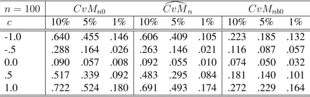
Table 1: Empirical rejection probabilities underDGP1
n = 100 CvMn0 CvM[n CvMnb0 c 10% 5% 1% 10% 5% 1% 10% 5% 1% -.3 .997 .993 .950 .998 .992 .954 .671 .621 .531 -.2 .982 .949 .792 .979 .949 .778 .516 .456 .394 -.1 .739 .617 .349 .733 .620 .348 .301 .256 .204 0.0 .104 .051 .012 .104 .055 .012 .065 .044 .032 .1 .667 .519 .256 .670 .507 .247 .278 .245 .184 .2 .961 .913 .740 .956 .907 .719 .498 .443 .371 .3 .998 .987 .928 .995 .987 .928 .671 .628 .560
Table 2 displays empirical rejection probabilities for the three tests considered under DGP2 as given above in (19). The overall picture that emerges is quali-tatively similar to that which emerges from Table 1. In particular, our proposed multiplier bootstrap-based tests exhibit more accurate empirical sizes and higher power than the conventional test based on subsampling.
Table 2: Empirical rejection probabilities underDGP2
n = 100 CvMn0 CvM[n CvMnb0 c 10% 5% 1% 10% 5% 1% 10% 5% 1% -1.0 .640 .455 .146 .606 .409 .105 .223 .185 .132 -.5 .288 .164 .026 .263 .146 .021 .116 .087 .057 0.0 .090 .057 .008 .092 .055 .010 .074 .050 .032 .5 .517 .339 .092 .483 .295 .084 .181 .140 .101 1.0 .722 .524 .180 .691 .493 .174 .272 .229 .164
The simulations presented here have indicated that our proposals for multiplier bootstrap-based tests perform favourably when compared to more conventional specification tests based on subsampling. In particular, the results presented in Tables 1–2 indicate a substantial improvement in power associated with our pro-posals when compared with a specification test based on subsampling the statistic
given above in (21). Given the popularity of subsampling for inference involving the quantile regression process,27 the results presented here suggest the possibil-ity of less computationally demanding inference methodologies for the quantile regression process involving some form of multiplier bootstrap.
6
Empirical Example: Import Substitution in the
Indian Pharmaceuticals Market
The desirability of patent enforcement on pharmaceuticals developed in high-income countries is often contentious when one considers its effect on consumer welfare in lower-income countries. This issue is bound up with the desirability of providing life-saving medicines to patients in developing countries at low cost— indeed, a typical argument made by governments of lower-income countries is that the enforcement of patents on essential medicines developed in rich countries will lead patients in poor countries to pay significantly more for these drugs than would otherwise be the case, leading in turn to adverse effects on the health and well-being of patients in lower-income countries. The other side of the debate typically involves the claim by multinational pharmaceutical firms that the enforcement of product patents is unlikely to have significant effects on prices due to the typical existence of lower-cost therapeutic substitutes for most patented drugs. A further claim is that the absence of effective patent protection in lower-income countries serves as a disincentive to basic research on diseases that have a disproportionate impact on patients in those countries. In other words, the enforcement of pharma-ceutical product patents serves as a stimulus to product innovation.
In what follows we consider the structure of demand for a particular subseg-ment of the market for systemic anti-bacterial drugs (i.e., “antibiotics”) in India. We make use of data originally analyzed by Chaudhuri et al. (2006) on sales in-volving antibiotics containing fluoroquinolone molecules. Chaudhuri et al. (2006) note that the Indian market for pharmaceutical products in the period between 1972 and 2005 provides an ideal setting for the study of the effects of global patent enforcement on consumer welfare in low-income countries. This is due on the one hand to the Indian government’s non-recognition during this period of patents on phamaceutical products and on the other hand to the existence of a large domestic pharmaceutical industry with the capacity for producing and marketing
drugs domestically that are under patent elsewhere.28 The structure of demand in the Indian market is also similar to that of many other low-income countries because of the existence of a high proportion of uninsured households that are required to meet all expenses for drugs on an out-of-pocket basis. In addition, Chaudhuri et al. (2006) observe that the Indian pharmaceuticals market is typical of that of many lower-income countries due to the disproportionate importance of anti-infective drugs, which at 23 percent is the second-largest category in terms of overall market share.29
Chaudhuri et al. (2006) analyze a dataset that consists of monthly observa-tions on sales of systemic antibiotic drugs in India over the period January 1999– December 2000.30 The data are further disaggregated by geographical region, pharmaceutical product group and national origin (i.e., Indian or non-Indian), re-sulting in a total of 672 observations. Chaudhuri et al. (2006) focus on the particu-lar market segment involving fluoroquinolone molecules, which denote a category of active pharmaceutical ingredients in treatments for a large number of different bacterial infections. 31 The fluoroquinolones segment is one of the largest in the Indian market for systemic antibiotics, accounting as it does for 20 percent of sales within this market. This segment is also characterized by the simultaneous avail-ability in India during the sample period of antibiotic treatments that are protected by United States patents as well as of generic substitutes produced by domestic firms. The existence during the sample period of several close substitutes within the fluoroquinolones segment with different countries of origin enables the empir-ical evaluation of the claim that patent enforcement on foreign drugs raises prices in the domestic market. In particular, this claim is not credible if there exist sig-nificant substitution effects between patented and nonpatented drugs containing the same active pharmaceutical ingredient.
28Chaudhuri et al. (2006) note that pharmaceutical product patents were not recognized under
Indian law between April 1972 and March 2005. They also note that the Indian pharmaceutical sector is now the world’s largest producer, by volume, of generic formulations destined to be consumed by patients.
29Anti-infectives include both antibiotic and anti-viral drugs. This category is much more
im-portant in lower-income countries than in the overall world market for pharmaceuticals. In partic-ular, anti-infectives account for only 9 percent of the worldwide market for pharmaceuticals.
30The actual dataset along with detailed information on each variable may be downloaded from
http://www.princeton.edu/˜pennykg\TRIPS_Data&Programs.zip.
6.1
The model
The empirical illustration presented here involves the estimation of a variant of the almost ideal demand system (AIDS) of Deaton and Muellbauer (1980b) involving two stages of expenditure allocation amongst categories of different pharmaceu-tical products.32 The first stage involves a model of the optimal allocation of ex-penditures to various categories of systemic anti-bacterial drugs, including those containing fluoroquinolone molecules as active pharmaceutical ingredients. The second stage involves the optimal allocation of expenditures to the various product groups within the fluoroquinolones segment. In this connection, a fluoroquinolone “product group” is taken to refer to groups of pharmaceutical formulations pro-duced by firms having the same national origin and containing the same active pharmaceutical ingredient within the fluoroquinolone category. The national ori-gin of a pharmaceutical firm is taken to be one of two types, namely “domestic” if Indian or “foreign” if non-Indian, while the active pharmaceutical ingredient refers to a specific molecule within the fluoroquinolone family. This results in seven different fluoroquinolone product groups, to wit:
1. foreign ciprofloxacin 2. foreign norfloxacin 3. foreign ofloxacin 4. domestic ciprofloxacin 5. domestic norfloxacin 6. domestic ofloxacin 7. domestic sparfloxacin
The monthly data on prices and expenditures across each of these fluoroquinolone product groups are also disaggregated by geographical region, namely, “northern”, “eastern”, “western” or “southern”.
In what follows, we focus specifically on an AIDS model for expenditure al-location amongst the first six of the seven product categories just listed. In par-ticular, we examine the extent to which Indian consumers in the period January 1999–December 2000 engaged in behaviour consistent with substitution between foreign and domestic formulations containing the same fluoroquinolone molecule.
For a given fluoroquinolone product group, let
D01 ≡
the set of all other fluoroquinolone product groups with different active pharmaceutical ingredients but
produced by firms of the same national origin
D00 ≡
the set of all other fluoroquinolone product groups with different active pharmaceutical ingredients and
produced by firms of different national origins
For a given product groupiwithin the fluoroquinolones category observed in ge-ographical regionr, let
pir ≡(pir,11, pir,10,p⊤ir,01,p⊤ir,00)⊤
be the relevant vector of prices, where
pir,11 =
{
the own price
pir,10 =
the price of the product group in the same region having the same active pharmaceutical ingredient but
produced by firms of a different national origin. Also let
pir,01 ≡ (pjr,01: j ∈D01)⊤
pir,00 ≡ (pjr,00: j ∈D00)⊤
denote subvectors of prices for product groups inD01andD00, respectively.
The basic AIDS model we consider has the form
logωirpir = τir(Uir) +γi,11(Uir) logpir,11+γi,10(Uir) logpir,10
+γi,01(Uir) ∑ j∈D01 logpjr,01+γi,00(Uir) ∑ j∈D00 logpjr,00 +βi(Uir) log ( XQr PQr ) , (22)
where ωirpir is the expenditure share for product group i in region r when the
vector of relevant prices is pir, XQr is the overall expenditure in regionron
flu-oroquinolones, and PQr is the corresponding Stone price index. Uir denotes an
![Table 3: Tests of linearity of structural quantile functions over the range [.05, .95]](https://thumb-us.123doks.com/thumbv2/123dok_us/9047023.2802594/33.918.328.592.227.382/table-tests-linearity-structural-quantile-functions-range.webp)
![Table 4: Tests for constant coefficients for quantiles over the range [.05, .95]](https://thumb-us.123doks.com/thumbv2/123dok_us/9047023.2802594/35.918.230.708.228.395/table-tests-constant-coefficients-quantiles-range.webp)

