Inflation dynamics, marginal cost, and the output gap: evidence from three countries

Inflation dynamics, marginal cost, and the output gap:

Evidence from three countries

Katharine S. Neissa,* and Edward Nelsonb,* a

Monetary Analysis, Bank of England, London EC2R 8AH, U.K. b

Monetary Policy Committee Unit, Bank of England, London EC2R 8AH, U.K.

Preliminary February 2002

Abstract

Recent studies by Galí and Gertler (1999), Galí, Gertler, and López-Salido (GGL)(2001a,

2001b), and Sbordone (1998, 2001) have argued that the New Keynesian Phillips curve (Calvo pricing model) is empirically valid, provided that real marginal cost rather than detrended output is used as the variable driving inflation. GGL (2001a) conclude that real marginal cost is not closely related to the output gap, and that models for monetary policy therefore need to include labor market rigidities. An alternative interpretation is that marginal cost and the output gap are closely related, but that the latter needs to be measured in a

manner consistent with dynamic general equilibrium models. To date, there has been little econometric investigation of this alternative interpretation. This paper provides estimates of the New Keynesian Phillips curve for the United States, the United Kingdom, and Australia using theory-based estimates of the output gap. We find little support for the notion that labor costs explain inflation dynamics better than the output gap, and so conclude that modeling of labor market rigidities is not a high priority in analyzing inflation.

* The views expressed in this paper are our own and should not be interpreted as those of the Bank of England or the Monetary Policy Committee.

Corresponding author: Edward Nelson, MPC Unit HO–3, Bank of England, Threadneedle St, London EC2R 8AH, United Kingdom. Tel: +44 20 7601 5692. Fax: +44 20 7601 3550.

1 Introduction

Recent contributions by Galí and Gertler (1999), Galí, Gertler, and López-Salido (2001a, 2001b), and Sbordone (1998, 2001) have provided empirical support for what Roberts (1995) termed the “New Keynesian Phillips curve” (NKPC). These are encouraging findings for the use of dynamic general equilibrium models in monetary policy analysis, as they suggest that the observed dynamics of inflation can be

understood with models derived from microeconomic foundations. In particular, as shown in Rotemberg (1987) and Roberts (1995), the forward-looking dynamics that underlie the New Keynesian Phillips curve emerge from optimal firm responses to obstacles to adjusting prices of the type introduced by Rotemberg (1982) and Calvo (1983). Previous work, e.g. Fuhrer (1997), had suggested that the NKPC was highly counterfactual, and that backward-looking models were required to understand empirical inflation dynamics. The recent studies suggest, however, that the NKPC does work empirically if marginal cost is used as the process driving inflation, instead of a measure of output relative to trend.

At the same time, the implications for macroeconomic modeling of recent results on the NKPC are unclear. A crucial issue is how to interpret the empirical success of NKPCs that use marginal cost as the driving process and the failure of those that use detrended output. One interpretation, in Galí and Gertler (1999) and Galí, Gertler, and López-Salido (GGL) (2001a, 2001b) for example, is that the results imply that the relationship between real marginal cost and the output gap is weak.1 According to New Keynesian models, a simple structural relationship between inflation and the output gap does not hold in general—it holds only if the labor market is perfectly competitive. If the labor market is not competitive, labor frictions become crucial. Incorporating labor market imperfections is then necessary to model the response of inflation to a monetary policy shock. The minimal number of endogenous variables needed in a realistic monetary policy analysis is then five: inflation, output, nominal interest rates, real marginal cost, and labor input (see Erceg, Henderson, and Levin (EHL), 2000, Table 1).2 In particular, one then needs to model the “wage markup” produced by monopoly power in labor supply, which drives a wedge between real marginal cost and the output gap (see e.g. GGL, 2001a). We will refer to this interpretation of the NKPC findings as the “wage markup” interpretation.

—————————————————————————————————— 1

For example, Galí and Gertler (1999, p. 204) state that a “fundamental issue, we believe, is that even if the output gap were observable the conditions under which it corresponds to marginal cost may not be satisfied.”

2

Of course, by substitution, one could reduce the number of variables in the analysis. But this may not be a straightforward procedure if there are several types of imperfection in the labor market.

An alternative interpretation, recognized but not endorsed in the above papers, is that the poor performance of detrended output-based NKPCs is not evidence against

output-gap-based NKPCs; rather, it is evidence of difficulties in measuring the output gap. Under this interpretation, real marginal cost has a closer relationship to the true output gap than do traditional, trend- or filter-derived measures of the latter. Real shocks produce fluctuations in the natural level of output, which is therefore not well approximated as smooth. This “output gap proxy” interpretation of marginal-cost-based NKPCs is endorsed, and evidence in its favor provided, by Galí (2000), Neiss and Nelson (2001), and Woodford (2001a). This interpretation implies that monetary policy analysis can be validly conducted using compact systems consisting of three variables: inflation, output, and nominal interest rates.3

Distinguishing between the “wage markup” and “output gap proxy” interpretations of the NKPC is important not only for choosing the appropriate model for monetary policy, but also the appropriate targets of policy. EHL’s (2000) analysis suggests that price inflation targeting is suboptimal in hybrid sticky price/sticky wage models; rather, central banks should target a mixture of price and nominal wage inflation. If, however, the “output gap proxy” interpretation of NKPCs is valid, then the goods market is the only source of nominal rigidity in the economy that is distorting outcomes for real variables, and price inflation targeting is optimal (Goodfriend and King, 2001; Woodford, 2001b).

In this paper, we provide evidence that the output gap proxy interpretation of the NKPC deserves reconsideration. Using data for three countries—the United States, the United Kingdom, and Australia—we find that output-gap-based NKPCs deliver correctly signed and interpretable estimates, and are competitive in fit with cost-based NKPCs, provided the potential GDP series is derived in a manner consistent with theory. To date, direct estimation of output-gap-based Phillips curves with the gap measured in a theory-consistent manner has been impeded by technical obstacles to defining and measuring potential GDP in the realistic case when potential is partly determined by endogenous state variables (such as the capital stock). The algorithm used in Neiss and Nelson (2001) overcomes these obstacles and enables us to generate a theory-consistent gap series.4

—————————————————————————————————— 3

In models with endogenous investment, consumption and the capital stock would be added to this list. 4

GGL (2001b) argue that they are able to obtain an “inefficiency gap” series from U.S. data while imposing minimal parametric assumptions, and use this series to draw inferences about empirical output gap behavior. However, as we show below, these assumptions rule out persistence in the IS equation (either from serially correlated preference shocks or from habit formation), and so the implied model of potential is more restrictive than that in the studies of Rotemberg and Woodford (1997), McCallum and Nelson (1999), Amato and Laubach (2001), Ireland (2001), and Neiss and Nelson (2001), in all of which serially correlated IS shocks are an important source of output variation.

We note two other criticisms of sticky price models addressed in this paper. First, EHL (2000, p. 298) argue that models with only nominal price rigidities cannot rationalize a disturbance (or “cost-push shock”) term in empirical NKPCs, that is the basis for the existence for a trade-off between price inflation and output gap

variability. We will argue that such a shock term can be rationalized even in the absence of labor market rigidities, once one considers the interpretation as a “price level shock” as in Meltzer (1977). Second, Christiano, Eichenbaum, and Evans (2001) argue that labor market rigidities are required to explain the sluggish response of inflation to a monetary policy shock. We contend that this sluggish response can be largely accounted for provided that the reaction of the output gap is protracted. This sluggishness, in turn, may arise largely from intrinsic dynamics in output behavior (e.g. from habit formation and capital adjustment costs).

We explore one more argument in favor of output-gap-based NKPCS. Within the confines of the current generation of models, the most one can say in favor of gap-based NKPCs is that they should perform no worse than cost-gap-based NKPCs. This is because, in these models, monetary policy only affects inflation by affecting current and prospective marginal cost. However, there are some grounds—which might be labelled “monetarist” but are also associated with James Tobin (1974)—for expecting Phillips curves with the output gap to be more robust than those with marginal cost. Under this interpretation, the aggregate demand/aggregate supply balance matters for inflation outcomes—details of input markets matter only insofar as they affect

potential output. The unit labor cost/inflation relationship, while certainly present in the data, need not be central for understanding the effects of monetary policy. And output-gap-based Phillips curves may be more reliable for analyzing changes in the steady-state inflation rate. The cost-based NKPC insists that labor share and inflation move together; in practice, however, permanent shifts in labor’s share of income do occur without shifts in steady-state inflation, and vice versa. We find that there is some empirical support for the position that gap-based NKPCs dominate marginal-cost-based NKPCs.

Our paper is organized as follows. Section 2 discusses recent empirical work on the NKPC, focussing on the contrast between “wage markup,” “output gap proxy,” and “monetarist” interpretations of this work. Section 3 gives a model of potential GDP determination used for our empirical measurement of output gaps. Section 4

describes our data and specification. In Section 5 we estimate the NKPC for the United States, the United Kingdom, and Australia, using our model-consistent output gap series. Section 6 concludes.

2 Existing estimates of the New Keynesian Phillips curve: a summary and reinterpretation

In this section we provide a brief discussion of output-gap-based and marginal-cost-based New Keynesian Phillips curves (Section 2.1); offer an interpretation that is more favorable to the output-gap-based NKPC than the existing literature (Section 2.2); and consider other reasons why output-gap-based Phillips curves might be more robust than cost-based Phillips curves (Section 2.3).

2.1 Empirical work on the NKPC: costs vs. gaps

The basic idea behind the New Keynesian Phillips curve (NKPC) is that the profit-maximizing response of firms to obstacles to adjusting prices, is to solve dynamic optimization problems. The first order conditions for optimization then imply that expected future market conditions matter for today’s pricing decisions. In aggregate, and combined with assumptions of competitive factor markets, this implies the following NKPC describing the behavior of annualized quarterly inflation (πt a):

πta = βEtπt+1a + λy(yt – yt*) + ut , (1)

where constant terms are suppressed, ytis log output, and yt* is log potential output. The parameter β corresponds to the discount factor and so should be close to one; the parameter λy is a function of the firm structure and price adjustment costs, and satisfies λy> 0. See e.g. Roberts (1995), Sbordone (1998), or Walsh (1998), for derivations. The disturbance term ut is labelled a “cost-push” shock by Clarida, Galí and Gertler (1999), although (as discussed below) we prefer the term “price level shock.” As we discuss in Section 4.4, various rationalizations of the ut term have been advanced, but for the moment we simply assume that it is exogenous in the sense that it is not proxying for omitted dynamics or excluded endogenous variables.

There have been numerous problems with empirical estimates of equation (1). While Roberts (1995) did find a positive and significant value of λy on annual U.S. data, analogous tests on quarterly data have been less favorable. GGL (2001a, p. 1251) find that instrumental variables estimates of (1) on quarterly U.S. and euro area data deliver coefficients on Etπt+1 near 1 (in keeping with the theory), but negative

coefficients on the “output gap” term. Indeed, they find this coefficient is

significantly negative (t = 3.5) for the U.S. Using quarterly U.S. data, Fuhrer (1997) finds that when both lags and leads of inflation are included in (1) instead of the single lead of π, the coefficient sum on the leads of π is near zero, again apparently

rejecting the NKPC.5 Estrella and Fuhrer (1999) estimate (1) on quarterly U.S. data for 1966–1997; they do find a positive estimate of λy, but it is highly insignificant (t = 0.4) and they emphasize the NKPC’s poor fit relative to backward-looking specifications. Importantly, as we discuss in Section 2.2, these papers uniformly use (log) GDP relative to a trend or filter as the empirical measure of the output gap, (yt – yt*). For example, Roberts (1995) and GG use quadratically detrended log GDP, while Fuhrer (1997) uses deviations of log GDP from a broken-linear trend to

measure the output gap and finds similar results when potential output is modeled as following linear, quadratic, or spline-based trends. Estrella and Fuhrer (1999) use the Congressional Budget Office (CBO) “output gap” series, which closely resembles broken-trend-based output-gap measures.

While some have interpreted the above results as rejections of the NKPC, recent work has suggested that forward-looking price-setting dynamics may be empirically

important, but that equation (1) is too restrictive a representation of this behavior. The firm optimization problem underlying the NKPC leads to the output-gap-based Phillips curve (1) only under additional conditions, notably the assumption of flexible wages. These assumptions imply that the output gap and log real marginal cost are perfectly correlated. In the more general case, equation (1) may not hold, but the firm’s optimality condition, relating its pricing decisions to the stream of current and expected future marginal costs, would continue to hold. Under conditions discussed in Sbordone (1998), this first order condition implies in aggregate the following marginal-cost-based NKPC:

πta = βEtπt+1a + λ mct+ ut (2)

where mct is the log of real marginal cost, and λ > 0. Estimates of this equation have been far more satisfactory than equation (2). For example, Galí and Gertler (GG) (1999, p. 207) obtain on 1960–1997 quarterly U.S. data an estimate of β of 0.942, and a coefficient of 0.092 (t = 1.9) on mct; and GGL (2001a, p. 1250) find on 1970–1998 quarterly euro area data estimates of β = 0.91 and λ = 0.352 (t = 2.1). These papers use instrumental variables estimates; alternative estimation techniques in Sbordone (1998, 2001) also support the marginal-cost-based NKPC. In light of these results, GGL (2001a) argue for models with forward-looking price setting combined with labor rigidities, which imply that equation (2) holds but the stricter, output-gap-based NKPC (1) does not.6

—————————————————————————————————— 5

Rudebusch (2002), using survey data for expectations, reports a somewhat higher and more significant weight on expected future inflation (0.29).

6

Recent work on wage rigidities in optimizing models includes Jeanne (1998), EHL (2000), Christiano, Eichenbaum and Evans (2001), Sbordone (2001), and Smets and Wouters (2001).

On the surface, then, the empirical evidence seems consistent with Sbordone’s (2001, p. 6) characterization that “inflation dynamics is well explained when real marginal cost is approximated by unit labor costs, but is not well modeled when marginal cost is approximated by output gap.” Yet we will argue instead that the output-gap-based Phillips curve (1) is a reasonable approximation in modeling inflation, and is not greatly inferior to equation (2) in its empirical performance. The next two subsections provide a reinterpretation of the existing evidence that is the basis for our argument.

2.2 The NKPC with the output gap reconsidered

In questioning the implications of the results reported, we focus on the fact that dynamic stochastic general equilibrium (DSGE) models define “potential output” or “the natural level of output” differently from that typically used in empirical work, and in a way that is explicitly related to the underlying real shocks in the economy. Specifically, the natural level of output in a DSGE model corresponds to the output level that would prevail if there were no nominal rigidities in the economy, i.e. if prices and wages were fully flexible.7 This definition implies two properties that distinguish it from standard gap measures, including those used by GGL, Roberts, and others in their tests of the output-gap-based Phillips curve.

First, potential output is affected by real shocks over the business cycle, and so does not follow a smooth trend as implied for example by detrended or filtered output-based measures of the output gap. Detrended potential output is not constant over the cycle in DSGE models. As Amato and Laubach (2002) put it, “In non- optimizing models, the output gap is constructed, both conceptually and empirically, as

deviations of output froma smooth trend, whereas, in optimizing models, the notion of potential output is different… [and] in general could be very volatile.” While the NKPC specification itself does arise from an optimizing model, empirical work on the NKPC has not always recognized the nature of potential output in optimizing models. Rather, as Sbordone (2001, p. 6) notes, “empirical estimates of the NKPC curve usually approximate potential output Ypt by some deterministic function of time...”

——————————————————————————————————

7

For example, Goodfriend and King (1997, p. 261) define the output gap as the percentage difference between output and “the flexible price level of output, i.e. that obtained in a noncompetitive RBC model.” Clarida, Galí, and Gertler (1999, p. 1665) define the “natural level of output” as “the level of output that would arise if wages and prices were perfectly flexible.” McCallum and Nelson (1999, p. 23) define “capacity output” as the level of output that would prevail “if there were no nominal frictions.” Woodford (2001b, p. 14) defines “the natural rate of output” as “the equilibrium level of output under price flexibility.” An early discussion is that by Obstfeld and Rogoff (1984), who define excess demand as the percentage difference between output and “flex-price equilibrium output… the equilibrium that would obtain if all prices were fully flexible” (pp. 160, 163).

Second, the issue does not boil down to disputes on how to detrend output (e.g. HP filtering vs. linear detrending).8 Rather, the issue is what phenomenon the output gap is supposed to capture. In DSGE models, the output gap captures that portion of the movement in output that can be attributed solely to the existence of nominal rigidities in the economy. Interpreted in this way, the output gap is not a measure of the

business cycle. For example, output may respond cyclically to real demand and supply shocks, but if prices are flexible, the output gap is zero, even though there is business-cycle-frequency variation in output. Similarly, there are serious limitations to judging the plausibility of an output gap series by whether it becomes negative during recessions. A recession (negative growth in actual output) is consistent with the output gap being positive, negative, or zero, depending on whether the source of the economic downturn is nominal or real, and on where output is in relation to potential at the beginning of the recession.

We found in simulations of quantitative DSGE models in Neiss and Nelson (2001) that the difference in output gap concepts is a far from trivial distinction. Rather, using our procedure (see Section 3.3 below) for obtaining the output gap in a DSGE model with habit and capital formation, and simulating the model under a policy reaction function estimated from the data, we found the output gap and detrended output had a negative correlation (−0.68), and that this result was robust to changing the specification of price adjustment, policy rule, preferences, and production. Cyclical variation in potential output was sizable. Our model was one where the output-gap-based NKPC (1) held near-exactly; yet attempts to estimate it would produce unfavorable results, if they were to follow the standard practice of measuring the gap by detrended output. On the other hand, equation (2) also holds in that model, and attempts to estimate it would be successful if real marginal cost was measured reliably. Thus an “output gap proxy” interpretation of the existing work on cost-based NKPCs is that their relative success reflects not the failure of the output-gap-based NKPC to hold in the data, but instead the fact that marginal cost is a better index of output gap fluctuations than is detrended output.

GG (1999, p. 204) express some sympathy with output-gap measurement problems as an explanation for the poor performance of detrended-output NKPCs and better performance of unit labor cost NKPCs, but ultimately conclude that it is

“problematic” whether “correcting for [output gap] measurement error alone” could account for the differences. Subsequent work in GGL (2001a, 2001b) is less

—————————————————————————————————— 8

Thus Fuhrer’s (1997) check that his rejections of the NKPC are robust to alternative procedures for detrending output would not resolve the problem of measuring potential discussed here.

favorable to the “output gap proxy” interpretation of labor cost-based NKPCs. In particular, GGL (2001a) reject the view that unit labor costs and the output gap are closely related in practice, and so view the success of their cost-based NKPC as testimony to the inadequacy of sticky-price, output-gap-based NKPCs. They therefore argue for model features that break the relation between the gap and unit labor costs (and so, between the gap and inflation). But we contend that, because existing estimates of output-gap-based NKPCs do not use a potential GDP series consistent with theory, the invalidity of the original NKPC (1) has not been firmly established.

2.3 Could output-gap-based Phillips curves be more robust?

In the marginal-cost formulation of the NKPC, the fundamental relations are the conditions linking unit labor cost to inflation. The circumstances under which the output gap will be the appropriate forcing process in the Phillips curve are limited to a special case. As discussed in (e.g.) EHL (2000) and GGL (2001a, Section 5), the output-gap-based Phillips curve emerges by substitution only in the special case of price stickiness, plus a competitive and flexible-wage labor market. The marginal-cost formulation of the Phillips curve is the more general relationship, and this is stressed by GGL (2001a) and Gagnon and Khan (2001) as an advantage of estimating Phillips curves of this type.

In short, the relationship between real marginal cost and inflation is regarded as more “structural” than the output gap/inflation relationship—it is hypothesized to prevail under different monetary policy rules and under relaxation of the assumption of no labor market rigidity, whereas the output-gap-based Phillips curve (1) does not have this policy invariance. For example, according to this view, a labor market shift such as greater labor union activity that leads to a rise in the “wage markup” and real unit labor costs should lead to a breakdown of output-gap-based Phillips curves, but not of cost-based NKPCs. And, in the marginal-cost formulation of the NKPC, a negative output gap only provides downward pressure on inflation if it also reduces current and prospective marginal cost.

By contrast, an alternative view that might loosely be called “monetarist” is that what matters fundamentally for inflation is the output gap, the balance between aggregate demand and potential output; and that this relationship is not less general than the marginal cost/inflation relationship. Put differently, output gap movements may influence inflation even if they are not associated with movements in costs. And

monetary policy actions may affect inflation not simply via their effect on current and expected labor costs. For example, Milton Friedman (1970) argued,

“I have seldom met a businessman who was not persuaded that inflation is produced by rising wages—and rising wages, in turn, by strong labor unions—and many a

nonbusinessman is of the same mind. This belief is false, yet entirely understandable. To each businessman separately, inflation comes in the form of higher costs, mostly wages; yet for all businessmen combined, higher prices produce the higher costs. What is involved is a fallacy of composition… It is easy to show that the widely held union-wage-push theory of inflation is not correct.”

This may be contrasted with Galí and Gertler’s (1999, p. 214) statement: “[I]n our model, causation runs from marginal cost [to] inflation.”

In arguing against wage-push as an explanation of inflation, Friedman stressed that observed rises in costs may be endogenous responses to excess demand (so that the output gap can still be regarded as the driving process for inflation), and also that wage increases not associated with excess demand may primarily lead to changes in relative rather than aggregate prices. To take these arguments into the present

literature, suppose that there are labor market imperfections that allow the output gap and costs to move in different directions, and produce a “wage markup.” Following GGL (2001a, p. 1261), the (log) wage markup log(µtw) is defined as the percentage markup of the real wage over the ratio of marginal utilities of leisure and consumption that would normally determine what a worker would accept as payment for its labor in a competitive labor market:

wt – pt = log(un/uc) + log(µtw) (3)

where wt – pt is the log real wage, and un and uc denote the household’s marginal (dis)utility from labor supply and consumption respectively in period t. With log real marginal cost given by mct = wt – pt−(yt−nt) (i.e., log real unit labor cost),9 the forcing process in the cost-based NKPC (2) is increasing in the wage markup:

πta = βEtπt+1a + λ[log(µtw) + log(un/uc) −(yt−nt)], (4)

so inflation is increasing in the degree of monopoly power exerted by workers.

Suppose that there is labor-union “wage-push” today that raises the wage markup, µtw, while monetary policy simultaneously keeps the output gap constant.10 According to

—————————————————————————————————— 9

The entire discussion in this paper will be in the context of models where unit labor cost and marginal cost coincide. For an examination of the empirical importance of relaxing this assumption, see

Sbordone (1998) and Gagnon and Khan (2001). 10

This implies that the term [ log(un/uc) −(yt −nt)] in equation (4) is roughly constant; see GGL (2001a,

equation (4), with current real marginal cost higher and no offsetting expected

decreases in future periods, inflation would rise. But as Gordon (1981, p. 4) observes, the “monetarist” position is instead that in the absence of monetary accommodation, “‘wage-push’ by unions... may be able to influence the unemployment rate or the distribution of income, but not the inflation rate.” Changes in labor market activity may indeed affect potential output and so the output gap for a given level of real aggregate demand; but their influence on inflation is only via their effect on the output gap, according to this view. So the response of monetary policy, which determines the output gap response, is crucial.

While we have labelled this view “monetarist,” it is also that held by James Tobin (1974, p. 228), who observed, “If the Fed were willing to starve the economy for liquidity, regardless of the consequences for real output and employment, presumably price indexes could be held down even when unit labor costs are rising… ”

Sentiments similar to Tobin’s have been expressed by policymakers too. For example, former Reserve Bank of Australia Deputy Governor Stephen Grenville stated, “Higher interest rates reduce activity and create an ‘output gap’… Inflation responds to this output gap, both directly and through the indirect effect on wages.” (Grenville, 1995, p. 209). Contrary to some New Keynesian work, these statements stress that the output gap influences inflation not just through influencing current and expected future marginal cost.

Indeed, as we now discuss, we believe that output-gap-based NKPCs may be more robust empirically than cost-based NKPCs, in the sense of being more likely to be

policy-invariant and constant in the face of changes in the economy’s structure. To see this, we note that derivations of the NKPC are typically based on a loglinear approximation around a steady state. So in principle, the inflation and unit labor cost variables that appear in the cost-based NKPC refer to stationary deviations from constant values of the steady-state inflation rate and labor share, respectively. In practice, however, Phillips curves like (2) are estimated over periods in which the steady-state inflation rate changes. GGL (2001a), for example, use the NKPC to model euro area inflation for 1970–1998, which clearly exhibits a downward trend.11 That is, GGL treat equation (2) as though it holds globally.12 To account for the downward trend in inflation, GGL rely on a downward trend in the euro area labor share. But this seems problematic on a priori grounds. There are many reasons for —————————————————————————————————— 11

See Coenen and Wieland (2000) and GGL’s (2001a) Figure 1. 12

Similarly, Ravenna (2000) simulates the NKPC to account for the early 1990s Canadian disinflation. On the other hand, Coenen and Wieland (2000) detrend their euro-area inflation series prior to

believing that changes in the structure of the economy will create changes in the steady-state labor share of income. And since labor share is a real variable, it seems unreasonable to expect that these real changes must imply changes in the steady-state inflation rate. GGL (2001a) speculate that the longer-term movements in the labor share in the 1970s and 1980s may have led to inflation because the monetary authorities accommodated the labor market changes. As theyput it,13

“steady real wage increases from the early 1970s through the early 1980s—possibly emanating from union pressures—placed consistent upward pressure on real marginal

cost. This persistent supply shock (in conjunction with accommodating European

central banks) likely played a key role in the double-digit inflation and general stagnation in Europe at this time.” (GGL, 2001a, p. 1239, emphasis added).

But if inflation only follows the labor share when monetary policy is accommodative, then the cost-based NKPC (2) is not a policy-invariant equation, and the monetarist critique of the “union-pressures” explanation of inflation, encapsulated by the Friedman and Gordon quotations above, applies.

These problems with cost-based NKPCs are less applicable to output-gap-based NKPCs. Changes in the steady state of the real economy do not imply changes in the steady state value of the output gap. Rather, if the natural rate hypothesis is

approximately satisfied, the output gap tends to zero on average.14 So if the gap-based NKPC is used to model inflation, a change in the steady state of the real economy that alters the state labor share need not lead to a prediction of a changed steady-state inflation rate. In that sense, it is more legitimate to treat equation (1) as holding globally, not just for fluctuations around a constant steady state.

So there are, we believe, some grounds for believing that output-gap-based NKPCs will be more empirically robust than marginal-cost-based NKPCs. These grounds buttress the case for re-examining output-gap-based NKPCs. But this case is already strong because the “output gap proxy” interpretation of cost-based NKPCs that we made in Section 2.2 deserves investigation. To begin this investigation, we introduce a model of potential output.

—————————————————————————————————— 13

See also GGL (2001a, fn. 17). There, however, the authors use the terms “output gap” and “capacity utilization” interchangeably. In optimizing models, there is no necessary relationship between the output gap and capacity utilization.

14

If β is less than 1.0 in equation (1), the output gap would appear to be nonzero on average if the steady-state inflation rate is constant. However, if we follow Svensson’s (2001) assumption that nominal contracts are indexed to the steady-state inflation rate, then equation (1) does imply a zero output gap when steady-state inflation is constant.

3 A model of potential output

In this section we describe a dynamic stochastic general equilibrium model, based on Neiss and Nelson (2001) that we use to obtain potential output series for estimation of output-gap-based Phillips curves in our empirical work in Section 5.

3.1 Model equilibrium conditions

We concentrate on the household side of the model, since that is from where most of the conditions that define potential output emerge. The representative household has a utility function of the form E0Σt=0∞βtu(Ct, Ct−1, 1−Nt); where Ct is its period t consumption of a Dixit-Stiglitz aggregate and Nt is the fraction of time worked in period t. Utility from money holding can be neglected in computing potential GDP. The period utility function we use is of the form u(•) = λtc(σ/σ−1)(Ct/Ct−1h)(σ−1)/σ + b(1−Nt), σ∈(0,1), b > 0. Parameter h∈[0,1) indexes the degree of habit formation. Period utility has a multiplicative disturbance, λtc, to consumption preferences—an “IS” or “real demand” shock whose effects we discuss below.

For our purposes, the key terms in the period t household budget constraint are:

Ct + (Bt+1/Pt) + Xt = wtrNt + (1 + Rt−1)Bt–ϕXt+12, (5)

where wtr is the real wage in period t,and Bt is the quantity of short-term securities (redeemed for 1+Rt−1 units of period t output) carried over from t−1 (so Rt is the short-term nominal interest rate in period t). The variable Xt, “quasi-investment,” is related to the household’s capital stock Kt by Xt = Kt+1 –(1−δ)Kt,δ∈[0,1). If there were no capital adjustment costs, Xt would correspond to investment expenditure. The size of capital adjustment costs is determined by the parameter ϕ ≥ 0.

After substituting in the first-order condition for consumption and the Fisher relation (1+Rt) = Et(1+rt)(1+[Pt+1/Pt]), three of the key first-order conditions used in our computation of potential output are those for consumption, labor supply and bond holding:

ψt= λt(Ct/Ct−1h)([σ−1]/σ)(1/Ct) –βhEtλt+1(Ct+1/Cth)([σ−1]/σ)(1/Ct) (6)

b = wtrψt (7)

where ψt is the Lagrange multiplier on the period t wealth constraint. An optimality condition for capital accumulation will also be relevant in determining potential.

On the firm side, a generic firm j∈[0,1] faces a Dixit-Stiglitz demand function for its output Yjt. It has a Cobb-Douglas production function Yjt= AtNjtαKjt1−α, where At is a technology shock, and α∈(0,1). In symmetric equilibrium, profit-maximizing choice of Njt will lead to the condition

α(Yt/Nt) = µtGwtr, (9)

as well as an analogous condition for optimal rental of capital. Here, µtG > 1 is the gross markup of price over marginal cost, present because of monopolistic

competition in the goods market.

3.2 Potential output with no capital or habit formation

As a preliminary step to obtaining an expression for potential output, it is useful to look at potential GDP behavior in a stripped-down version of the above model. This stripped-down version does not include capital or habit formation. Combining labor supply and demand conditions (7) and (9), and loglinearizing the other conditions, the result is the compact system:

yt = Etyt+1−σrt + σ(1−ρλ) λt (10)

(1−(1/σ))yt−nt –µt + λt = 0 (11)

yt = at + αnt. (12)

Here yt is log output, nt log labor input, µt the log markup, and λt the log of λtc. Logged variables should be regarded as deviations from their steady-state values (and

rt as in units of quarterly fractional deviations from its steady-state value). The “IS shock” λt has an AR(1) parameter denoted ρλ.

An important property of this small system is that λt appears as a shock term not only in the IS equation (10), but also in the labor market equilibrium condition (11). This type of IS shock—a multiplicative stochastic term in the households’ preferences over consumption, which in turn leads to a term in λt in the expression for log marginal utility of consumption—is used in the preference specifications of McCallum and Nelson (1999), Amato and Laubach (2001), Ireland (2001), Neiss and Nelson (2001), Woodford (2001b), and others. GGL (2001b) carry out an identification scheme to

obtain an estimate of the “inefficiency gap” in US data, which they use as the basis for drawing implications about U.S. output-gap behavior. GGL’s identification scheme rests on an assumption of negligible variation in any preference shock term that appears in the labor condition (11). They can then interpret any residual left over from the linear combination of yt, nt, and µt as a “wage markup” term reflecting the existence of labor market rigidity. But, because it is part of the marginal utility of consumption expression, the preference shock λt appears in our labor equilibrium condition even though the household’s preferences over leisure are nonstochastic. GGL’s identification scheme is thus quite restrictive in the sense that it rules out as a special case the preference specification of many existing quantitative sticky-price DSGE models.15 A corollary of this that these standard models do not need to rely on labor market imperfections to justify a stochastic relationship between yt, nt, and µt.

The flexible-price version of the above system corresponds to the case where yt, nt, and rt are equal to their natural values yt*, nt*, and rt*. In the class of model used here, it is the case that when output is equal to potential, the markup is constant; so µt = 0 for all t.16 The flexible-price values of real variables can then be obtained from the implied versions of equations (10)–(12), with nt* removed by substitution:17

yt* = Etyt+1* −σrt* + σ(1−ρλ) λt (13)

(1−(1/σ)−(1/α))yt* + (1/α)at + λt = 0. (14)

The minimal-state-variable solutions for both (the log of) potential output yt* and the natural real interest rate can be expressed in terms of productivity and real demand shocks:

yt* = π1at + π2λt (15)

rt* = π3at + π4λt, (16)

—————————————————————————————————— 15

It might be thought that an IS shock term in (10) could be retained and that in (11) removed by assuming, as in Rotemberg and Woodford (1997), that the preference shock is part of the household’s discount factor rather than a multiplicative term in the period utility function. But this alternative assumption would imply a stochastic discount factor ({βt}t=0 ∞ instead of {βt}t=0 ∞) in the NKPC (2). The validity of GG’s and GGL’s use of lagged variables as instruments in their estimation of the NKPC rests on any shock to the discount factor being white noise. So GGL’s (2001b) procedure for making inferences about U.S. output-gap behavior does depend on the assumption that serially correlated preference shocks are unimportant over the cycle.

16 _{This is because under Dixit-Stiglitz monopolistic competition, the optimal markup of prices over} costs is constant under price flexibility. Then real marginal cost, which is the inverse of this markup, is also constant.

17

Examination of eqs. (11) and (14) verifies that the output gap/real marginal cost relationship stressed by GG (1999) holds in this model. Substituting (12) into (11) and expressing relative to (14), we have:

(1−(1/σ)−(1/α))(yt – yt*)–µt = 0.

where the πi coefficients can be obtained by substituting these expressions into (13)– (14) and applying the method of undetermined coefficients. The implied values for the πi are:

π1 = 1/(1−α+[α/σ]) > 0, (17)

π2 = σ/(1−σ +[σ/α]) > 0, (18)

π3 = −π1([1−ρa]/σ) < 0, (19)

π4 = (1−ρλ)(π2−σ)/σ > 0. (20)

Here, ρa denotes the AR(1) parameter driving the productivity shock. These expressions illustrate that potential output and the natural real interest rate in the above model respond to temporary shocks to both productivity and real demand. Productivity shocks raise potential output but reduce the natural interest rate, while real demand shocks raise both potential output and the natural rate.

This simple case highlights several important properties of the model-derived concept of the output gap that carry over to more general environments. First, potential output is a function of both supply and real demand shocks. Describing fluctuations in potential output as arising solely from “aggregate supply shocks” should, in general, be regarded only as shorthand.18 Second, since the potential output series defined in equation (15) pertains to the deviation of potential output from trend, it immediately follows that, as noted in Section 2, detrended potential GDP is not constant over the cycle. This renders invalid not only trend-based approaches to measuring the output gap, but also standard “production function approaches” to measuring the output gap (such as the CBO output gap series in Estrella and Fuhrer, 1999). Production function approaches fail to address fully the aspects of potential output behavior stressed here. They typically recognize changes in the full-employment labor force due to

demographic and labor market developments.19 But potential GDP can vary cyclically in a dynamic general equilibrium model even if the economy’s demographic

characteristics are unchanged. For example, government spending shocks, terms of trade shocks, tax changes, and (as here) taste shocks all affect households’ decisions regarding the timing and magnitude of consumption, and so produce variations in labor supply and potential output. Production function approaches typically neglect the effect of real shocks on the dynamics of input supplies and so on short-run potential output dynamics.

—————————————————————————————————— 18

For example, while Rotemberg and Woodford (1997, p. 316), describe their potential output series as consisting of “exogenous supply disturbances,” this labelling is a shorthand to denote all the real shocks, both demand and supply, that affect potential GDP in their model.

19

They also may allow for changes in the economy’s potential growth rate, due to the feedback from investment in physical capital to productivity growth.

3.3 Potential output with endogenous state variables

With habit formation (h > 0), the previous period’s consumption level becomes a state variable. And with capital formation present, the capital stock also enters the state vector. We denote the flexible price values of lagged log consumption and log capital by ct−1* and kt*. The resulting expression for yt* is:

yt* = π11at + π12λt + π13ct−1* + π14kt*, (21)

where the πij are solution coefficients. The solution for potential output can no longer be written as an exact, finite distributed lag of the two real shocks. But since the solutions for ct* and kt+1* are themselves linear functions of the same state vector,

repeated substitution allows (21) to be expressed as:

yt* = f(at, at−1, at−2, …, λt , λt−1, λt−2, …), (22)

and model simulations can establish how many lags of at and λt are required to obtain an accurate finite-lag approximation of the infinite-distributed lag solution given by (22). That is the procedure we use to obtain expressions for potential GDP and the natural interest rate in Neiss and Nelson (2001), and that we use in this paper to obtain empirical, model-based estimates of the output gap.

Note also that in (22) the effects of real shocks on potential GDP are spread over time, as potential output evolves in response to the real shock. The response of output under sticky prices—which we refer to as “actual” output—to real and monetary shocks will also tend to be spread over time, depending on the richness of the model. Since, according to the NKPC, inflation depends on the stream of current and

expected output gaps, persistence in the gap stream, due to the dynamics of potential GDP, may help in explain the observed persistence in inflation.20

Galí (2000), Woodford (2001a), and Neiss and Nelson (2001) provide evidence that the output gap and detrended output are not closely related. Galí (2000) and

Woodford (2001) plot real marginal cost against traditional detrended-output-based measures of the output gap, as evidence that, in the words of Galí (2000, p. 2), “the output gap… for the postwar U.S. shows little resemblance with traditional output gap measures.” In Neiss and Nelson (2001) we also argued that the output gap and

—————————————————————————————————— 20

By contrast, GGL (2001a, pp. 1242–1243) conclude, “Overall, the output-gap based formulation of the new Phillips curve cannot account for the persistence of inflation either for the U.S. or for the euro area.”

detrended output were negatively correlated, doing so not on the basis of the marginal cost profile but on evidence from simulations of a sticky-price dynamic general equilibrium model, using equation (22) to generate the potential output and output-gap series under conditions of habit and capital formation. In that model, marginal cost and the output gap have a near-exact relation, but simulations established that detrended output and the output gap were negatively related. Galí’s and Woodford’s evidence is subject to the criticism that it is equally consistent with the “wage

markup” interpretation of estimated NKPCs, and hence does not establish that

detrended output and the output gap are closely related. Our previous work is subject to the criticism that it was based on simulated data and did not attempt to generate model-consistent output gap series from data from actual economies. We undertake that exercise in this paper, and so provide direct empirical evidence for the “output gap proxy” interpretation of Phillips curves.

3.4 Completing the model of potential

To complete the model of potential GDP implied by our model, we report the first-order conditions for the households’ choices of the capital stock for period t+1:

ψt(1+2φXt) −βEtψt+1[(1−δ)(1+2φXt+1) + zt+1] = 0, (23)

where zt is the factor price for capital. An expression for potential output in terms of underlying exogenous shocks, as in equation (22), emerges from solving a log-linear system whose key equations include approximations of equations (6)−(9) and (23).

4 Data and specification

We will estimate equation (1), the output-gap-based NKPC, for three countries. Here we describe our measurement and interpretation of the three variables in equation (1): annualized inflation πta, the output gap (yt − yt*), and the shock ut. We also describe the labor share data that we use to estimate the cost-based NKPC (2).

4.1 Inflation series

While we will report results for GDP deflator inflation for the United Kingdom and the United States, the consumer price index (CPI) is our baseline series for calculation of inflation rates in the three countries in our sample. CPI inflation, unlike GDP deflator inflation, corresponds to that actually targeted by central banks and so is of greatest concern for monetary policy. It is also of interest, as in GG (1999, p. 206), to see how the NKPC performs in describing “a standard broad measure of inflation.” CPI inflation has been used for this purpose by Roberts (1995, 2001) and Estrella and Fuhrer (1999).

Another important reason for our choice is that the use of GDP deflator rather than CPI inflation in estimating the NKPC may understate the importance of the output gap for aggregate inflation outcomes. For example, part of Friedman’s (1970)

argument against wage-push theories of inflation relies on substitution effects: higher costs and prices in some sectors of the economy will, if not accommodated by

monetary policy, leave households with less to spend on goods in other sectors, producing excess supply in those sectors and thus downward pressure on prices and costs. Consider a wage-push driven increase in unit labor costs in an open economy. Even if unit labor cost increases are passed through to domestically produced goods prices, a monetary policy that restrains the output gap could lead to offsetting pressure on import prices, provided, as seems likely, import prices are set partly in response to domestic demand conditions. The lack of monetary accommodation translates labor cost changes into relative price changes rather than aggregate price level changes. A broad aggregate such as the CPI is needed to internalize these substitution effects.

An alternative view is that closed-economy NKPCs should not be used to analyze CPI inflation. On this view, import prices behave dissimilarly from other elements of the CPI and are largely associated with exchange rate and world price changes, leading to a strong influence on the CPI from open-economy factors. But this view does not have much support in the data (e.g. Stock and Watson, 2001), even for highly open

economies like the U.K., and so we proceed with an analysis that does not have explicit open-economy elements.

4.2 Labor share data

The precise definition of the labor share data used is important. Staiger, Stock, and Watson (2001) note that whether the U.S. labor share is stationary or trending

depends on the price series used to deflate nominal wages; while Batini, Jackson, and Nickell (2000) and Balakrishnan and López-Salido (2001) show for the U.K. that the significance of the labor share in NKPC estimates depends on the precise wage series used.

For the U.S., following GG, GGL and Sbordone, we use nonfarm business sector data, obtained from the BLS website. For the U.K., unit labor cost data are an updated version of the labor share data in Batini, Jackson, and Nickell (2000).

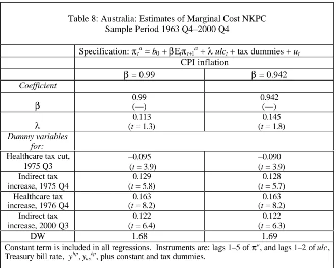
For Australia, nonfarm employment and nominal wage data are updated versions of the data used by Gruen, Pagan, and Thompson (1999).21 The product of these series was expressed as a ratio to nominal GDP and logged to produce a ulc series (ulc = (w

− pgdp−(y − n)), where pgdp is the log GDP deflator). To check robustness of results to the precise labor share definition, we also present results using two other series. The first alternative is a labor share series, ulccpi, obtained by deflating nominal wages by the CPI rather than the GDP deflator: ulccpi = (w − pcpi) −(y − n). The second

alternative is an official quarterly series on nonfarm wages’ share of nonfarm GDP, published by the Australian Bureau of Statistics.

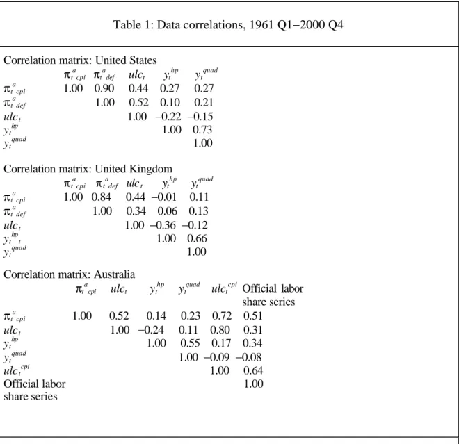
Data plots and correlations: Figures 1–3 plot labor share against quarterly annualized CPI inflation for the three countries, while contemporaneous correlation matrices for 1961 Q1–2000 Q4 are given in Table 1. The correlations refer to CPI inflation (πt

a cpi),

GDP deflator inflation (πt a

def), log real unit labor costs (labor share) (ulct), HP-filtered log output (yt

hp

), and quadratically detrended log output (yt quad

). The latter two series are, of course, frequently labelled the “output gap.” Inflation rates are defined as the annualized quarterly percentage change in the relevant price index. Only the CPI inflation rate is used for Australia because the GDP deflator inflation series, especially before 1980, is dominated by swings in export prices.

—————————————————————————————————— 21

For the U.K., while both inflation measures are positively correlated with unit labor costs, the relation is noticeably stronger for CPI inflation. This may appear surprising from the perspective of models that stress domestic-goods inflation as being driven by marginal cost, and import price inflation as determined by a different set of factors. But we have argued that there are grounds for regarding import price inflation, and so total CPI inflation, as driven heavily by domestic-economy factors.

Unit labor cost is negatively correlated with measures of detrended output in five out of six cases. For example, the correlation between HP filtered log GDP and real unit labor cost is −0.36 for the United Kingdom, −0.24 for Australia, and –0.22 for the United States. We have argued that this is indirect evidence that detrended output is a poor proxy for the output gap—not that marginal cost and the output gap are poorly related in reality. We provide evidence on this in Section 5.

Regardless of detrending method, detrended output it is quite weakly correlated with contemporaneous inflation in all three countries; the correlation is always below 0.3. This partly reflects the fact that output tends to lead inflation; allowing for this delivers Corr(πtacpi, yt−6quad) = 0.50 for the U.S., Corr(πtacpi, yt−8quad) = 0.49 for the

U.K., and Corr(πtacpi, yt−6quad) = 0.41 for Australia. But it is a harbinger of the poor

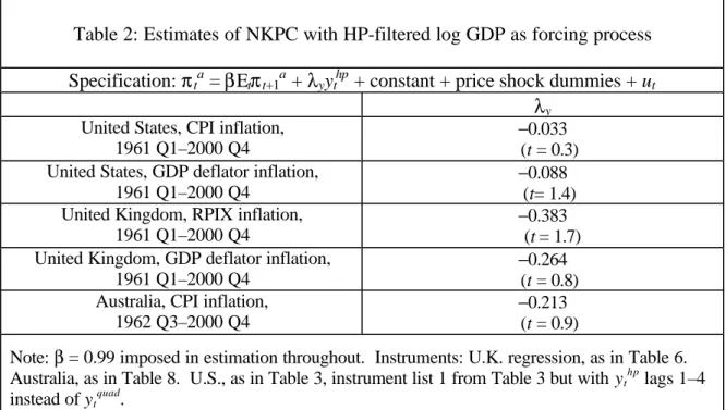
performance that NKPCs estimated with detrended output for all three countries. GG (1999, p. 201) report that the detrended-output NKPC delivers an incorrect sign on U.S. data, and GGL (2001a) report the same for the euro area. They attribute these weak results to the fact that the output-gap-based NKPC specifies inflation as a function of current and expected future gaps, while empirically, detrended output leads inflation. It follows that NKPCs with detrended output as the forcing process will not work. For our own dataset, we reaffirm this finding in Table 2. It shows that negative coefficients in detrended-output-based NKPC estimates hold regardless of inflation definition for the U.S., the U.K., and Australia.

4.3 Potential output and output gap series

We generate a theory-consistent potential GDP series for each country by calibrating key preference and production parameters, generating the implied IS and technology shocks from the data, and using the method of Section 3.3 to express potential GDP as a distributed lag of these shocks. We give a brief description here; the Appendix provides details.

The key production function parameters are set as follows: α = 0.7, δ = 0.025. These parameter choices are sufficient to generate a Solow residual from each country’s

output and factor input data. The technology shock is defined as the HP-filtered values of these Solow residuals.

For preferences, we restrict ourselves to the case where the IS shock is white noise, so that habit formation is the only source of persistence in consumption behavior. We fix the habit formation parameter h for each country to h = 0.8, Fuhrer’s (2000) estimate. We then calibrate σ, the intertemporal elasticity of substitution of

consumption, to a value consistent with λt in (6) being white noise for each country. This gives σ = 0.7 for the U.S., σ = 0.9 for the U.K., and σ = 0.6 for Australia.22 We obtain potential GDP series by solving the model of Section 3 under price flexibility and obtaining expression (22). We solve the model under two settings: (i) the basic RBC-style model without capital adjustment costs (ϕ = 0 in equation (5)); and (ii) the model with capital adjustment costs (specifically, ϕ = 0.35). Each setting implies different profiles for potential GDP. For example, the relative importance of IS shocks increases when there are capital adjustment costs, because it becomes less easy to switch the composition of a given amount of potential GDP between

consumption and investment (see our 2001 paper).

Each version of the model needs to be solved separately for each country because the countries differ in their value of σ as well as ρa, the AR(1) parameter for the

technology shocks. The “output gap” is then defined as HP-filtered GDP minus our potential GDP series.23

Figures 4–6 plot the resulting output gap series, under the assumption of capital adjustment costs, for each country against a more standard measure of the output gap—quadratically detrended output. We note three properties of the gap series. First, in contrast to GGL (2001b), we find that the theory-based output gap and detrended output are not very closely related.24 Second, the output-gap series are of much smaller amplitude than detrended output, a result consistent with our simulation evidence in Neiss and Nelson (2001) and with the hypothesis that much observed GDP variation reflects variation in potential GDP. Third, the theory-based output gap tends to lag detrended output. Mechanically, this arises from the fact that potential output is a function of lagged shocks, so the output gap tends to be more inertial than —————————————————————————————————— 22

We also set β = 0.99 in equation (6). 23

No detrending is necessary for our potential GDP series; as our estimates of the underlying real shocks that appear in equation (22) are generated from detrended or growth-rate data, our series for yt*

corresponds conceptually to the detrended level of natural GDP. 24

GGL (2001b, Table 1) find that their “inefficiency gap” series, which they use as the basis for drawing implications about U.S. output gap behavior, has a correlation with detrended output of 0.81.

detrended output. The figures therefore answer a criticism of the gap-based NKPC by GG (1999, pp. 198, 201–202, 204). They noted that the gap-based NKPC implies inflation leads the gap, and questioned whether this is consistent with detrended output leading inflation. We suggest that the two observations are not irreconcilable, because the gap itself lags detrended output.

4.4 Rationalization of the disturbance term ut

In our estimates of equations (1) and (2), we will include the disturbance term ut, i.e., a structural shock to the Phillips curve. Such a shock is needed both for realistic empirical work with these equations and to provide some trade-off between output-gap and inflation variability in (1). EHL (2000, p. 298) argue that this term is itself evidence against sticky-price models, on the grounds that models without wage rigidities cannot provide a microeconomic foundation for the presence of this term.

We argue, however, that in the case where ut is white noise, this disturbance does have an interpretation in sticky-price models, namely as a price level shock. By this we mean a shock that permanently raises the price level, but (provided that monetary policy is non-accommodative)25 only temporarily increases inflation by raising πt relative to Etπt+1a. As Meltzer (1977, p. 183) puts it,

“a one-time change in tastes, the degree of monopoly, or other real variables changes the price level… [W]e require a theory that distinguishes between once-and-for-all price changes and maintained rates of price change.”

Thus, changes in the real steady state of the economy arising from (e.g.) changes in the degree of competition, produce movements in the steady-state level of natural output. For a given measure of actual output yt, these changes in the steady state value of potential yt* should produce an output gap. A correct measure of the output gap that included variations in potential GDP due to high-frequency changes in the economy’s steady state, would capture the effects Meltzer mentions. In practice, however, the coefficients in our potential GDP expression (22) are based on the assumption of a constant steady state. In general, the log-level of (detrended) log potential output in period t is composed of a steady-state component, plus technology and IS shocks that drive fluctuations around the steady state:

yt* = mt(yt*) + b(L)at + c(L)λt , (24)

—————————————————————————————————— 25

where mt(yt*) is the steady state log-level of potential, and the b(L) and c(L) are lag polynomials. If the steady state of the economy was constant, then mt(yt*) would be a constant and the atand λt shocks then fully index the variation in potential GDP. Suppose, however, that the degree of monopoly power in the economy underwent a discrete change during the sample period under consideration.26 Then treating mt(yt*) as a constant would only be an approximation, and while there would be no mean

error in measuring yt*, there would be some variation in yt* not captured by the demand and supply shocks alone. Equation (1) can then be written:

πta = βEtπt+1a + λy(yt – yts*) −λymy,t , (25)

where yts* is the portion of potential output variation due to the shocks, and my,t =

mt(yt*) – E[mt(yt*)] is the deviation of steady state log potential in period t from a constant. Clearly, with ut≡−λymy,t, price level shocks that move steady-state

potential provide a rationale for a disturbance term in the output-gap-based NKPC (1). Furthermore, if these changes in the steady state of the economy were discrete in nature, they would provide a rationale for ut being approximately white noise.

5 Empirical results

This section presents our NKPC estimates for the three countries. We first report marginal-cost-based NKPCs analogous to those in GG, and then estimate NKPCs using a theory-based output-gap series. We begin with the United States.

5.1 United States

We first report estimates for the U.S. of the following version of equation (2):

πta = βEtπt+1a + λ ulct+ d0 + d1DNIXONt + ut . (26)

—————————————————————————————————— 26 _{Giannoni (2000) and Woodford (2001b) argue that time-varying distortions such as a changing} degree of monopoly power can create movements in potential GDP. In general, because they affect the structure of the economy, movements in these distortions affect both the steady-state level of potential (our mt(yt*) variable ) and the dynamic response of potential to shocks (the b(L) and c(L) coefficients in

equation (24)). Our price-level-shock definition is restricted to refer only to the first source of change. An increase in the steady-state markup, or an increase in the factor of proportionality in the utility function (Meltzer’s “one-time change in tastes,” which does not fall into the category of a changing distortion) would be suitable candidates as price level shocks, as they affect the steady-state potential level but not the shock response coefficients in the equilibrium expression for potential. Note that, in contrast to Giannoni, our price-level-shock interpretation of the ut process implies that the (y − y*) term

in equation (25) is still the log-deviation of output from its natural level, rather than from its efficient level.

Here DNIXONt is a dummy variable for the Nixon price controls; this follows work on backward-looking Phillips curves (Gordon, 1982) and is consistent with our wish to control for price level shocks. To capture the fact that the controls suppressed a growing amount of inflation (because monetary policy was relaxed with the controls’ introduction), we make the dummy equal to the length of time in which the controls have been in effect. The dummy is constructed on the assumption that all the suppressed inflation was recorded in actual inflation once the controls were lifted.27

GG (1999) and GGL (2001a) obtained β estimates in the 0.9–0.95 range, somewhat lower than the value of about 0.99 suggested by theory. Our own estimates of β were occasionally above 1.0 for some countries and specifications, so we report results conditional on two imposed β values: β = 0.99 and β = 0.942 (GG’s (1999) estimate).

Estimates of equation (25), first using GDP deflator inflation, are given in Table 3. Using an instrument list like GG’s,28 we obtain (for β = 0.942) a t-value of 1.4 on ulc, and a coefficient larger and more significant than reported in Rudd and Whelan’s (2001) replication, but not as significant as that (t = 1.9) reported by GG for 1961 Q1– 1997 Q4. We found, however, that modest changes in the instrument definitions and an instrument-choice strategy close to that of GGL (2001a) gave somewhat more significant results. Specifically, GGL set the lag length for instruments other than inflation somewhat shorter than for lagged inflation, the rationale being that the extra lags of inflation contribute heavily to the explanatory power of the “first-stage” regressions that underlie the instrumental variables estimates. In light of this, we formulate an “instrument set 2” that shortens the lag length of non-inflation

instruments from 4 to 2. We also replace lags of the long bond/funds rate spread as an instrument with separate lags of the Treasury bill rate and the long bond rate; replace quarterly wage and commodity inflation by the corresponding four-quarter inflation rates; and drop detrended output as an instrument.

With this different instrument set we obtain (setting β = 0.942) an estimate of λ = 0.098 with t = 1.9, similar to GG’s λ = 0.092 (t = 1.9). With CPI inflation we obtain a larger coefficient estimate and the same level of significance. When β = 0.99, which corresponds more closely to the β value suggested by theory, the size and significance of the λ estimates diminish in all cases. The Nixon controls dummy coefficient is the right sign throughout, but only contributes minor explanatory power to CPI inflation. For the GDP deflator it is highly insignificant and we drop it from the specification. —————————————————————————————————— 27

The Nixon dummy equals 1 in 1971 Q3, 4 in 1971 Q4, …, 31 in 1974 Q1, and –31 in 1974 Q2. 28

The differences are our inclusion of the Nixon dummy variable and our use of the percentage change rather than the log change in computing growth rates.

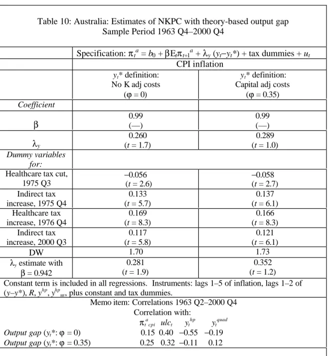
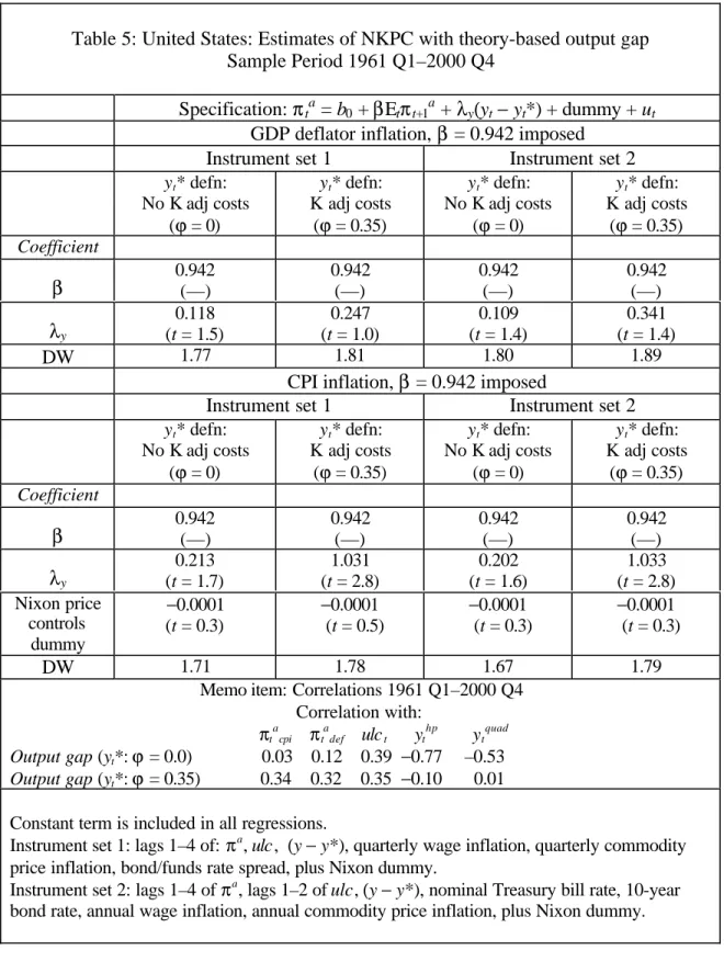
Tables 4 and 5 give NKPC estimates using our theory-based output gap as the forcing process.29 In contrast to Table 2 where the output gap was measured by detrended output, the theory-consistent output gaps enter the estimated NKPCs positively. Moreover, when CPI inflation is used and potential output is defined as subject to capital adjustment costs, the coefficients are significant (whether β = 0.942 or 0.99 is used). Indeed, in these cases our gap measure performs better in explaining inflation than did unit labor costs—consistent with the “monetarist” hypothesis regarding Phillips curves. The correlations at the bottom of Table 5 indicate that our gap measures are positively correlated with unit labor cost measures, consistent with the prediction one would make if prices were sticky and labor markets could be

approximated as competitive. One unsatisfactory aspect of the results in Tables 5 and 6, however, is that the coefficients on the output gap seem to be on the high side. In Rotemberg and Woodford (1997), for example, λy is only 0.11.30 The counterpart of their λy estimate is high output gap volatility: large gap movements lead to only modest movements in inflation. In our U.S. results, output gap variability is mild, but the inflation response to gap movements is quite strong.

5.2 United Kingdom

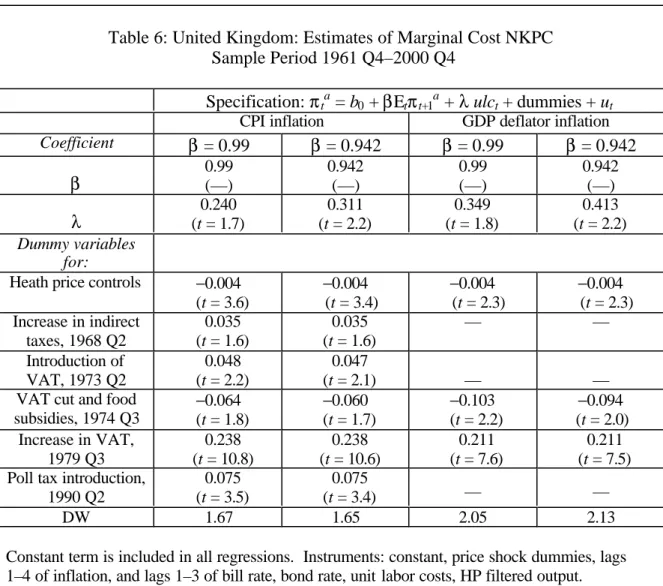
We turn next to the U.K. As for the U.S., we first report NKPC estimates with real marginal cost as the driving process. Compared to previous estimates of marginal-cost-based NKPCs on U.K. data (e.g. Amato and Gerlach, 2000; Batini, Jackson, and Nickell, 2000; Balakrishnan and López-Salido, 2001) we (i) estimate equations on broader definitions of inflation, (ii) allow explicitly for price level shocks, and (iii) estimate on a longer sample (40 years of quarterly data).

While the utdisturbance term in equation (2) accounts for price level shocks of a normal magnitude, we include dummy variables for some specific large price level increases. We include a dummy for the Heath government’s price controls of 1972– 1974. Like the Nixon controls, these were imposed alongside increasingly

expansionary monetary policy, so we define the Heath price controls as equal to the number of months that the controls have been in effect. We also include dummy variables for the increases in indirect tax in 1968, 1973 and 1979, and the 1974 cut. In principle, indirect tax (from 1973, VAT) changes are relevant primarily for CPI —————————————————————————————————— 29

As the model underlying our potential GDP series has capital and habit formation, the NKPC (1) holds only approximately (see Amato and Laubach, 2001, for the NKPC in a model with habit formation but no capital). Model simulations suggest, however, that the approximation is reasonable. 30

The estimates in Tables 5 and 6 nevertheless strongly support sticky prices over flexible prices, which correspond to the limiting case of λy infinite. Sbordone (1998) observes that even modest