Stochastic expected utility theory

Stochastic expected utility theory

Pavlo R. Blavatskyy

Published online: 19 May 2007

#Springer Science + Business Media, LLC 2007

Abstract This paper proposes a new decision theory of how individuals make random errors when they compute the expected utility of risky lotteries. When dis-torted by errors, the expected utility of a lottery never exceeds (falls below) the utility of the highest (lowest) outcome. This assumption implies that errors are likely to overvalue (undervalue) lotteries with expected utility close to the utility of the lowest (highest) outcome. Proposed theory explains many stylized empirical facts such as the fourfold pattern of risk attitudes, common consequence effect (Allais paradox), common ratio effect and violations of betweenness. Theory fits the data from ten well-known experimental studies at least as well as cumulative prospect theory.

Keywords Decision theory . Stochastic utility . Expected utility theory . Cumulative prospect theory

JEL Classification C91 . D81

Perhaps we should now spend some time on thinking about the noise, rather than about even more alternatives to EU?

—Hey and Orme (1994),Econometrica62, p.1322 This paper proposes a new decision theory to describe individual decision making under risk, as defined by Knight (1921). A normative theory of choice under risk is expected utility theory, or EUT. However, persistent violations of EUT, such as the Allais paradox (Allais1953), make EUT a descriptively inadequate theory (Camerer

1995). Many theories have been proposed to improve the descriptive fit of EUT (see Starmer (2000) for a recent review). EUT and nearly all non-expected utility theories P. R. Blavatskyy (*)

Institute for Empirical Research in Economics, University of Zurich, Winterthurerstrasse 30, 8006 Zurich, Switzerland

are deterministic theories i.e. they predict that an individual always makes the same decision in identical choice situations (unless he or she is exactly indifferent between lotteries). In contrast, this paper proposes a stochastic decision theory to explain the violations of EUT through the role of random errors. The new model is motivated both by a recent revival of interest among economic theorists in stochastic decision theories (Loomes et al.2002) and by the compelling empirical evidence of random variation in individuals’decisions (Ballinger and Wilcox1997).

For example, Camerer (1989, p.81) reports that 31.6% of the subjects reverse their preference, when presented with the same choice decision for the second time. Starmer and Sugden (1989) find that the observed preferences are reversed in 26.5% of cases. Wu (1994, p.50) reports that the revealed preferences change in 5–45% of cases when the same binary choice problem is repeated. Hey and Orme (1994) find that around 25% of choice decisions are inconsistent, when an individual faces the same choice problem twice and he or she can declare indifference. Moreover, Hey (2001) provides experimental evidence that the variability of the subjects’responses is generally higher than the difference in the predictive error of various deterministic decision theories. Thus, a model predicting stochastic choice patterns can be a promising alternative to the deterministic non-expected utility theories.

Existing non-expected utility theories typically do not consider stochastic choice patterns (see, however, Machina1985, and Hey and Carbone1995). Only when the theoretical model is estimated are assumptions about error specification introduced. Effectively, the stochastic component plays only a secondary role being regarded as unimportant on the theoretical level (Hey 2005). Camerer and Ho (1994) use a stochastic choice model in which the probability of choosing one lottery over another is simply a logit function of the difference in their utilities according to the deterministic underlying theory. Harless and Camerer (1994) assume that there is a constant probability with which an individual reverses his or her deterministic choice pattern. This probability is the same in all choice problems and it reflects the possibility of errors such as pure trembles. Hey and Orme (1994) obtain a stochastic choice pattern by means of a white noise (normally distributed zero-mean error term) additive on the utility scale. Such an error term reflects the average of various genuine errors that might obscure a deterministic choice pattern. Hey (1995) and Buschena and Zilberman (2000) go one step further and assume that this error term is heteroskedastic. The standard deviation of errors is higher in certain decision problems e.g. when the lotteries have many outcomes or when the subjects take more time to make a decision.

This paper proposes a new and more elaborate structure of an error term. The stochastic component is introduced as a part of the decision theory, which makes explicit prediction in the form of a stochastic choice pattern. Thus, econometric estimation of the proposed theory on the empirical data does not require any additional assumptions about error specification. Moreover, new theory assumes that individuals have a preference relation on the set of risky lotteries, which admits expected utility representation. Thus, the proposed theory is essentially a stochastic extension of neoclassical expected utility theory, so that its estimation is relatively simple compared to non-expected utility models.

Individuals are assumed to maximize their expected utility when choosing between risky lotteries. However, individuals make random errors when computing

the expected utility of a lottery. The errors are additive on the utility scale, as with Hey and Orme (1994). The distribution of random errors is essentially symmetric around zero with a restriction that the stochastic utility of a lottery cannot be lower (higher) than the utility of the lowest (highest) possible outcome for certain. This assumption reflects a rather obvious fact that there is a limit to a measurement error that an individual can commit. In particular, violations of obvious dominance, when a risky lottery is chosen over its highest possible outcome for sure, or when it is not chosen over its lowest possible outcome for sure, appear to be implausible. Hence, computational errors are naturally truncated by the highest and the lowest outcomes in the gamble.

This restriction implies that lotteries whose expected utility is close to the utility of the lowest possible outcome (e.g. unlikely gains or probable losses) are more likely to be overvalued rather than undervalued by random errors. Similarly, lotteries whose expected utility is close to the utility of the highest possible outcome (e.g. probable gains or unlikely losses) are likely to be undervalued by random errors. This offers an immediate explanation for the fourfold pattern of risk attitudes—a risk seeking behavior in face of unlikely gains or probable losses and a risk averse behavior in face of probable gains or unlikely losses (Tversky and Kahneman1992). A stochastic version of expected utility theory can also explain other empirical anomalies such as the common consequence effect and the Allais paradox (Allais1953), the common ratio effect and violations of betweenness (Camerer and Ho1994).

Apart from demonstrating that many empirical paradoxes can be attributed to a simple stochastic version of expected utility theory, this paper also reexamines the data from ten well-known experimental studies. The proposed theory accommodates the experimental data with remarkable success. It fits the data at least as well as such prominent non-expected utility models as cumulative prospect theory or rank-dependent expected utility theory. This suggests that a careful specification of the stochastic structure of the errors that subjects make in the experiments is a promising avenue for constructing a descriptive decision theory. Systematic errors that subjects commit when evaluating the expected utility of risky lotteries can account for many of the well-known empirical anomalies, which have been traditionally attributed to non-linear probability weighting, regret or disappointment aversion etc.

The remainder of this paper is organized as follows. Stochastic expected utility theory or StEUT is described in Section 1. Section 2 demonstrates how StEUT explains many stylized empirical facts such as the fourfold pattern of risk attitudes and the Allais paradox. Section3tests the explanatory power of StEUT on the data from ten well-known experimental studies. Section4 concludes.

1 Theory

NotationL(x1,p1;...xn,pn) denotes lotteryLdelivering a monetary outcome xiwith probabilitypi,i∈{1,...,n}. Let x1be the lowest possible outcome and let xn be the highest possible outcome. The expected utility of lotteryLaccording to deterministic preferences of an individual is m_L¼Pn_i¼1piu xð Þi . A subjective non-decreasing utility functionu:R→Ris defined over changes in wealth rather than absolute wealth levels, as proposed by Markowitz (1952) and later advocated by Kahneman and

Tversky (1979). An individual makes random errors when calculating the expected utilityμLof a risky lottery.1

Random errors are assumed to be additive on the utility scale, similar to Hey and Orme (1994, p.1301) and Gonzalez and Wu (1999). Thus, instead of maximizing deterministic expected utility μL, an individual behaves as if he or she maximizes

stochastic expected utility

U Lð Þ ¼m_Lþx_L: ð1Þ

For simplicity it is assumed that an error termxLis independently distributed across lotteries. In other words, the error which occurs when an individual calculates the expected utility of one lottery is not correlated with an error when calculating the expected utility of another lottery.

The stochastic expected utility (1) of a lottery is assumed to be bounded from below and above. It cannot be less than the utility of the lowest possible outcome for certain (see, however, Gneezy et al.2006). Similarly, it cannot exceed the utility of the highest possible outcome for certain. Formally, the internality axiom holds i.e.

u xð Þ 1 μLþxLu xð Þn , which imposes the following restriction on the cumulative distribution functionΨLð Þ ¼v probðxLvÞof a random error xL:

ΨLð Þ ¼v 0; 8v<u xð Þ 1 μL and ΨLð Þ ¼v 1; 8vu xð Þ n μL: ð2Þ Assumption (2) implies that there is no error in choice between “sure things.” A degenerate lottery delivers one outcome for certain, which is simultaneously its lowest possible and its highest possible outcome (x1=xn). In this case, Eq. (2) immediately implies that prob(xL=0)=1 i.e. the utility of a degenerate lottery is not affected by random errors.

For non-degenerate lotteries, the random errors are assumed to be symmetrically distributed around zero as long as restriction (2) is not violated i.e. prob 0ð x_LvÞ ¼

probðvx_L0Þ for every v2½0;minfμ_Lu xð Þ1 ;u xð Þ n μLg. Formally, this corresponds to the restriction

ΨLð Þ þ0 ΓLðvÞ ¼ΓLð Þ þ0 ΨLð Þv; 8v2½0;minfμLu xð Þ1 ;u xð Þ n μLg; ð3Þ whereΓLð Þ ¼v probðξLvÞ. Intuitively, random errors are non-systematic if they are within a reasonable range so that a lottery is not valued less than its worst possible outcome or more than its best possible outcome. In general, the cumulative distribution function of random errors for risky lotteries is unknown and it is likely to be lottery-specific (Hey1995).

Equations (1)–(3) complete the description of StEUT. Obviously, when prob(xL=0)= 1 for every lotteryL, StEUT coincides with the deterministic EUT. StEUT resembles the Fechner model of stochastic choice e.g. Becker et al. (1963). Both models introduce an error term, which is additive on the utility scale. However, they differ in two important aspects.

1_{Computational errors occur for a variety of reasons (Hey and Orme1994). An individual may not be} sufficiently motivated to make a balanced decision. A subject can get tired during a long experiment and pay less attention (especially if lotteries do not involve losses). A subject can simply press a wrong key by accident or inertia. Wu (1994, p.50) suggests that subjects can suffer from fatigue and hurry up with their responses at the end of the experiment.

First, the error term in the Fechner model is a continuous random variable that is symmetrically distributed around zero and unbounded. In practical applications, it is typically assumed to be normally distributed (Hey and Orme1994; Loomes et al.

2002). In contrast, the error term in StEUT is bounded from below and above by a basic rationality requirement of the internality axiom. For practical estimations, such an error term can be drawn from a truncated normal distribution (see Section3).

Second, the error term in the Fechner model affects thedifferencein the expected utilities of two lotteries that are compared. We can think of it as a compound error equal to the difference between two computational errors that occur separately when an individual evaluates the expected utility of lotteries. Moreover, if computational errors are normally distributed, their difference is also normally distributed. In contrast, the error term in StEUT is a genuine computational error that affects the expected utility of a lottery. When two lotteries are compared, two corresponding computational errors are taken into account.

2 Stylized facts

2.1 The fourfold pattern of risk attitudes

The fourfold pattern of risk attitudes is an empirical observation that individuals exhibit risk aversion when dealing with probable gains or improbable losses, and exhibit risk seeking when dealing with improbable gains or probable losses (Tversky and Kahneman 1992). One illustration of the fourfold pattern of risk attitudes is a simultaneous purchase of insurance and public lottery tickets. Historically, it was the first descriptive challenge for the deterministic EUT (Friedman and Savage1948).

A conventional indication of risk averse (seeking) behavior is when the certainty equivalent of a lottery is smaller (greater) than the expected value of the lottery. In the context of deterministic decision theories, the certainty equivalent of a lottery is defined as a monetary outcome which is perceived exactly as good as the lottery itself. For stochastic decision theories, there is no established definition of a certainty equivalent in the literature. One can think of at least two intuitive definitions. First, the certainty equivalent of a lottery can be defined as a monetary outcome which is perceived to be exactly as good as the average stochastic utility of the lottery. Second, it can be defined as a monetary outcome which is equally likely to be chosen or to be rejected, when it is offered as an alternative to a lottery. StEUT is consistent with the fourfold pattern of risk attitudes when either of these two definitions is used (as shown below).

Definition 1 The certainty equivalent of lottery L is an outcome CEL that is implicitly defined by Eq.4

uðCELÞ ¼μLþE½ xL; ð4Þ where the expected errorE[ξL] can be spelled out as E½ ¼xL

Ru xð Þn μL

u xð Þ1 μLvdΨLð Þv due to

assumption (2). Assumption (3) implies thatE½ ¼ξL

ZμLu xð Þ1 u xð Þ1 μL vdΨLð Þv |fflfflfflfflfflfflfflfflfflfflfflfflffl{zfflfflfflfflfflfflfflfflfflfflfflfflffl} ¼0 þZ u xnð ÞμL μLu xð Þ1 vdΨLð Þv |fflfflfflfflfflfflfflfflfflfflfflfflfflffl{zfflfflfflfflfflfflfflfflfflfflfflfflfflffl} 0 if

u xð Þ n μLμLu xð Þ1 andE½ ¼ξL Z μLu xð Þn u xð Þ1 μL vdΨLð Þv |fflfflfflfflfflfflfflfflfflfflfflfflfflfflffl{zfflfflfflfflfflfflfflfflfflfflfflfflfflfflffl} 0 þ Z u xð Þn μL μLu xð Þn vdΨLð Þv |fflfflfflfflfflfflfflfflfflfflfflfflfflfflffl{zfflfflfflfflfflfflfflfflfflfflfflfflfflfflffl} ¼0 ifμ_Lu xð Þ 1 u xð Þ n μL. Thus, the expected error is positive or zero, i.e. uðCELÞ μL, when the expected utility of a lottery is close to the utility of the lowest possible outcome, i.e.

μLðu xð Þ þ1 u xð Þn Þ=2. These are improbable gains or probable losses in the terminology of Tversky and Kahneman (1992). The expected error is negative or zero for lotteries whose expected utility is close to the utility of the highest possible outcome, i.e.μ_Lðu xð Þ þ1 u xð Þn Þ=2. These are probable gains or improbable losses in the terminology of Tversky and Kahneman (1992).

Let EVL¼

Pn

i¼1pixi denote the expected value of lotteryL. Jensen’s inequality

uðEVLÞ μLholds if and only if an individual has a concave utility function. Thus, according to StEUT, the individual with a concave utility function exhibits risk averse behavior only when the expected utility of a lottery is close to the utility of the highest possible outcome. In this case, uðCELÞ mLuðEVLÞ which is equivalent to CEL≤EVL because utility function u(.) is non-decreasing. When the expected utility of a lottery is close to the lowest possible outcome, the individual with a concave utility function is not necessarily risk averse because it is possible thatuðCELÞ uðEVLÞ μL i.e. CEL≥EVL.

Now consider an individual with a convex utility functionu(.), which implies that

uðEVLÞ mL. He or she exhibits risk seeking behavior, i.e. CEL≥EVL, only when the expected utility of a lottery is close to the utility of the lowest possible outcome, i.e. when uðCELÞ μLuðEVLÞ. He or she may be risk averse when the expected utility of a lottery is close to the highest possible outcome, in which case it is possible that uðCELÞ uðEVLÞ mL i.e. CEL≤EVL. Thus, StEUT is consistent with the fourfold pattern of risk attitudes when the certainty equivalent is defined by Eq. (4). Definition 2The certainty equivalent of lottery L is an outcome CEL* that is implicitly defined by equation

prob u CEL* μLþxL ¼prob μLþxLu CEL* ; ð5Þ

or, equivalently, by equation

ΨL u CEL* μL ¼ΓL u CEL* μL : ð6Þ Notice that ΨL u CEL* μL ΨLð Þ0 and ΓL u CEL* μL ΓLð Þ0 if and only if u CEL*

μL. Thus, Eq. 6 implies that ΨLð Þ 0 ΓLð Þ0 if and only if

uCEL*

μL_{. At the same time, we can show that}Ψ

Lð Þ ¼0 ΨLð Þ þ0 ΓLðu xð Þ 1 μLÞ 1¼ΓLð Þ þ0 ΨLðμLu xð ÞÞ 1 1ΓLð Þ0 , with the first equality due to assumption (2), and the second equality due to assumption (3), ifμLðu xð Þ þ1 u xð Þn Þ=2. Thus, if the expected utility of Lis close to the utility of its lowest possible outcome, it follows that ΨLð Þ 0 ΓLð Þ0 and u CEL*

μL. A similar argument implies that

u CEL*

μL if the expected utility of lottery L is close to the utility of the highest possible outcome. We already established that these two conclusions are consistent with the fourfold pattern of risk attitudes both for concave and convex utility functions.

Intuitively, the underlying assumptions about the distribution of random errors imply that errors are more likely to overvalue than undervalue the expected utility of lotteries, when the latter is close to the utility of the lowest possible outcome (e.g.

improbable gains or probable losses). The stochastic utility of a lottery cannot be lower than the utility of its lowest possible outcome. Due to this constraint, it is relatively difficult to undervalue the expected utility of a lottery by mistake, when it is already close to the utility of the lowest possible outcome. At the same time, it is relatively easy to overvalue the expected utility of such lottery. Thus, in this case, random errors reinforce a risk seeking behavior.

Similarly, when the expected utility of a lottery is close to the utility of the highest possible outcome (e.g. probable gains or improbable losses), it is more likely to be undervalued by random errors. The stochastic utility of a lottery cannot be higher than the utility of its highest possible outcome. Thus, the overvaluation of the true expected utility by mistake is constrained when the latter is already close to the utility of the highest possible outcome. At the same time, there is plenty of room for random errors to undervalue the expected utility of a lottery. In this case, random errors reinforce a risk averse behavior.

2.2 Common consequence effect (Allais paradox)

There exist outcomesx1<x2<x3and probabilitiesp>q>0 such that lottery S1(x1, 1) is preferred to lottery R1ðx1;pq;x2;1p;x3;qÞ and at the same time lottery

R2ðx1;1q;x3;qÞ is preferred to lottery S2ðx1;1p;x2;pÞ (Slovic and Tversky

1974; MacCrimmon and Larsson1979). This choice pattern is frequently found in the experimental data and it is known as the common consequence effect. The most famous example of the common consequence effect is the Allais paradox (Allais1953), which is a special case when x1¼0;x2¼106;x3¼5106;p¼0:11 and q=0.1 (Starmer

2000). Intuitively, when the probability mass is shifted from the medium outcome to the lowest possible outcome, the choice of a riskier lotteryRbecomes more probable.

Four lotteries in the common consequence effect are constructed so thatm_R1 mS1 ¼mR2mS2and let us denote this difference byδ. Since the expected utilities of a riskier and a safer lottery always differ by the same amountδ, EUT cannot explain why the choice of the riskier lottery becomes more likely. In contrast, StEUT is compatible with the common consequence effect.

Lottery S1 is a degenerate lottery and random errors do not affect its utility mS1 ¼u xð Þ2 . In a binary choice, probðS1¿R1Þ ¼prob μS1μR1þξR1

¼ΨR1ðδÞ. Similarly,R1is (weakly) preferred to S1with probability probðR1¿S1Þ ¼ΓR1ðδÞ. Choice probabilities probðS1¿R1Þand probðR1¿S1Þdepend only on the properties of the cumulative distribution function of a random error xR1 that distorts the expected utility of R1. In the previous subsection we established that ΨR1ð Þ 0

ΓR1ð Þ0 , whenever the expected utility of R1 is close to the utility of the highest possible outcome.2In addition, if the cumulative distribution function ofx_R1 is con-tinuous, it is always possible to find smallδ≥0 such thatΨR1ðδÞ ΓR1ðδÞ, i.e. probðS1¿R1Þ probðR1¿S1Þ.

The probability that lottery S2 is (weakly) preferred to lottery R2 is given by probðS2¿R2Þ ¼prob μS2þξS2 QμR2þξR2 ¼Ru x3ð ÞμS2 u x1ð ÞμS2ΨR2 vδ ð ÞdΨS2ð Þv and it 2

For example, in the Allais paradox, this condition is satisfied when the gain of one million starting from zero wealth position brings a higher increase in utility than the gain of an additional four million.

depends on the properties of the cumulative distribution functions of random errors xR2andxS2. In general, these two errors can be drawn from different distributions. In the simplest possible case when x_R2 and x_S2 are drawn from the same distribution,

probðS2¿R2Þ ¼ Ru xð Þ3 μS2 u xð Þ1 μS2ΨR2 vδ ð ÞdΨS2ð Þ v Ru xð Þ3 μS2 u xð Þ1 μS2ΨR2 v

ð ÞdΨS2ð Þ ¼v 0:5 where the inequality

holds if and only ifδ≥0. By analogy, we can also show that probðR2¿S2Þ 0:5. To summarize, it is possible to find a smallδ≥0 such that probðS1¿R1Þis higher or equal to probðR1¿S1Þ(if the expected utility of R1is close to the utility of the highest possible outcome) and at the same time probðR2¿S2Þis higher or equal to probðS2¿R2Þ (if random errors that distort the expected utilities of S2 and R2 are drawn from the same or similar distributions). Thus, under fairly plausible assumptions, StEUT is consistent with the common consequence effect.

Intuitively, when the probability mass is allocated to the medium outcome, which is close to the highest possible outcome in terms of utility, an individual prefers a degenerate lottery S1 to risky lottery R1 even when the expected utility of R1 is (slightly) higher. Utility ofS1is not affected by random errors but random errors are likely to undervalue the expected utility ofR1because it is close to the utility of the highest possible outcome. When probability mass is shifted to the lowest possible outcome, random errors distort the expected utility of both S2 and R2. If the distorting effect of random errors is similar for both lotteries, an individual opts for the lottery with higher expected utility i.e. lotteryR2.

StEUT predicts that the common consequence effect can disappear if lotteryS1is not degenerate. Conlisk (1989) and Camerer (1992) find experimental evidence confirming this prediction. StEUT is also compatible with the so-called generalized common consequence effect (Wu and Gonzalez1996) but the theoretical analysis is rather cumbersome and hence it is omitted (see Blavatskyy2005).

2.3 Common ratio effect

The common ratio effect is the following empirical finding. There exist outcomesx1<

x2<x3and probability θ∈(0,1) such thatS3(x2,1) is preferred to R3ðx1;1q;x3;qÞ and at the same time R4ðx1;1qr;x3;qrÞ is preferred to S4ðx1;1r;x2;rÞwhen probabilityr is close to zero (Starmer2000). Intuitively, when the probabilities of medium and highest possible outcome are scaled down in the same proportion (hence the name of the effect), the choice of a riskier lottery R becomes more probable. Notice that m_R4m_S4¼rm_R3m_S3 and EUT cannot explain the common ratio effect. StEUT explains the common ratio effect by analogy to its explanation of the common consequence effect.

On the one hand, probðS3¿R3Þ ¼prob μS3 μR3þξR3

¼ΨR3ðΔÞ, where

Δ¼mR3mS3. When θ≥0.5 the expected utility of lotteryR3is close to the utility of the highest possible outcome, i.e. μ_R30:5u xð Þ þ1 0:5u xð Þ3 , and ΨR3ð Þ 0

ΓR3ð Þ0 . If the cumulative distribution function of a random errorxR3 is continuous, it is possible to find small Δ≥0 such that ΨR3ðΔÞ ΓR3ðΔÞ, i.e. probðS3¿R3ÞQ probðR3¿S3Þ. On the other hand, probðS4¿R4Þ ¼prob μS4þξS4QμR4þξR4

¼ ¼Ru xð Þ3 μS4

u xð Þ1 μS4Ψ

R4ðvrΔÞdΨS4ð Þv . If random errorsxR4 and xS4 are drawn from the same

distribution and Δ is non-negative, we can conclude that probðS4¿R4Þ 0:5 probðR4¿S4Þ.

In summary, an individual choosesS3more often thanR3even thoughR3has a (slightly) higher expected utility because random errors are more likely to undervalue than overvalue the expected utility of R3, when θ≥0.5. In contrast, utility ofS3is not affected by random errors. In binary choice betweenR4andS4, the expected utility of both lotteries is affected by random errors. If random errorsxR4 andxS4 are drawn from the same or similar distribution, an individual chooses the lottery with a higher expected utility (R4) more often. Thus, the common ratio effect is observed. Notice that StEUT cannot explain the common ratio effect if θ<0.5, which is consistent with the experimental evidence.3

2.4 Violation of betweenness

According to the betweenness axiom, if an individual is indifferent between two lotteries then any probability mixture of these lotteries is equally good e.g. Dekel (1986). Systematic violations of the betweenness have been reported in Coombs and Huang (1976), Chew and Waller (1986), Battalio et al. (1990), Prelec (1990) and Gigliotti and Sopher (1993). There exist lotteries S, R and a probability mixture

M ¼qSþð1qÞ R,θ∈(0,1), such that significantly more individuals exhibit a quasi-concave preferenceM¿S¿R than a quasi-convex preference R¿S¿M, or vice versa. Preferences are elicited from a binary choice between S and R and a binary choice betweenSandM. Asymmetric split between concave and quasi-convex preferences is taken as evidence of a violation of the betweenness.

In the context of stochastic choice, an individual reveals the quasi-concave preference M¿S¿R with probability probðM¿SÞ probðS¿RÞ ¼probðS¿RÞ

1probðS¿MÞ

ð Þ. Similarly, the same individual reveals the quasi-convex

preference R¿S¿M with probability probðR¿SÞ probðS¿MÞ ¼probðS¿MÞ

1probðS¿RÞ

ð Þ. Thus, a quasi-concave preference is observed more (less) often than a quasi-convex preference if and only if probðS¿RÞ is greater (smaller) than probðS¿MÞ. According to StEUT, probðS¿RÞ ¼probðμ_Sþξ_SQμ_Rþξ_RÞand prob

S¿M

ð Þ ¼probðμ_Sþξ_S Qμ_Mþξ_MÞ. Notice that m_Sm_M ¼ð1qÞ ðm_Sm_RÞ because lotteryMis a probability mixture ofSand R. In the simplest possible case when random errorsξRand ξM are drawn from the same distribution, we can write probðS¿RÞ ¼Ru xð Þn μS

u x1ð ÞμSΨRðvþμSμRÞdΨSð Þ ¼v

Ru xð Þn μS

u x1ð ÞμSΨMðvþμSμRÞdΨSð Þv

QRu xð Þn μS

u x1ð ÞμSΨMðvþð1θÞ ðμSμRÞÞdΨSð Þ ¼v probðS¿MÞwhenμS>μR. Similarly,

probðS¿RÞeprobðS¿MÞwhenμS<μR. Thus, an individual is more (less) likely to reveal quasi-concave preferences when the expected utility ofS is higher (lower) than the expected utility ofR.

The intuition behind the asymmetric split between concave and quasi-convex preferences is very straightforward. By construction, mixture M is located between lotteries S and R in terms of expected utility. Two cases are

3

Bernasconi (1994) finds the common ratio effect whenθ=0.8 andθ=0.75. Loomes and Sugden (1998) find evidence of the common ratio effect whenθ2f0:6;2=3;0:8g, and no such evidence whenθ=0.4

possible. If the expected utility ofSis higher than the expected utility ofR, random errors are more likely to reverse preferenceS¿M thanS¿R. To reverse preference

S¿M, random errors only need to overcome the difference between the expected utility of S and the expected utility of M. This difference is smaller than the difference between the expected utility ofSand the expected utility ofR. Hence, an individual is more likely to exhibit preferenceS¿Rthan S¿M, which implies a higher likelihood of the quasi-concave preference M¿S¿R. Similarly, if the expected utility ofRis higher than the expected utility ofS, random errors are more likely to reverse preferenceM¿S than preferenceR¿S. In this case, an individual is more likely to exhibit preference S¿M than S¿R, which implies a higher likelihood of the quasi-convex preferenceR¿S¿M.

StEUT can also explain the violation of the betweenness documented in Camerer and Ho (1994) and Bernasconi (1994) who elicited preferences from three binary choices: betweenSandR, betweenSandMand betweenMandR. In fact, Blavatskyy (2006a) shows that the violations of the betweenness are compatible with any Fechner-type model of stochastic choice with error term additive on the utility scale.

3 Fit to experimental data

This section presents a parametric estimation of StEUT using the data from ten well-known experimental studies. Experimental datasets do not allow for non-parametric estimation of StEUT. StEUT admits the possibility that the distribution or random errors is lottery-specific. Thus, many observations involving the same lotteries are required to estimate the cumulative distribution function of random errors for every lottery. Parametric estimation allows reducing the number of estimated parameters. 3.1 Parametric form of StEUT

A natural assumption for an economist to make is that an errorξLin Eq.1is drawn from the normal distribution with zero mean. To satisfy assumption (2), normal distribution of ξL must be truncated so that u xð Þ 1 mLþxLu xð Þn . Specifically, the cumulative distribution function ofξLis given by

ΨLð Þ ¼v 0; v<u xð Þ 1 μL 6Lð Þ v 6Lðu xð Þ 1 μLÞ 6Lðu xð Þ n μLÞ 6Lðu xð Þ 1 μLÞ ; u xð Þ 1 μLvu xð Þ n μL 1; v>u xð Þ n μL 8 > > > < > > > : ð7Þ whereΦL(.) is the cumulative distribution function of the normal distribution with zero mean and standard deviation σL. Obviously, the cumulative distribution function (7) satisfies Eq. 3.

The standard deviationσLis lottery-specific (Hey1995). It captures the fact that for some lotteries the error of miscalculating the expected utility is more volatile than for the other lotteries. First of all, it is plausible to assume that σL is higher for lotteries with a wider range of possible outcomes. In other words, when possible

outcomes of a lottery are widely dispersed, there is more room for error. Second, since there is no error in choice between“sure things,”it is natural to assume that

σL converges to zero for lotteries converging to a degenerate lottery, i.e. limpi!1σL¼0;8i2f1;. . .;ng. A simple function that captures these two effects (and fits the empirical data very well) is

sL¼sðu xð Þ n u xð Þ1 Þ ffiffiffiffiffiffiffiffiffiffiffiffiffiffiffiffiffiffiffiffiffiffiffi Yn i¼1 1pi ð Þ s : ð8Þ

whereσis constant across all lotteries. Coefficientσcaptures the standard deviation of random errors that is not lottery-specific. For example, in the experiments with hypothetical incentives,σ is expected to be higher than in the experiments with real incentives because real incentives tend to reduce the number of errors (Smith and Walker1993; Harless and Camerer1994). In the limiting case when coefficientσ→0 we obtain a special case of the expected utility theory: probðj jξL > "Þ !0; for anyɛ>0.

Finally, a subjective utility function is defined over changes in wealth by

u xð Þ ¼ ðxþ1Þ

α_{1; xQ 0} 1ð1xÞβ; x0

ð9Þ where α>0 and β>0 are constant. Coefficients α and β capture the curvature of utility function correspondingly for positive and negative outcomes. Utility function (9) resembles the value function of prospect theory proposed by Kahneman and Tversky (1979). However, unlike the value function, utility function (9) is constructed so that the marginal utility of a gain (loss) of one penny does not become infinitely high (low), which appears as a counterintuitive property for a Bernoulli utility function. Since none of ten experimental datasets reexamined below includes mixed lotteries involving both positive and negative outcomes, we abstract from the possibility of loss aversion (Kahneman and Tversky1979).

Equations (7)–(9) complete the description of the parametric form of StEUT. This parametric form is estimated below on the data from ten well-known experimental studies. For every dataset, the fit of StEUT is also compared with the fit of cumulative prospect theory or CPT (Tversky and Kahneman1992), which coincides with the rank-dependent expected utility theory (Quiggin1981) when lotteries involve only positive outcomes. A detailed discussion of why rank-dependent expected utility theory is a good representative non-expected utility theory is offered in Loomes et al. (2002). 3.2 Experiments with certainty equivalents

This section presents the reexamination of experimental data from Tversky and Kahneman (1992) and Gonzalez and Wu (1999). Both studies elicited the certainty equivalents of two-outcome lotteries to measure individual risk attitudes. Tversky and Kahneman (1992) recruited 25 subjects to elicit their certainty equivalents of 28 lotteries with positive outcomes and 28 lotteries with negative outcomes.4 The 4

Tversky and Kahneman (1992) also used eight decision problems involving mixed lotteries with positive and negative outcomes. Unfortunately, Richard Gonzalez, who conducted the experiment for Tversky and Kahneman (1992) could not find the raw data on these mixed lotteries and no reexamination was possible.

obtained empirical data provides strong support for the fourfold pattern of risk attitudes.

Definition (4) is used to calculate the certainty equivalent of every lottery. Specifically, for cumulative distribution function (7), the certainty equivalent of lotteryLis implicitly defined by

uðCELÞ ¼μLþ σ_{ffiffiffiffiffiffi}L 2π p e ðu xð Þ₁μLÞ2 2σ2 L e ðu xnð ÞμLÞ2 2σ2 L 6Lðu xð Þ n μLÞ 6Lðu xð Þ 1 μLÞ ð10Þ whereσLhas functional form (8) and utility functionu(.) is given by Eq.9. Thus, the predicted certainty equivalent CELis in fact a function of two parameters: coefficient

α(orβ) of the power utility function and the standard deviation of random errorsσ. For every subject, these two parameters are estimated to minimize the weighted sum of squared errors WSSE¼P_L CEL

CEL1

2

, where CEL is the certainty equivalent of lotteryLthat was actually elicited in the experiment.5

Table 1 Tversky and Kahneman (1992) dataset (lotteries with positive outcomes)

Subject CPT StEUT Value function parameter (α) Probability weighting function parameter (γ) Weighted sum of squared errors Utility function parameter (α) Standard deviation of random errors (σ) Weighted sum of squared errors 1 1.0512 0.9710 1.2543 1.0971 0.0125 1.2376 2 0.9627 0.7428 0.7066 0.9572 0.4039 0.4868 3 0.9393 0.6804 1.1799 0.8863 0.5443 1.1507 4 0.7633 0.4858 2.1941 0.4722 1.5406 2.9207 5 0.7204 0.6943 1.0540 0.6248 0.5401 0.8587 6 0.9673 0.6630 1.2134 0.7776 0.8996 1.1326 7 0.7566 0.5566 0.7596 0.5539 0.9143 1.4563 8 0.7291 0.5759 1.3861 0.5821 0.7226 1.6746 9 0.6791 0.7646 0.9218 0.6386 0.3194 0.6807 10 0.4994 0.3079 11.789 −0.0040 3.2733 8.3627 11 1.2238 0.6344 0.7594 1.0124 0.9579 0.7094 12 0.9941 0.6921 0.7624 0.8420 0.7252 0.7563 13 0.6588 0.4210 4.2171 0.2738 1.8278 3.7672 14 0.8643 0.5843 1.9677 0.6772 0.9226 1.9173 15 0.4802 0.4000 6.7237 0.0387 1.4860 6.8369 16 0.6632 0.7258 1.2451 0.5406 0.4920 1.1556 17 0.7527 0.6830 3.2389 0.5497 0.8728 3.0933 18 1.0497 0.6088 1.0080 0.8656 0.9472 1.0523 19 0.6222 0.6908 3.1512 0.4823 0.5230 3.1211 20 0.7973 0.5264 1.3734 0.5413 1.2739 1.5855 21 1.0185 0.4987 1.2101 0.7265 1.2014 1.9130 22 0.8550 0.6057 1.0114 0.6337 1.1372 0.7605 23 1.1555 0.7893 2.3968 1.4594 0.0127 2.5917 24 0.5399 0.5205 3.7401 0.2231 1.0190 4.7727 25 0.7559 0.4530 1.3065 0.3818 1.3125 2.6873 5

Non-linear unconstrained optimization was implemented in theMatlab 6.5 package (based on the Nelder–Mead simplex algorithm).

For comparison, the prediction of a parametric form of CPT proposed by Tversky and Kahneman (1992) is also calculated.6For every subject, two parameters of CPT (power coefficient α (or β) of the value function and coefficient γ (or δ) of the probability weighting function) are estimated to minimize the weighted sum of squared errors WSSE¼P_L CECPT_L CEL1

2

, where CECPT_L is CPT’s prediction. Tables1 and 2 present the best fitting parameters of StEUT and CPT for all 25 subjects, as well as the achieved minimum weighted sum of squared errors. Table1

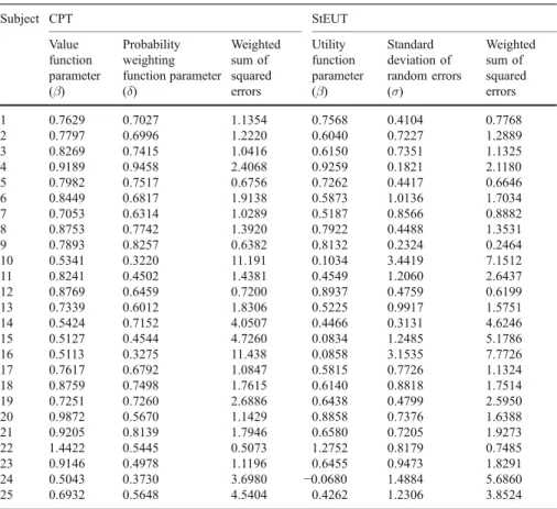
presents the results for lotteries with positive outcomes and Table2 does the same for lotteries with negative outcomes. For 19 out of 25 subjects, the utility function of StEUT has the same shape as the value function of prospect theory: concave for positive outcomes i.e. α∈(0,1) and convex for negative outcomes i.e. β∈(0,1). Standard deviation of random errorsσ varies from 0.0125, which indicates that an individual behaves according to EUT, to 3.4419, which indicates that an individual assigns certainty equivalents essentially at random. For 16 out of 25 subjects, standard deviation of random errors σ is lower when lotteries have negative outcomes than when lotteries have positive outcomes. One interpretation of this finding might be that the subjects are more diligent (less vulnerable to error) when making decisions involving losses.

The prediction of StEUT and CPT are very similar (correlation coefficient is 0.95 for lotteries with positive outcomes and 0.93 for lotteries with negative outcomes). Nevertheless, Table 1 shows that StEUT fits better than CPT for 15 out of 25 subjects, in the dataset where lotteries involve gains. Similarly, Table2 shows that StEUT achieves a lower weighted sum of squared errors for 14 out of 25 subjects, in the dataset where lotteries involve losses.

Gonzalez and Wu (1999) conducted a similar experiment to Tversky and Kahneman (1992). They recruited ten subjects to elicit their certainty equivalents of 165 lotteries with positive outcomes. For this dataset, the prediction of StEUT is estimated along the procedure already outlined above. Gonzalez and Wu (1999) estimated CPT with a probability weighting function wþð Þ ¼p δpγ=ðδpγþ

1p

ð ÞγÞand I use this functional form as well to estimate the prediction of CPT. For every subject, three coefficients of CPT (power coefficient α of the value function, curvature coefficient γ and elevation coefficient δ of the probability weighting function) are estimated to minimize the corresponding weighted sum of squared errors. The results of parametric fitting for StEUT and CPT are presented in Table3. StEUT fits better than CPT for all ten subjects in the sample. A possible explanation for such superior explanatory power of StEUT is that the dataset is quite noisy. Gonzalez and Wu (1999) report themselves that weak monotonicity is violated in 21% of the pairwise comparisons of the elicited certainty equivalents. Therefore, it is not really surprising that the model with an explicit noise structure fits the data very well.

6_{Specifically, the utility of lotteryL(x1,p1;...xn,pn) with outcomesx}

1<. . .<xm<0xmþ1<. . .<xn is eu Lð Þ ¼Pm_i¼1uð Þxi wPi_j¼1pjwPi_j1_¼1pjþPn_i¼mþ1uþð ÞxiwþP_jn_¼ipjwþPn_j¼iþ1pj,

w h e r e uð Þ ¼ x λðxÞβ, uþð Þ ¼x xα, wþð Þ ¼p pγ=ðpγ þð1pÞγÞ1=γ a n d wð Þ ¼p pδ

pδþð1pÞδ 1=δ _.

Table 2 Tversky and Kahneman (1992) dataset (lotteries with negative outcomes) Subject CPT StEUT Value function parameter (β) Probability weighting function parameter (δ) Weighted sum of squared errors Utility function parameter (β) Standard deviation of random errors (σ) Weighted sum of squared errors 1 0.7629 0.7027 1.1354 0.7568 0.4104 0.7768 2 0.7797 0.6996 1.2220 0.6040 0.7227 1.2889 3 0.8269 0.7415 1.0416 0.6150 0.7351 1.1325 4 0.9189 0.9458 2.4068 0.9259 0.1821 2.1180 5 0.7982 0.7517 0.6756 0.7262 0.4417 0.6646 6 0.8449 0.6817 1.9138 0.5873 1.0136 1.7034 7 0.7053 0.6314 1.0289 0.5187 0.8566 0.8882 8 0.8753 0.7742 1.3920 0.7922 0.4488 1.3531 9 0.7893 0.8257 0.6382 0.8132 0.2324 0.2464 10 0.5341 0.3220 11.191 0.1034 3.4419 7.1512 11 0.8241 0.4502 1.4381 0.4549 1.2060 2.6437 12 0.8769 0.6459 0.7200 0.8937 0.4759 0.6199 13 0.7339 0.6012 1.8306 0.5225 0.9917 1.5751 14 0.5424 0.7152 4.0507 0.4466 0.3131 4.6246 15 0.5127 0.4544 4.7260 0.0834 1.2485 5.1786 16 0.5113 0.3275 11.438 0.0858 3.1535 7.7726 17 0.7617 0.6792 1.0847 0.5815 0.7726 1.1324 18 0.8759 0.7498 1.7615 0.6140 0.8818 1.7514 19 0.7251 0.7260 2.6886 0.6438 0.4799 2.5950 20 0.9872 0.5670 1.1429 0.8858 0.7376 1.6388 21 0.9205 0.8139 1.7946 0.6580 0.7205 1.9273 22 1.4422 0.5445 0.5073 1.2752 0.8179 0.7485 23 0.9146 0.4978 1.1196 0.6455 0.9473 1.8291 24 0.5043 0.3730 3.6980 −0.0680 1.4884 5.6860 25 0.6932 0.5648 4.5404 0.4262 1.2306 3.8524

Table 3 Gonzalez and Wu (1999) dataset

Subject CPT StEUT Value function parameter (α) Curvature of probability weighting function (γ) Elevation of probability weighting function (δ) Weighted sum of squared errors Utility function parameter (α) Standard deviation of random errors (σ) Weighted sum of squared errors 1 0.5426 0.2253 0.3799 44.774 0.0955 2.1386 37.392 2 0.4148 0.3314 1.0153 27.241 0.3305 1.5108 19.162 3 0.5575 0.2665 1.4461 10.145 0.7155 1.7907 10.126 4 0.6321 0.2058 0.1523 40.382 −0.056 3.3712 26.255 5 0.3853 0.2351 0.915 17.368 0.2052 2.0611 13.435 6 1.3335 1.1966 0.4634 14.621 0.7546 0.3539 12.229 7 0.5306 0.2349 0.4106 25.176 0.1123 3.382 17.076 8 0.5184 0.4773 0.1263 61.97 –0.171 1.4185 37.992 9 1.1011 0.9363 0.2209 15.747 0.3776 0.6134 10.165 10 0.5991 0.5634 0.4315 36.291 0.2197 0.8115 28.311

3.3 Experiments with repeated choice

This section reexamines the experimental data from Hey and Orme (1994) and Loomes and Sugden (1998). In both studies the subjects faced a binary choice under risk and every decision problem was repeated again after a short period of time. Hey and Orme (1994) recruited 80 subjects to make 2×100 choice decisions between two lotteries with a possibility of declaring indifference. Hey and Orme (1994) constructed the lotteries using only four outcomes: £0, £10, £20 and £30. This convenient feature of the dataset allows us to estimate the utility function of StEUT without committing to a specific functional form (9). Since von Neumann-Morgenstern utility function can be arbitrarily normalized for two outcomes, we can fixuð Þ ¼U0 0 anduðU10Þ ¼1. The remaining parametersu1 ¼uðU20Þandu2¼

uðU30Þ capture the curvature of utility function and they are estimated from the observed choices.

The probability that lotterySwith the lowest outcomexS

1 and the highest outcome

xS

n is preferred to lotteryRwith the lowest outcomexR1 xS1 and the highest outcome

xR n xSn is equal to probðS RÞ ¼ R u xSð Þ_nμS u xS 1 ð ÞμS 6RðvþμSμRÞd6Sð Þv 6Sðu xð ÞSn μSÞ6Sðu xð ÞS₁ μSÞ 6R u xR 1 μR 6R u xR n μR 6R u xR 1 μR : ð11Þ

Explicit derivation of Eq.11can be found in the working paper Blavatskyy (2005). For every subject, three parameters of StEUT (σ, u1 and u2) are estimated to maximize log-likelihood

X

S

X

R alogprob Sð RÞ þblog 1ð prob Sð RÞÞ þc

logprob Sð RÞ þlog 1ð prob Sð RÞÞ

2

;

ð12Þ whereais the number of times the subject has chosen lotterySover lotteryR,b is the number of times the subject preferredR toS and cis the number of times the subject declared that he or she does not care which lottery to choose.

An individual who expresses indifference is assumed to be equally likely to choose either lotteryS or lotteryR(i.e. each lottery is chosen with probability one-half). This interpretation of indifference is motivated by popular experimental procedures. For subjects who reveal indifference, a choice decision is typically delegated to an arbitrary third party (e.g. a coin toss or a random number generator). Thus, if individuals reveal no preference for either lottery S or lottery R, they typically end up facing a 50–50% chance of playing either lottery S or lottery R, which is equivalent to the situation when they deliberately choose each lottery with probability one-half. Alternatively, indifference in revealed choice can be treated as an event when the difference in stochastic utilities of two lotteries does not exceed the threshold of a just perceivable difference as modeled in Hey and Orme (1994). The utility of a lottery according to CPT is calculated using the probability weighting function wþð Þ ¼p pγ

.

pγþð1pÞγ

ð Þ1=γ _{and the value function u}þ_{ð Þ ¼U0 0,}

it has to be embedded into a stochastic choice model to yield a probabilistic prediction. Like Hey and Orme (1994), I estimate CPT embedded in the Fechner model.7Specifically, the probability that lotterySis preferred to lotteryRaccording to CPT is

probðSRÞ ¼160;ρðeu Rð Þ eu Sð ÞÞ; ð13Þ whereΦ0,p(.) is the cumulative distribution function of the normal distribution with zero mean and standard deviationρ, andeuð Þ: is the utility of a lottery according to CPT. For every subject, four parameters of CPT (u1, u2,γ and ρ) are estimated to maximize the corresponding log-likelihood (12).

For all 80 subjects, the estimated best fitting parameters of StEUT satisfy weak monotonicity, i.e.u2≥u1≥1. However, for 14 subjects the estimated parameters are

u2=u1=1, which suggest that these subjects simply maximize the probability of

“winning at least something.” For 19 subjects the estimated parameter γ of a probability weighting function of CPT is greater than one, which contradicts the psychological foundations of CPT (Tversky and Kahneman1992). Additionally, for one subject the estimated value function of CPT violates weak monotonicity. For these 20 subjects, whose unconstrained best fitting parameters of CPT are

0 2 4 6 8 10 12 14 16 18 20 z>3.090 Vuong's adjusted likelihood ratio statistic Number of subjects

Akaike Information Criterion Schwarz Criterion

Predictions of StEUT and CPT are not significantly different Prediction of CPT is significantly better at

p≤0.1% p 1% p 5% p 10%≤ ≤ ≤

Prediction of StEUT is significantly better at p 10% p 5% p 1% p 0.1% z≤-3.090 -3.090< z≤-2.326 -2.326< z≤-1.645 -1.645< z≤-1.282 -1.282< z≤-0.675 -0.675< z≤0 0<z≤ 0.675 0.675< z≤1.282 1.282< z≤1.645 1.645< z≤2.326 2.326< z≤3.090 ≤ ≤ ≤ ≤

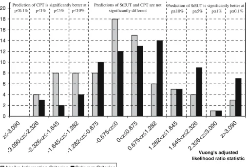
Fig. 1 Hey and Orme (1994) dataset (N=80)

7_{I also estimated CPT with a stochastic choice model probðSRÞ ¼1=ð1þexpfτðeu Rð Þ u Seð ÞÞgÞ,τ=} const, proposed by Luce and Suppes (1965, p.335) and used by Camerer and Ho (1994) and Wu and Gonzalez (1996). The result of this estimation was nearly identical to the estimation of CPT with the Fechner model.

inconsistent with the theory, the parameters of CPT are estimated subject to the constraintsγ≤1 andu2≥u1≥1.

StEUT and CPT are non-nested models that can be compared through Vuong’s adjusted likelihood ratio test (Vuong1989). Loomes et al. (2002, p.128) describe the application of Vuong’s likelihood ratio test to the selection between stochastic decision theories. Vuong’s statistic z has a limiting standard normal distribution if StEUT and CPT make equally good predictions. A significant positive value of z

indicates that StEUT fits the data better and a significant negative value indicates that CPT makes more accurate predictions. Figure 1 demonstrates that for the majority of subjects the predictions of StEUT and CPT (embedded into the Fechner model) are equally good. The number of subjects for whom the prediction of CPT is significantly better (worse) than the prediction of StEUT appears to be higher if we use Akaike (Schwarz) information criterion to adjust for the lower number of parameters in StEUT.

Loomes and Sugden (1998) recruited 92 subjects and asked them to make 2×45 binary choice decisions designed to test the common consequence effect, the common ratio effect and the dominance relation. The subjects faced a choice between lotteries with only three possible outcomes. For 46 subjects these outcomes were £0, £10 and £20, and for the other 46 subjects—£0, £10, and £30. Therefore, the utility function of StEUT is normalized so thatuð Þ ¼U0 0, uðU10Þ ¼1 and the remaining utilityu1¼uðU20Þor u1¼uðU30Þ(as appropriate) is estimated from the observed choice decisions. The same normalization is used for the value function of CPT. For every subject, two parameters of StEUT (σandu1) and three parameters of

0 2 4 6 8 10 12 14 16 18 20 22 Vuong's adjusted likelihood ratio statistic Number of subjects

Akaike Information Criterion Schwarz Criterion Prediction of CPT is significantly better at

p 0.1% p 1% p 5% p 10%

Predictions of StEUT and CPT are not significantly different

Prediction of StEUT is significantly better at p 10% p 5% p 1% p 0.1% z>3.090 z≤-3.090 -3.090< z≤-2.326 -2.326< z≤-1.645 -1.645< z≤-1.282 -1.282< z≤-0.675 -0.675< z≤0 0<z≤ 0.675 0.675< z≤1.282 1.282< z≤1.645 1.645< z≤2.326 2.326< z≤3.090 ≤ ≤ ≤ ≤ ≤ ≤ ≤ ≤

CPT embedded in the Fechner model (u1,γandρ) are estimated to maximize the log-likelihood (12) as already described above.

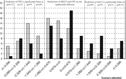
Estimated best fitting parameteru1of StEUT satisfies strong monotonicity, i.e.u1> 1, for all 92 subjects. However, 38 subjects have an S-shaped probability weighting function of CPT, i.e. the estimated best fitting parameterγis greater than one, which is at odds with the psychological foundations of the prospect theory. Among these 38 subjects, four individuals also have a non-monotone value function, i.e.u1<1. For these 38 subjects, the best fitting parameters of CPT are estimated subject to the constraintsγ≤1 andu1≥1. The predictive power of StEUT and CPT (embedded in the Fechner model) is compared based on Vuong’s adjusted likelihood ratio test. Figure2demonstrates that for the majority of subjects the predictions of StEUT and CPT are not significant different from each other. Thus, StEUT fits the experimental data in Loomes and Sugden (1998) and Hey and Orme (1994) at least as well as CPT. 3.4 Other experiments

This section reexamines the experimental results reported in Conlisk (1989), Kagel et al. (1990), Camerer (1989,1992), Camerer and Ho (1994) and Wu and Gonzalez (1996). In these experimental studies subjects were asked to make a non-repeated choice between two lotteries without the possibility to declare indifference.8 For every binary choice problem, the prediction of StEUT is calculated through Eq.11

using functional forms (8)–(9) and the prediction of CPT—through Eq.13using the functional form proposed by Tversky and Kahneman (1992) (see footnote 6). For every experimental dataset, two parameters of StEUT (eitherαorβ, andσ) and three parameters of CPT embedded into the Fechner model (eitherα,γandρorβ,δand

ρ) are estimated to maximize the corresponding log-likelihood (12), wherea now denotes the number of individuals who have chosen lotterySover Rand bdenotes the number of individuals who preferred R to S. Since there is no possibility of declaring indifference,cis set to zero for every dataset. Of course, individuals do not share identical preferences. However, a single-agent stochastic model is a simple method for integrating data from many studies, where individual estimates have low power, e.g. when one subject makes only a few decisions (Camerer and Ho1994, p.186). Such an approach is also relevant in an economic sense because it describes the behavior of a“representative agent”(Wu and Gonzalez1996).9

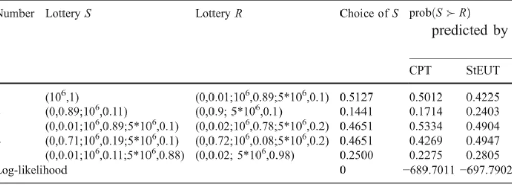
Table4presents five binary choice problems from Conlisk (1989). Conlisk (1989) replicates the Allais paradox in Problems no. 1 and 2. Problems no. 3 and 4 constitute a common consequence problem without a degenerate lottery that delivers one million for certain. Table 4 shows that the incidence of the Allais paradox

8_{Kagel et al. (1990) allowed the subjects to express indifference but do not report how many subjects} actually used this possibility. Camerer (1989) allowed indifference in one experimental session. Camerer (1989) reports that three subjects revealed indifference in almost every decision problem, and the rest never expressed indifference.

9_{There is also a practical constraint why the reexamination of individual choice patterns is not feasible.} Many of the experimental studies reexamined in this section were conducted over a decade ago and several authors, whom I contacted, could not find raw experimental data.

completely disappears in Problems no. 3 and 4. Finally, Problems no. 1 and 5 constitute a variant of the Allais paradox, when a probability mass is shifted from the medium to the highest (not lowest) outcome. Table 4 shows that the switch in preferences between lotteriesSandRacross Problems no. 1 and 5 is comparable to that in Problems no. 1 and 2 (the original Allais paradox).

Maximum likelihood estimates of the parameters of StEUT areα=0.6711 andσ= 0.8764. The best fitting parameters of CPT are α=0.4882, γ=0.4713 and ρ= 208.0832. CPT predicts very well the original Allais paradox; however, it also predicts the common consequence effect for Problems no. 3 and 4, which is not found in the data. StEUT makes a less accurate prediction for the original Allais paradox but it predicts no common consequence effect for Problems no. 3 and 4. Vuong’s likelihood ratio statistic adjusted through Schwarz criterion isz=−1.0997,

which suggests that the predictions of CPT and StEUT are not significantly different from each other according to conventional criteria.

Table5presents experimental results for human subjects from Kagel et al. (1990). The upper number in every cell shows the number of subjects who revealed each of four choice patterns that are theoretically possible in the experiment. Kagel et al. (1990) found frequent violations of EUT that are consistent with both fanning-out (higher risk aversion for stochastically dominating lotteries) and fanning-in (higher risk seeking for stochastically dominating lotteries) of indifference curves.

The second number in the second row of every cell shows the prediction of StEUT. Maximum likelihood estimates of StEUT parameters areα=0.7112, andσ= 0.2549. StEUT predicts fanning-out in the first set of lotteries, and fanning-in—in the second set of lotteries and non-systematic violations of EUT—in the third set of lotteries. In contrast, CPT explains these choice patterns only when its probability weighting function has an atypical S-shaped form (estimated parameterγ>1). The first number in the second row of every cell in Table 5 shows the prediction of unrestricted CPT. When the parameters of CPT are restricted, i.e.γ≤1, its fit (log likelihood−125.839) is worse than the fit of StEUT (log likelihood−125.095) even though CPT embedded in the Fechner model has more parameters.

Table6presents the results of estimation of CPT and StEUT on the experimental data reported in Camerer (1989,1992). In both studies, binary choice problems are

Table 4 Conlisk (1989) dataset: the fraction of subjects choosingSoverRin the experiment and the

prediction of CPT (α=0.4628,γ=0.4553,ρ=133.381) and StEUT (α=0.5314,σ=1.8367)

Number LotteryS LotteryR Choice ofS probðSRÞ

predicted by CPT StEUT 1 (106,1) (0,0.01;106,0.89;5*106,0.1) 0.5127 0.5012 0.4225 2 (0,0.89;106_{,0.11) (0,0.9; 5*10}6_{,0.1) 0.1441 0.1714 0.2403} 3 (0,0.01;106_,0.89;5*106_{,0.1) (0,0.02;10}6_,0.78;5*106_{,0.2) 0.4651 0.5334 0.4904} 4 (0,0.71;106,0.19;5*106,0.1) (0,0.72;106,0.08;5*106,0.2) 0.4651 0.4269 0.4947 5 (0,0.01;106,0.11;5*106,0.88) (0,0.02; 5*106,0.98) 0.2500 0.2275 0.2805 Log-likelihood 0 −689.7011−697.7902

constructed to test the betweenness axiom, the common consequence effect and the fourfold pattern of risk attitudes. The important feature of the experimental design in Camerer (1992) is that all lotteries have the same range of possible outcomes (lotteries are located inside the probability triangle e.g. Machina 1982). Camerer (1992) finds no significant evidence of the common consequence effect. This result is apparent in Table6. For the Camerer (1992) dataset, the best fitting parameterσof StEUT is close to zero, which is a special case when StEUT coincides with EUT. When lotteries involve small outcomes, the parameter of probability weighting function of CPT is close to one, which is a special case when CPT coincides with EUT.

We compare the fit of CPT and StEUT, as before, using Vuong’s adjusted likelihood ratio statistic z (significant positive values indicate that StEUT better explains the observed choice patterns). Table6shows that CPT explains significantly better than StEUT the choices over lotteries with large positive outcomes from Camerer (1989). StEUT explains significantly better than CPT the choices over lotteries with small positive and negative outcomes from Camerer (1992). For the remaining experimental data, the predictions of CPT and StEUT are not significantly different. Interestingly, for experimental data from Camerer (1989), parameterσ of StEUT is lower when real rather than hypothetical incentives are used, suggesting that monetary incentives reduce random variation in the experiments (Hertwig and Ortmann2001). It is also lower when lotteries involve negative outcomes suggesting that subjects are more diligent when faced with the possibility of losses. These observations support the interpretation of parameterσ as the standard deviation of random errors, which are specific to the experimental treatment.

Camerer and Ho (1994) designed an experiment to test for the violations of the betweenness axiom. Table 7 presents the frequency with which all theoretically possible choice patterns are actually observed in their experiment, as well as the predicted frequencies according to CPT (embedded into the Fechner model) and StEUT. The predictions of CPT and StEUT are correspondingly the first and the second

Table 5 Kagel et al. (1990) dataset: the upper number in every cell is the number of subjects who

revealed a corresponding choice pattern in the experiment; the lower numbers in every cell are the predicted numbers of subjects according to CPT (first number) with best fitting parametersα=0.4,γ= 2.0127,ρ=1.6165 and StEUT (second number) with parametersα=0.7112,σ=0.2549

T able 6 Ca merer ( 1989 , 1992 ) dataset Ex periment Incentives Cumula tive pros pect theory (embedded into Fe chner mode l) Stocha stic expec ted utility theo ry V uong ’ s adju sted likelihood ratio V alue function parameter (α or β ) Proba bility weigh ting function parameter (γ or δ ) Standard deviation of random errors ( ρ ) Log likelihood Utility function parameter (α

or β ) Standa rd deviation of ran dom errors (σ ) Log likelihood Akaik e Inf ormation criterion Schw arz criterion Ca merer ( 1989 ), lar ge positiv e outcome s Hypoth etical 0.43 16 0.71 01 13.7896 − 883. 842 0.29 49 0.50 65 − 895. 551 − 2.62 9 b − 1.98 6 a Ca merer ( 1989 ), sma ll positiv e outcome s Rando m lottery ince ntive scheme 0.98 81 0.99 75 0.0516 − 945. 091 0.51 90 0.33 83 − 947. 523 − 0.49 85 +0.41 55 Ca merer ( 1989 ), sma ll neg ative outcome s Rando m lottery ince ntive scheme 0.00 00 0.82 85 0.4141 − 908. 124 0.87 72 0.04 33 − 91 1.541 − 1.19 49 +0.10 41 Ca merer ( 1992 ), lar ge positiv e outcome s Hypoth etical 0.01 41 0.61 77 0.3508 − 502. 552 0.58 5 0.08 68 − 505. 623 − 0.72 38 +0.20 34 Ca merer ( 1992 ), sma ll positiv e outcome s Hypoth etical 0.98 47 0.99 81 0.1063 − 490. 652 0.87 29 0.09 14 − 490. 618 +3.24 8 c +10.4 7 c Ca merer ( 1992 ), sma ll neg ative outcome s Hypoth etical 0.95 20 0.99 12 0.1236 − 521. 269 0.69 51 0.09 17 − 522. 543 +4.40 7 c +6.54 4 c aSignific ant at 5% (one-sided test) b Sign ificant at 1% (one-sided test) c Signific ant at 0.1% (one -sided test)

number in the second line of every cell. Estimated CPT parameters areα=0.5555,γ= 0.9324, andρ=1.0689, and estimated StEUT parameters areα=0.4812 andσ=0.1178. Table 7 shows that the predictions of CPT and StEUT are remarkably similar. Vuong’s adjusted likelihood ratio statistic is z=−0.4521 based on Akaike Information Criterion and z=+0.636 based on Schwarz Criterion. Although both theories fit the experimental data in Camerer and Ho (1994) quite well, they fail to explain a modal quasi-concave preference in the last lottery triple, which is a replication of a hypothetical choice problem originally reported in Prelec (1990). Apparently, the parameterizations of StEUT (and CPT) compatible with an asymmetric split between quasi-concave and quasi-convex preferences, when a modal choice pattern is consistent with the betweenness axiom, cannot explain such an asymmetric split when a modal choice pattern violates betweenness.

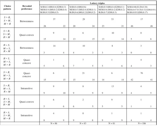
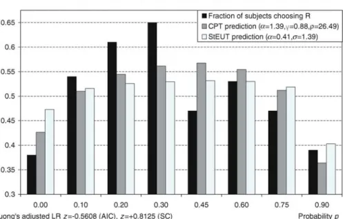
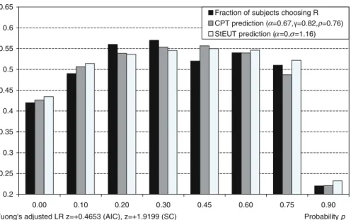
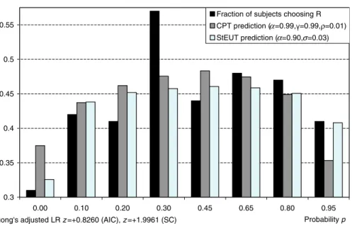
Wu and Gonzalez (1996) study the common consequence effect using 40 binary choice problems grouped into five blocks (“ladders”). Eight problems grouped within one block can be derived from each other by shifting the same probability mass from the lowest to the medium outcome. Wu and Gonzalez (1996) find that the fraction of subjects choosing a more risky lotteryRfirst increases and then decreases when the probability mass is shifted from the lowest to the medium outcome (Figures3,4and 5).

Table 7 Camerer and Ho (1994) dataset: the upper number in every cell is the number of subjects who

revealed a corresponding choice pattern in the experiment; the lower numbers in every cell are the predicted numbers of subjects according to CPT (first number) with best fitting parametersα=0.5555,γ= 0.9324,ρ=1.0689 and StEUT (second number) with parametersα=0.4812,σ=0.1178

Lottery triples S($0,0.3;$80,0.4;$200,0.3) M($0,0.4;$80,0.2;$200,0.4) R($0,0.5;$200,0.5) S($0,0.4;$80,0.6) M($0,0.5;$80,0.4;$200,0.1) R($0,0.6;$80,0.2;$200,0.2) S($0,0.5;$80,0.4;$200,0.1) M($0,0.6;$80,0.2;$200,0.2) R($0,0.7;$200,0.3) S($0,0.66;$120,0.34) M($0,0.67;$120,0.32;$200,0.01) R($0,0.83;$200,0.17) 37 29 33 17 26 22 20 24 23 21 46 46 15 14 13 15 13 14 5 6 14 10 8 3 3 4 4 3 3 3 0 0 1 7 1 4 5 6 7 5 5 6 4 3 6 21 6 76 15 15 15 14 14 14 42 41 9 8 13 4 9 10 9 9 9 9 4 5 6 2 9 1 5 6 6 5 5 5 1 1 4 0 1 1 8 9 9 8 9 9 4 4 Choice pattern Revealed preference , R S , M S R M Betweenness , R S , M S M R Quasi-convex , S R , S M M R Betweenness , S R , S M R M Quasi-concave , R S , S M R M Quasi-concave , R S , S M M R Intransitive , S R , M S M R Quasi-convex , S R , M S R M Intransitive N = 86 N = 83 N = 81 N = 106 9 6 10 0

Figures3,4and5demonstrate the predictions of CPT (embedded in the Fechner model) and StEUT about the fraction of subjects who choose a more risky lotteryR. The predictions of CPT and StEUT replicate the generalized common consequence effect, though the predicted effect appears to be not as strong as in the actual experimental data. According to Vuong’s likelihood ratio test adjusted though Akaike Information Criterion, the predictions of CPT and StEUT are not significantly different from each other. Vuong’s likelihood ratio test adjusted though Schwarz Criterion shows that the prediction of StEUT is closer to actual choice data than the prediction of CPT in ladders 2 and 5.

4 Conclusion

New decision theory—stochastic expected utility theory (StEUT)—is proposed to describe individual decision making under risk. Existing experimental evidence demonstrates that individuals often make inconsistent decisions when they face the same binary choice problem several times. This empirical evidence can be interpreted that individual preferences over lotteries are stochastic and represented by a random utility model e.g. Loomes and Sugden (1995). Alternatively, an observed randomness in revealed choice under risk can be due to errors that occur when individuals execute their deterministic preferences. This paper follows the latter approach. Individual preferences are fully captured by a non-decreasing Bernoulli utility function defined over changes in wealth rather than absolute wealth levels. However, individuals make random errors when calculating the expected utility of a risky lottery.

Simple models of random errors have already been proposed in the literature when the probability of an error (Harless and Camerer1994) or the distribution or errors (Hey and Orme1994) was assumed to be constant for every choice problem. Such assumptions are clearly too simplistic because individuals obviously make no errors when choosing between “sure things” (degenerate lotteries) and very few errors—when one of the lotteries (transparently) first-order stochastically dominates the other lottery (Loomes and Sugden1998). On the other hand, when individuals choose between more complicated lotteries they switch their revealed preferences in nearly one third of all cases (Camerer1989).

StEUT assumes that although individuals make random errors when calculating the expected utility of a lottery, they do not make transparent errors and always evaluate the lottery as at least as good as its lowest possible outcome and at most as good as its highest possible outcome. In other words, the internality axiom is imposed on the stochastic expected utility of a lottery, which is defined as expected utility of the lottery plus an error additive on the utility scale. Apart from this restriction, the distribution of random errors is assumed to be symmetric around zero.

These intuitive assumptions about the distribution of random errors immediately imply that the lotteries whose expected utility is close to the utility of its lowest (highest) possible outcome are likely to be overvalued (undervalued) by random errors. Therefore, on the one hand, random errors reinforce risk-seeking behavior when the utility of a lottery is close to the utility of its lowest outcomes (e.g. unlikely gains or probable losses). On the other hand, random errors reinforce risk averse

behavior when the utility of a lottery is close to the utility of its highest outcomes (e.g. probable gains or unlikely losses). Thus, StEUT can explain the fourfold pattern of risk attitudes. The paper also shows that StEUT is consistent with the common consequence effect, the common ratio effect, and the violations of betweenness.

To assess the descriptive merits of StEUT, the experimental data from ten well-known empirical studies are reexamined. Ten selected studies are Conlisk (1989),

Kagel et al. (1990), Camerer (1989,1992), Tversky and Kahneman (1992), Camerer and Ho (1994), Hey and Orme (1994), Wu and Gonzalez (1996), Loomes and Sugden (1998) and Gonzalez and Wu (1999). Within-subject analysis shows that for the majority of individual choice patterns there is no significant difference between the predictions of StEUT and CPT. Between-subject analysis shows that StEUT

Choice of lottery R($0,0.97-p;$200,p;$320,0.03) over lottery S($0,0.95-p;$200,p+0.05)

0.25 0.3 0.35 0.4 0.45 0.5 0.55 0.6 0.00 0.10 0.20 0.30 0.45 0.65 0.85 0.95 Probability p

Fraction of subjects choosing R CPT prediction ( =0.71, =0.83, =1.7) StEUT prediction ( =0.17, =0.96)

Vuong's adjusted LR z=+0.1327 (AIC), z=+1.5773 (SC)

α σ

α ρ

Choice of lottery R($0,0.95-p;$50,p;$100,0.05) over lottery S($0,0.9-p;$50,p+0.1)

0.2 0.25 0.3 0.35 0.4 0.45 0.5 0.55 0.6 0.65 0.00 0.10 0.20 0.30 0.45 0.60 0.75 0.90 Probability p

Fraction of subjects choosing R CPT prediction ( =0.67, =0.82, =0.76) StEUT prediction ( =0, =1.16)

Vuong's adjusted LR z=+0.4653 (AIC), z=+1.9199 (SC)

α

α σ

ρ

explains the aggregate choice patterns at least as well as does CPT (except for the experiment with large hypothetical gains reported in Camerer 1989). Thus, a descriptive decision theory can be constructed by modeling the structure of an error term rather than by developing deterministic non-expected utility theories. For the brevity of exposition, StEUT is contested only against CPT (or rank-dependent expected utility theory), similar as in Loomes et al. (2002). A natural extension of this work is to evaluate the goodness of fit of several decision theories as it is done, for example, in Carbone and Hey (2000) and to compare their performance with the fit of StEUT.

StEUT does not satisfactorily explain all available experimental evidence such as the violation of betweenness when a modal choice pattern is inconsistent with the betweenness axiom (see the last column of Table7). Interestingly, CPT does not explain this phenomenon either, though it is able to predict such violations theoretically (Camerer and Ho1994). StEUT and CPT embedded into the Fechner model also predict too many violations of transparent stochastic dominance than are actually observed in the experiment. Loomes and Sugden (1998) argue that any stochastic utility model with an error term additive on the utility scale predicts, in general, too many violations of dominance. Thus, a natural extension of the present model is to incorporate a mechanism that reduces error in case of a transparent first-order stochastic dominance. Blavatskyy (2006b) develops such a model by reducing the standard deviation of random errors in decision problems where one choice option transparently dominates the other alternative.

To summarize, there is a potential for constructing an even better descriptive model than StEUT (and CPT) that explains the above mentioned choice patterns. The contribution of this paper is to demonstrate that this hunt for a descriptive

Choice of lottery R($0,0.97-p;$200,p;$320,0.03) over lottery S($0,0.95-p;$200,p+0.05)

0.3 0.35 0.4 0.45 0.5 0.55 0.00 0.10 0.20 0.30 0.45 0.65 0.80 0.95 Probability p Fraction of subjects choosing R CPT prediction ( =0.99, =0.99, =0.01) StEUT prediction ( =0.90, =0.03)

Vuong's adjusted LR z=+0.8260 (AIC), z=+1.9961 (SC)

α

α σ

ρ