An Efficient Priority Based Routing Technique That Maximizes the Lifetime and Coverage of Wireless Sensor Networks

(1)

An Efficient Priority Based Routing Technique That

Maximizes the Lifetime and Coverage of

Wireless Sensor Networks

Imad Salah1, Mohmmad A. Alshriedeh1, Saleh Al-Sharaeh2 1_{Department of Computer Science, The University of Jordan, Amman, Jordan}

2_{Department of Computer Science, Fahd Bin Sultan University, Tabuk, KSA} Email: [email protected], [email protected], [email protected]

Received November 26, 2012; revised December 15, 2012; accepted January 4, 2013

ABSTRACT

Recent development in sensor technologies makes wireless sensor networks (WSN) very popular in the last few years. A limitation of most popular sensors is that sensor nodes have a limited battery capacity that leads to lower the lifetime of WSN. For that, it raises the need to develop energy efficient solutions to keep WSN functioning for the longest period of time. Due to the fact that most of the nodes energy is spent on data transmission, many routing techniques in the literature have been proposed to expand the network lifetime such as the Online Maximum Lifetime heuristics (OML) and capacity maximization (CMAX). In this paper, we introduce an efficient priority based routing power management heuristic in order to increase both coverage and extend lifetime by managing the power at the sensor level. We accom- plished that by setting priority metric in addition to dividing the node energy into two ratios; one for the sensor node originated data and the other part is for data relays from other sensors. This heuristic, which is called pERPMT (priority Efficient Routing Power Management Technique), has been applied to two well know routing techniques. Results from running extensive simulation runs revealed the superiority of the new methodology pERPMT over existing heuristics. The pEPRMT increases the lifetime up to 77% and 54% when compared to OML and CMAX respectively.

Keywords: Wireless Sensor Networks; Energy-Aware Routing; Sensors Deployment; Priority Based Technique

1. Introduction

Recent advances in Nano-electromechanical systems (NEMS) paved the way to new applications for Wireless sensor networks [1-3]. Sensor networks comprise a large number of small-size nodes with sensing, computation, and wireless communication capabilities. These nodes collabo- rate together by performing desired measurements, process measured data, and transmitting it to some special nodes, commonly referred to as sink node [2]. One limitation to sensor nodes is the limited battery capacity [2,3]. Usually, the sensor nodes are deployed in a hard to reach areas. For that, it has a limited lifetime. Many researches in the literature have the objective to maximize the lifetime of sensor nodes by developing new routing techniques [4]. Hence, it is vital to develop solutions that are energy efficient and maximizing the network lifetime [1,4].

Energy depletion is mainly due to data reception and transmission, where the later is large when compared to data reception [2]. There are many ways for data to be received (collected) or propagate to end (sink node) node. Either by, single-hop transmission [5,6], multi-hop trans-

mission, or cluster-based transmission [1]. Single-hop transmission is the simplest transmission method which tries to communicate directly with the sink node, but this consumes higher power rates. Multi-hop transmission delivers data by forwarding it to one of its adjacent nodes, which are closer to the sink node; the data propagate from the source node to the sink from one node to another until it reaches the sink node. A drawback of this methodology, nodes closer to the sink must forward data received from other nodes as well as transmitting their own data to the sink base station. For that, their batteries drain quickly more than others, and as results produce blind areas and cause network partitions. In cluster based transmission [5,6], nodes are grouped into clusters and one node which is the cluster head is responsible of sending other nodes data to the sink.

(2)

way that will save power as much as possible so that the lifetime of the network is maximized.

Prolonging the lifetime is the same as increasing the coverage of WSN. By prolonging the lifetime of sensor node, the vicinity of sensor node area is kept covered [2,3]. One of our purposes was to keep all or most of the network nodes active (alive) most of the network lifetime.

The reminder of the paper is organized as follows: Section 2 introduces the wireless sensor networks mathematical model. In Section 3, we provide simulation and modeling of pERPMT. Simulation data and discussion of pERPMT is introduced in Section 4. Section 5 is con- cluding the paper.

2. Literature Review

The main problem in most of energy-aware routing heuristics is that they find the lowest energy route and use it for every communication [2,7,8]. Using low energy path more frequently will leads to energy depletion of the nodes along that path especially the nodes closer to the sink. Once the sensor node dies it leads to network parti- tion that cause blind areas (areas that can not be sensed by any node). Some heuristics have been proposed to solve this problem by taking into account the residual energy at nodes and delay the depletion of nodes that are already low in energy [9,10]. In [11], the researchers proposed the MRPC (Maximum Residual Packet Capa- city) lifetime-maximization, which depends not only on the residual battery energy on a node, but also on the expected energy spent in forwarding a packet over a specific link. MRPC selects the path that has the largest packet capacity at the node which has the smallest residual packet transmission capacity. They also present CMRPC, a conditional variant of MRPC that switches from MRPC only when the packet forwarding capacity of nodes falls below a predetermined threshold. In [12], they proposed the CMAX (Capacity Maximization). The capacity is the number of messages routed over some time period, heuristic which provides a single path for each message (no multiple paths) chosen with respect to the link weights. The heuristic makes admission control. That is, it rejects some routes that are possible in order to increase lifetime. In [13,14], the authors introduced localized heuristics to maximize lifetime in which they define a new power cost metric based on both nodes life time and distance-based power metrics. They also show that the required transmission power can be reduced if additional nodes placed at desired locations between two nodes at distance D. Park and Sahni [15] proposed the OML (Online Maximum Lifetime) heuristic where two shortest path computations are done to route each message. In order to maximize lifetime, we need to delay as

much as possible the depletion of a sensor’s energy to a level below that needed to transmit to its closest neighbor. Al-Sharaeh, et al. [16], introduced a Multi-Dimensional Poisson Distribution Heuristic to better evaluate the routing heuristics; by taking into account earth’s terrain and the multi-dimensional concept and this is done by the method of placement of sensors and the probability of the connections between sensors nodes. The positions of the sensors (x and y-coordinates) are chosen either from a Uniform or Poisson distributions. A major effect on the performance of different routing heuristics was gained. In [17], they introduced a study of the deployment strategy effect on maximizing the lifetime of the wireless sensor networks; it shows that changing the statistical techniques of distribution—such as Poisson Distribution— that meet real environment requirements affect the performance of maximizing lifetime routing heuristics in many aspects, such as average lifetime and network capacity. In [9] the authors prolonged the life time by proposing new heuristic based-on dividing the energy of nodes into two parts. The heuristic named an Efficient Routing Protocol Management Technique (ERPMT). The Alpha part reserved to own data transmission, while the Beta part for other nodes data (i.e. to relay other nodes data). One draw back of their work is that, the nodes close to the sink nodes, say, one hop, deplete their energy very fast as compared to two hops.

In this work, we proposed a heuristic that delays the depletion of one-hop nodes by adding a priority metric. The priority number that we have is based on two factors. One is the number of hopes and the second is based on the energy level of the node. In order to have fair comparison, we perform a battery power management at the node level with and without priority based scheme, such that the total power of the sensor battery is divided into two parts; the first is dedicated for sending data ge- nerated by the sensor itself, while the other is for data relays from other sensors [9,10]. Our approach can be used along with any existing routing heuristics. For that, we compared pERPMT against two well known routing heuristics: OML, CMAX, and ERPMT.

3. WSN Mathematical Model

A wireless sensor network is represented by a directed graph G



V E,



, where V is the set of nodes, and E is the set of edges between these nodes, there will be a directed edge from node v to node u (i.e.

 

v u, E) if u and v in the range of each others. Such modeling can be used to represent Wireless Sensor Networks (WSN). for each

 

u v, E, in case of single hop transmission from sensor u to sensor v, the current energy in sensor u, ce(u)

is represented by Equation (1) [12]

 



,

e e

(3)

where ce(u) is the current energy

 

w u v

 

, 0 in sensor u, such as

e

c u and is the energy required

to make a single hop transmission from sensor u to sen-sor v, such that w u v

 

, 0. We also assume that the receiver of a message consumes no energy during mes-sage reception. Thus, the current energy in sensor (v) is not affected by the transmission from u to v. In our work the energy is divided into two ratios, one for data origi-nated from the node (α), the other is for relays from other sensors (β); if the data is originated from the node itself, it will use the energy from the first ratio otherwise it will use energy from the other ratio.

An adjacency matrix can be used to represent directed graphs of WSN [12-16]. The adjacency m

 

,

w u v

atrix of a finite directed graph G on n vertices (where nV ), is the n × n matrix such that, the non-diagonal entry a i j

 

, 1, represents the existence of an edge from sensor i to sen-sor j. While the diagonal entry a i i

 

, is assigned by zeros here because we assume that there is no internal loops in the WSN.

There exists a unique adjacency matrix for each graph. For example, Figure 1(a) shows a simple representation

for sensor network S. A directed graph is used, where the represented nodes are sensors, and the edges represent the existence of edges between the sensor nodes. Figure 1(b) shows the adjacency matrix of the sensor network S

modeled in Figure 1(a). It is obvious that Figure 1(b)

depicts a network that has been implemented using one dimension to represent sensors. Such representation for sensors has been used by Al-Sharaeh, et al. [16].

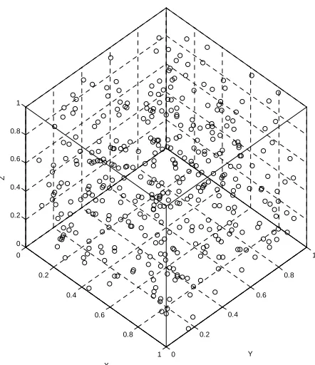
In most of the studies to represent a sensor location as well as connectivity a random number from Uniform distribution was used [12]. It is better to use the Uniform distribution for flat terrain environment, because the sensors can be distributed evenly as shown in Figure 2,

but the real environment usually characterized by terrains, such as in case of sensors deployed in high mountains or deep oceans. In this case, the Uniform distribution does not give a good realistic that match the terrain changes. For that, it is better to use Poisson distribution as it is best fits the asymmetric environment [16,17]. Figure 3

5

1

2

3

4

5

2 3 4 5

0 0 0 0 0

1 0 1 0 0

0 0 0 1 0

0 0 0 0 1

1 0 1 0 0 4

3

2

1

[image:3.595.314.535.82.338.2] [image:3.595.313.534.382.633.2] [image:3.595.60.286.591.699.2]

(a) (b)

Figure k, (a)

Simple nding

1. Representation of wireless sensor networ graph network representation; (b) Correspo adjacency matrix representation.

0

0.2

0.4

0.6

0.8

1 0 0.2

0.4 0.6

0.8 1 0

0.2 0.4 0.6 0.8 1

Y

X

Z

Figure 2. 3D Sensor nodes distribution based on Uniform distribution.

5

10

15

20

25

30

35

40 5 10

15 20

25 30

35 40 5

10 15 20 25 30 35

Y

X

Z

Figure 3. 3D Sensor nodes distribution based-on Poisson distribution.

nodes distribution based on Poisson distri-shows sensor

(4)

in the literature we used Uniform distribution.

An example of sensor deployment application is ava-lanching predictions, mountainous terrains portrait all the ch

ich was equal to the mean of the dimen-si

euristic

heuristics to apply pERPMT stics were proposed to

ex-r the C

[image:4.595.316.532.80.194.2] [image:4.595.58.285.572.711.2]

allenges that may face sensor deployment in order to make full coverage. For that, deployment strategy has a major effect on evaluating a routing heuristic. This is due to the fact of terrain changes of real life environment.

Figure 4 depicts the landscape of typical environment

that ranges from flat land, hilltop, cliffs, valleys, to mountains top. In order to make fair comparison between different routing protocols, a major attention should be paid to the deployment strategy. This factor can be taken into consideration by the way we generate the random graph that both simulate the position as well as the con-nectivity that at the end will simulate the way the sensors are connected.

To determine connectivity between the nodes, we used a threshold wh

ons of network nodes. All nodes were recursively checked by comparing their X-, Y- and Z-dimension in case of 3D deployment with the mean of the Euclidian dimensions for these 3 dimensions (X, Y, and Z) for all network nodes. For the case of 1D, we only work with just the X dimension. Each node with a dimension value greater than or equal to the mean of the same dimension will be considered connected, otherwise it will be dis-connected [16].

4. pERPMT H

We have used two well known on, these two different heuri

tend the lifetime of the network and they obtained the best lifetime in the literature, CMAX and OML.

Figure 5 shows the details of our proposed heuristic,

which is pERPMT_C and it is an enhancement ove MAX, where we assume that the current energy in each sensor is divided in two ratios, the first is for the sensor originated data (α), the other is for relays from other sensors (β). For each routing step there are three steps. In

a) Calculate the average power of each path

b) Assign a priorty number scalled to the corrosponding average power for _P_alli

I If _{P has a node in the range of the sink}_alli _,_{then the}

path of _{P with the maximum priority is selected}_alli _,

otherwise we use _P_alli

If no path is found in Step 3,the route is not possible

(network is considered dead (i.e. end of lifetime).

Figure 5. pERPMT based on CMAX heuristic.

ep o quate

1

st e

ne; every edge with a sensor that has not ade nergy to make a single hop transmission is eliminated from the graph. Then each remaining link is assigned a weight using Equation (2):

 

_,

 

_,



a u 



w u v w u v  c  (2)

where c

e of t

is a heuristic parameter,

centag e initial energy that ha

 

een spent

a u is the

per-h s already b

at the sensor node and calculated as in Equation (3):

 

   

1

1 c u i ue e

a u 

2

1 ce u i ue

 

 

  

Figure 4. Mountains terrains for avalanche detection WSN application.



 

 

In the second step, the source-to-d modi

th

(3)

estination path in the fied Graph is computed. If a path is not found, then e request failed. Otherwise it is used unless it is larger than a specified threshold σ. In the third step, we assign a priority number; it is range depends on the number of paths. The set value for the priority number depends on the average power of the path. Furthermore, since through extensive simulation runs we concluded that those nodes close to the sink depleted fast, for that we excluded those nodes from our computations. Since we excluded the nodes that are one hop far from the sink, only that path that has at least one node in the range of sink is selected. For the case if there is no node in the range of the sink, we include the one hope node in the calculated paths.

Assumption: Divide the current energy of each sensor

into ce1 andce2:

1 Total ergy

e

c  En  and ce₂Total Energyce₁

For each routing request r_i 



s t_i,_i



: Step 1: [Initialize]

Eliminate from G every edge



u v,



for which:

 

c ue1

 

w u



u si

r u 





 

2

, if , if

e

e i

v

c u w u v u s

 

 

  

 

 

 

 

u v,

Change the weight of every remaining edge to:

 

_,

 

_,



a u  ₁



c

w u v w u v   

c



n

(5)

sensor no e and it is calculated as:

 

d

   

1

1 c u i u_e a u    

2

1

e

e e

c u i u 



 

 

Step 2: [Shortest Paths]

Let be all shortest source-to-destination path in the modified Graph, and leall t

i P

alli

P be the average path power.

[image:5.595.306.536.91.463.2]

Step 3: [Path Selection that has highest priority] Figure 6 details of the second heuristic (ERPMT

ba on

C

s are ch that

sed on OML) are shown. As in ERPMT based MAX, we assume that the energy in each sensor is di-vided into two ratios α and β. Then for each routing re-quest ri 



s ti, i



,two steps are done:

Step 1: [Compute G′′] :

All edge removed from G su c ue1

 

ower th

g graph or

an

 

1 u w u v, ; as these e

c

requ



,



G V E . De

edges have less p

ired for a single transmission. The resultin is termine the minimum energy path pi

from s_i to t_i in G. This is done using a shortest m based on Dijikstra’s Algorithm. If ther is no th from the ource s to destination t, then the routing request fails, but if routing request exists, then

P is used to compute the residual energy using Equa-tion (4): path algorith pa e s

 





minREmin r u_e inP (4) Then the graph G



V E, 



can be

moving all edges

obtained by re-

 

u v, in E with

e graph and the reduction o

begin with

 

or 1

e

 

1 , m

e u w u v  result, all the edges with

residual energy be minRE) will be d fro f energy from sensors that are low on energy could be prevented.

The second step in the procedure is to find the path to be used to route the request r, we

c u

prune

inRE. As a low (

c

m th

G and as

ent epl

to its nearest neighbor in ) as expressed in Eq

sign weights to each

 

u v, in E; this is done to balance the desire to minimize total energy consumption as well as the desire to prev the d etion of a sensor’s energy.

Let eMin (the energy needed by sensor u to transmit a

message G

uation 5:

 



  



Min min , ,

e u  w u v u v E (5)

Now, let be defined as in the f tion: i     (6)

where the c symbol is a non-negative constant and it is an

 

u v, ollowing equa-

 

u v,



 

0,if , Min and

,Otherwise

e

e i

c u w u v e u u s

c            

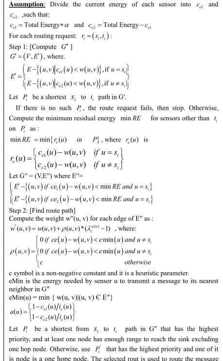
Assumption: Divide the current energy of each sensor into ce1 and 2

e

c ,such that:

1 Total Energy

e

c   and ce2Total Energyce1

For each routing request: ris ti,i:

Step 1: [Compute G]

 , 

GV E, where.

     





   



, e2( ) ,



,if i

E u v c u w u v u s 1

, e , ,if i

E u v c u w u v u s

E      

  

 

 

Let Pi be a shortest si to ti path in G′.

If there is no such Pi, the route request fails, then stop. Otherwise,

Compute the minimum residual energy minRE for sensors other than ti

on Pi as :

 

minRE min r ue( ) in P , where r ue( ) is

           i e i e

e _c _u _w_u_v _if_u _s

s u if v u w u c u r ) , ( ) ( ) , ( ) ( ) ( 2 1

Let G′′ = (V,E′′) where E′′=

                1 2

, , min

i i E u v if ce u w u v RE and u s E u v if ce u w u v RE and u s

     

 

    



Step 2: [Find route path]

Compute the weight w′′(u, v) for each edge of E′′ as :

''_{( , )} _{( , )} _{( , )*(} a u( ) ₁₎

c

w u v w u v u v   , where:

 

     

0 , min

, 0 , min

i i if ce u w u v e u and u s u v if ce u w u v e u and u s

c otherwise            

c symbol is a non-negative constant and it is a heuristic parameter. eMin is the energy needed by sensor u to transmit a message to its nearest neighbor in G″

eMin(u) = min { w(u, v)|(u, v) Є E″}

1 2

1 ( ) ( )

( )

1 ( ) ( )

e e

c u i u a u

c u i u



 

  _ 

 

Let Pi be a shortest from si to ti path in G″ that has the highest

priority, and at least one node has enough range to reach the sink excluding

one hop node.Otherwise, use ''

i

P that has the highest priority and one of it

is node is a one hope node. The selected rout is used to route the message from si to ti.

Figure 6. pERPMT based on OML heuristic.

algorithm parameter. Then a (u) is defined for each u in V as a

 

u minRE c ue1

 

or c ue1

 

and the weight

 

,

w u v

using Eq

assigned to edge puted

uation (7):

 

,

u v in E is com

 

,

 

,

 

,



a u 1



c

w u v w u v  u v     (7)

where _c is another non-negative constant an algorithm paramete

n be seen, the weight funct , through r.

As ca ing ion ,

assigns a high weight to edg ose on a routing path causes a sensor

es wh use

’s residual energy to become low. Also, all edges emanating from a sensor who

energy is small relative to minRE are assigned a high be

the use of edges whose use on a routing path

is ly

se current

weight cause of the term. Thus the weighting function discourages

(6)

5.

te

niform. In each of 10 net sors

ni ution.

gle-hop t on be-

Expremintals Results

The pERPMT is implemented using _MatLabTM_soft-

ware running on a Operating System of Windows XP SP3 installed on a PC with 3.20 GHz processor and 2 GB of RAM. The OML and the CMAX were implemented using the new power management chnique (pERPMT)

based on U works 20 sen

form distrib ransmissi

0.001 d were randomly populated based on U

The energy required by a sin

tween two sensors was assumed to be _ 3_{, and}

the Euclidean distance between two sensors is d. And the transmission radius and initial energy for each sensor were set to 5100 respectively. Finally, the c was set to

3

0.001rT , where rT is the transmission radius [12].

The simulation results show the effects of applying the power management technique in different distribution types on the network lifetime.

A. Dedicatingpowerlessthanorequal

Here α was 50%, 40%, 30%, 20%, and 10% f total node energy.

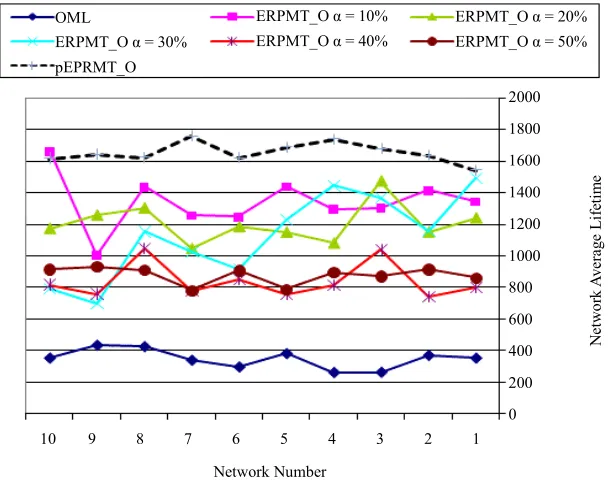
1) Averagelifetimefor

toβforα

o

 

ty sensor etworks were deployed to be ran-domly distributed. Figure 7 depicts the average lifetime

for 10 networks with 20 sensors in each network for the OML and pERPMT_O (pERP

A twen n

MT based on OML)

heu-ris PMT

technique t

bservation is found when as we use CMAX,

de previous researches in [16,17],

w

0%, 80%, 90%, 100%.

is clear that as the power

de rated data increases,

th

y, but as we discussed before that C

ult is ne

B. Dedicatingmorepowerforαthanβ

In these experiments α was larger than β, α was set to 60%, 7

1) Averagelifetimeforα>β

Figure 9 shows the results of applying the pERPMT

on the OML (pEPRMT_O). It dicated for the sensor own gene

e lifetime decreases. This decrease in lifetime is a re-sult of increasing the value of α more than 50% of total power. That is, the probability for a node to find a path to route through, get decreases, and as a result the lifetime of network decreases.

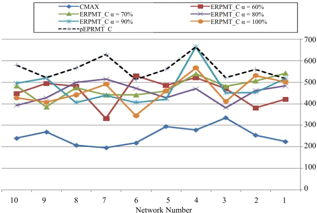
Figure 10 shows results of the same experiments, but

we used ERPMT based on CMAX (pERPMT_C). The same conclusions appl

MAX is less affected to changes of the values of α, and that is because the stability of the CMAX heuristic.

Table 1 depicts the percentage difference in lifetime

between OML, ERPMT_O, and pERPMT_O in different cases, by using Equation (8). Note that, if the res

gative then there is a reduction in lifetime, otherwise, it is an improvement. The enhancement of lifetime for the pERPMT_O is better than OML by 79% and 67% for ERPMT_O for cases when  .





tic. It is obvious that when applying our pER he lifetime has increased in all cases.

The same o





Percentage Difference

Avg.ERPMT _ O vg.OML

 A 100% (8)

Avg.ERPMT _ O 

For Table 2, it depicts the percentage diffe

lifetime between CMAX, ERPMT_C, and pERPMT_ The enhancement of lifetime for the pERPMT_C is

picted in Figure 8. As rence in

C. e conclude that the CMAX has less lifetimes than

OML.

OML

ERPMT_O α = 30% pEPRMT_O

ERPM ERPM

T_O T_O

α = 10% α = 40%

ERPMT_O α = 20% ERPMT_O α = 50%

2000

1800

1600

1400

1200

1000

800

600

400

200

0 10 9 8 7 6 5 4 3 2 1

Network Number

N

etw

or

k A

ver

ag

e

L

if

etim

[image:6.595.145.449.474.714.2]

e

(7)

CMAX

ERPMT_0 α = 30% pEPRMT_C

ERPMT_0 α = 50% ERPMT_0 α = 20%

ERPMT_0 α = 40% ERPMT_0 α = 10%

800 700 600 500 400 300 200 100 0 10 9 8 7 6 5 4 3 2 1

Network Number

N

etw

or

k A

ver

ag

e

L

if

etim

e

[image:7.595.149.444.84.248.2]



αβ



.

Figure 8. Average lifetime routing for CMAX and ERPMT_C

ERPMT_O_H where α = 60% ERPMT_O_H where α = 90% Peprmt_O

2500

2000

1500

1000

500

0 10 9 8 7 6 5 4 3 2 1

Network Number

N

et

w

or

k A

ver

ag

e

L

if

etim

e

ERPMT_O_H where α = 70% ERPMT_O_H where α = 100%

[image:7.595.146.450.283.462.2]

ERPMT_O_H where α = 80% OML_H

Figure 9. Average lifetime routing for OML and ERPMT_O



α β



.

CMAX ERPMT_C α = 70% ERPMT_C α = 90% pEPRMT C

700

600

500

400

300

200

100

0 10 9 8 7 6 5 4 3 2 1

Network Number

N

etw

or

k A

ver

ag

e

L

if

etim

e

ERPMT_C α = 60% ERPMT_C α = 80%

Figure 10. Average lifetime routing for CMAX and ERPMT_C ERPMT_C α = 100%

[image:7.595.125.442.497.710.2]

(8)

better than CMAX by 61% n

  , pERPMT significan y outperform OML and tl 61% and 79% respectively. For

and 45% for ERPMT_O for

CMAX by  

  . , it

more power dedicated for other nodes data -

han it is own data. Through an ve

on runs using OML and CMAX i ly

we read the energy values on

hroughout the lifetime of WS a

de with an ope away fr nd

e total numb of nodes. he

WSN ends because of the de s

one hop aw the sink. And d

PMT we shi d the burde he

ated data, to e node i.e.

means mission t simulati where nodes t sensor no

m is th life of that are the pER aggreg

N l

trans exhausti

ndividual

,Nm

 hop

i

N is sensor a lude that t of the node

n we use rding t middle (

1, 2, N N N, where om the We conc

pletion whe n of forwa s in the ih

er

ay from fte th

1 Nm1

as well as cases whe

[image:8.595.97.498.295.364.2]

The percentage differences in lifetime between OML, ERPMT_O, and pERPMT_O show an enhancement of lifetime for the pERPMT_O over OML by 76% and 61% for ERPMT_O for case when  as depicted in Ta-ble 3.

Table 4 depicts the percentage difference in lifetime

between CMAX, ERPMT_C, and pERPMT_C. The enhancement of lifetime for the pERPMT_C is better than CMAX by 47% and for ERPMT_C is 46% when  .

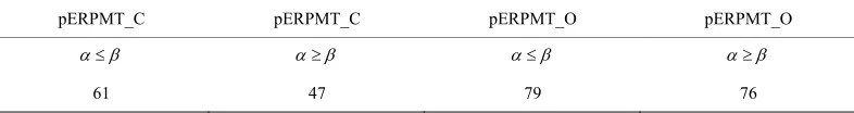
Based on the previous results, Table 5 shows the en-

hancement of the proposed heuristics pERPMT for the

cases of and  

CM

  for the two well known

heuristics, OML and AX. It is evident that when

, where is the hop co k),

g t has high pri

Table 1. The percentage difference between OML and proposed heuristics for

l hat

unt from th ority.

e sin usin Pi



α β. ERPMT_O

Technique OML pERPMT_O

α = 50 α = 40 α = 30 α = 20 α = 10

Avg. life time 348.17 1654.47 878.68 840.58 1128.92 1205.58 1342

%Diff. 0 79 61 59 69 71 64

Table 2. The percentage difference between CMAX and proposed heuristics for αβ. ERPMT_C

Technique CMAX pERPMT_C

α = 50 α = 40 α= 30 α = 20 α = 10

Avg. life time 251.41 640.35 471.27 483.65 442.54 458.08 448.68

[image:8.595.95.498.358.736.2]

%Diff. 0 61 47 48 43 45 44

Table 3. The percentage difference between OML and proposed heuristics for αβ. ERPMT_O

Technique OML pERPMT_O

α= 100 α = 90 α = 80 α = 70 α = 60

Avg. life time 346.17 1448.5857 887.77143 885.64288 8 .58571 929.27143 88144 .8

%Diff. 0 76 61 61 59 63 61

[image:8.595.100.498.583.657.2]

The pe di ween CMAX and propos s for αβ.

Table 4. rcentage fference bet ed heuristic

ERPMT_C

T CMAX pERPM

α = 100 α

echnique T_C

= 90 α = 80 α = 70 α = 60

Avg. life time 251.41 477.6 458.3 477.6 452.74 474.77 456.31

%Diff. 0 47 45 47 44 47 45

Tab Perfo ERPMT vs. CMAX an

pERPMT_C pERPMT_C ERP T_O

le 5. rmance of p d OML.

p MT_O pERPM

      

61 47 79 76

[image:8.595.102.495.683.735.2]

(9)

Table 2 shows t

with α > β. ERPM

of α = 60%. As α increase, we notice a decrease in the

lifetime. OM ette ERP = 70%.

As α increase more decrease in the network lifetime.

6. Conclusions and Future Work

SN play an important role for various applications such as but not limited

control, and nondestructive testing. Since WSN is usually deployed randomly and in a hard to reach areas, limited

battery capac esea nce etwo

lifetime. Many researchers proposed routing techniques t

prolong the e. per, icient pr

ority routing po anagem t heuristics been

proposed and analyzed (pERPMT). Various performing metric parameters have been eva

the pEPRMT outperformed existing routing heuristics in

the literature such nd CMAX by 4%

on average, respectively. This is especially true when he percentage difference for ERPMT T is 18.3% better than OML for case

L is 17.9 b r than MT with α

W

to volcano eruption mentoring, border

ity raises r rcher co rns on the n rk o

WSN lifetim In this pa an eff

i-wer m en have bas

luated. It is observed that

as OML a 77% and 5

  . It is evident that WSN lifetime can be prolonged we shift data aggr tion re-transmission e sink o

ension of plan to look at if

n

ega to th

de to one of the intermediate nodes, given that at least you can find one node in the transmission range of the sink. Otherwise, one of the nodes that are one hope away from the sink is used.

We believe that additional investigation is needed to consider the locality of sensor nodes that depends on the deployment process. Furthermore, the dim

ployment should be taken into account. We

different distributions of sensor nodes as well as movable sink node.

REFERENCES

[1] W. Wilson and G. Atkinson, “Wireless Sensors for Space Applications,” Sensors & Tranducers Journal, Vol. 13, Spe- cial Issue, 2011, pp. 1-9.

[2] I. F. Akyildiz, W. Su, Y. Sankarasubramaniam and F. Ca- yirci, “Wireless Sensor Networks: A Survey, Computer Networks,” Computer Networks, Vol. 38, No. 4, 2002, pp. 393-422. doi:10.1016/S1389-1286(01)00302-4

[3] J. N. AL-Karaki and A. E. Kamal, “Routing Techniques in Wireless Sensor Networks: A Survey,” IEEE Wireless Communications, Vol. 11, No. 6, 2004, pp. 6-28.

[4] F. L. Lewis, “Wireless Sensor Networks, Smart Environ- ments: Technology, Protocols, and Applications,” In: D. J. Cook and S. K. Das, Eds., Smart Environments: Tech- nologies, Protocols, and Applications, John Wiley, New York, 2004. doi:10.1002/047168659X

[5]

S. Lee, lysis of Energy ission and Multi-Hop Trans- mission for Wireless Sensor Networks,” 3rd International IEEE Co Signal-Image Technologies and

Inter-007, pp. 0.

a un ey uting Proto-

c or Wirele ensor Ne rks,” E ier Computer

Networks Journ Vol. 38, N , -422. Wireless

Proceedings of 2004 Inter- nationalCon onWirelessNetworks (ICWN 2004),

Las Vega e 2004, pp. 227-233.

araeh san an , “An Efficient Rout-

ing ique e Lif d Cover-

a Wire nsor s,” nternational

C ence on ital Info ion an ommunication

Te lications DICTAP ok,16-18

[10] M. Alqbilat, “An Efficient Power Management Heuristic

izes The Pow ption of Wireless

Sensor Networks,” Master Thesis, The University of Jor- dan Library, Amman, 2010.

[11] O. Ozdemir, R. Niu, P. K. Var y, A. L. Drozd and R.

o, Vol. 8064, 2011, pp. 806406-806406-11. [12] A. Misra and S. Banerjee, “MRPC: Maximizing Network

Lifetime for R ess Environments,”

Proceedings o mmunications and

V. Lakshma and L. Tassiulas,

J. Lei, R. Yates and L. Greenstein, “A Generic Model for Optimizing Single-Hop Transmission Policy of Replen- ishable Sensor,” IEEE Transactions on Wireless Commu-nications, Vol. 8, No. 2, 2009, p. 54.

Loe, “Feature Aided Probabilistic Data Association Filter for Ballistic Missile Tracking,” Proceedings of the SPIE, Orland

[6] J. Wang, Y. Niu, J. Cho and “Ana

Consumption in Direct Transm

nference on net-Based System

275-28 , Shanghai, 16-18 December 2

[7] K. Akkay and M. Yo is, “A Surv on Ro

ols f ss S

al, twoo. 4, 2003 pp. 393lsev [8] D. Chen and P. K. Varshney, “QoS Support in

Sensor Networks: A Survey,”

ference

s, 21-24 Jun

[9] S. Al-Sh , R. Ha d I. Salah

Techn

ge of less SeThat Maximizes thNetwork 2etime annd I onfer

chnology and Dig It’s App

rmat

(

d C

), Bangk May 2012, pp. 13-18.

That Minim er Consum

shne

eliable Routing in Wirel

f the IEEE Wireless Co

Networking Conference, Orlando, March 2002, pp. 800- 806.

[13] K. Kar, M. Kodialam, T.

“Routing for Network Capacity Maximization in Energy- Constrained Ad-Hoc Networks,” IEEE Societies of the

22nd Annual JointConference of the IEEE Computer and Communications, San Franciso, 30 March-3 April 2003, pp. 673-681.

[14] I. Stojmenovic and X. Lin, “Power-Aware Localized Rout- ing in Wireless Networks,” IEEE Transactions on Parallel and Distributed Systems, Vol. 12, No. 11, 2001, pp. 1122- 1133. doi:10.1109/71.969123

[15] J. Park and S. Sahni, “An Online Heuristic For Maximum Lifetime Routing in Wireless Sensor Networks,” IEEE Transactions on Computer Journal, Vol. 55, No. 8, 2006, pp. 1048-1056. doi:10.1109/TC.2006.116

[16] S. H. Al-Sharaeh, A. Sharieh, A. Abu Dalhoum, R. Hosny and F. Mohammed, “Multi-Dimensional Poisson Distri-bution Heuristic for Maximum Lifetime Routing in Wire- less Sensor Network,” World Applied Sciences Journal, Vol. 5, No. 2, 2008, pp. 119-131.