Title
Effective Community Search over Large Spatial Graphs
Author(s)
FANG, Y; Cheng, CK; LUO, S; HU, J; LI, X
Citation
Proceedings of the 43rd International Conference on Very Large
Data Bases, Munich, Germany, 28 August - 1 September 2017. In
Proceedings of the VLDB Endowment (PVLDB), 2017, v. 10 n. 6,
p. 709-720
Issued Date
2017
URL
http://hdl.handle.net/10722/243528
Rights
Proceedings of the VLDB Endowment (PVLDB). Copyright ©
Very Large Data Base (VLDB) Endowment Inc.; This work is
licensed under a Creative Commons
Effective Community Search over Large Spatial Graphs
Yixiang Fang, Reynold Cheng, Xiaodong Li, Siqiang Luo, Jiafeng Hu
Department of Computer Science, The University of Hong Kong, Hong Kong {yxfang, ckcheng, xdli, sqluo, jhu}@cs.hku.hk
ABSTRACT
Communities are prevalent in social networks, knowledge graphs, and biological networks. Recently, the topic of community search (CS) has received plenty of attention. Given a query vertex, CS looks for a dense subgraph that contains it. Existing CS solutions do not consider the spatial extent of a community. They can yield communities whose locations of vertices span large areas. In applications that facilitate the creation of social events (e.g., finding conference attendees to join a dinner), it is important to find groups of people who are physically close to each other. In this situation, it is desirable to have aspatial-aware community(or SAC), whose vertices are close structurally and spatially. Given a graphGand a query vertexq, we develop exact solutions for finding an SAC that containsq. Since these solutions cannot scale to large datasets, we have further designed three approximation algorithms to compute an SAC. We have performed an experimental evaluation for these solutions on both large real and synthetic datasets. Experimental results show that SAC is better than the communities returned by existing solutions. Moreover, our approximation solutions can find SACs accurately and efficiently.
1.
INTRODUCTION
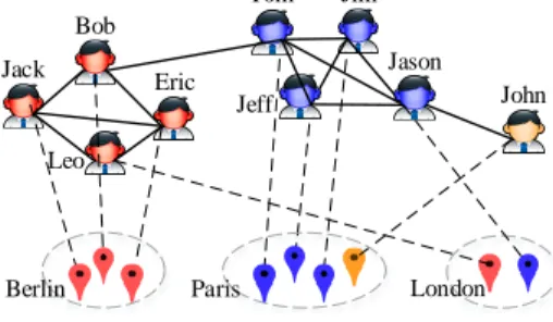
With the emergence of geo-social networks, such as Twitter and Foursquare, the topic of geo-social networks has gained a lot of attention [1, 30, 26, 12]. In these networks, a user is often associated with location information (e.g., positions of her hometown and check-ins). These networks are collectively known asspatial graphs. Figure 1 depicts a spatial graph with nine users in three cities Berlin, Paris, London, and each user has a specific location. The solid lines represent their social relationship, and the dashed lines denote their hometown locations.
In this paper, we study the problem of performing online community search (CS) on spatial graphs. Given a spatial graph
Gand a vertexq∈G, our goal is to find a subgraph ofG, called
aspatial-aware community(or SAC). Essentially, a community is
a social unit of any size that shares common values, or that is situated in a close area [22]. An SAC is such a community with highstructure cohesivenessandspatial cohesiveness. The structure
This work is licensed under the Creative Commons Attribution-NonCommercial-NoDerivatives 4.0 International License. To view a copy of this license, visit http://creativecommons.org/licenses/by-nc-nd/4.0/. For any use beyond those covered by this license, obtain permission by emailing [email protected].
Proceedings of the VLDB Endowment,Vol. 10, No. 6 Copyright 2017 VLDB Endowment 2150-8097/17/02. Jack Bob Tom Jim Jason John Eric Leo
City1 City2 City3
Jeff Jack Bob Tom Jim Jason John Eric Leo
Berlin Paris London
Jeff
Figure 1: A geo-social network.
cohesiveness mainly measures the social connections within the community, while the spatial cohesiveness focuses on the closeness among their geo-locations. Figure 1 illustrates an SAC with three users{Tom,Jeff,Jim}, in which each user is linked with each other and all of them are inParis.
Table 1: Works on community retrieval.
Graph Type Community Detection (CD) Community Search (CS) Non-spatial [25, 14] [29, 7, 6, 21, 19, 11] Spatial [16, 10, 4] SAC search
Prior works. The community retrieval methods can generally be classified into community detection (CD) and community
search (CS), as shown in Table 1. Earlier CD methods [25,
14] mainly focus on link analysis without considering spatial features. Some recent studies [2] have shown that, in networks where vertices occupy positions in an Euclidian space, spatial constraints may have a strong effect on their relationship patterns, so some works [16, 10, 4] have considered the spatial features for community detection. All these CD methods often detect all the communities from an entire graph using some predefined global criteria (e.g., modularity [20]), so their focus is beyond personalized community search. Also, their efficiency is inadequate for fast and online community retrieval since they require to enumerate all the communities. To address these limitations, some works [29, 7, 6, 19, 11] focus on online
community search, a query-dependent variant of community detection, and they are able to find communities for a specific vertex. However, almost all these CS works focus on link analysis and do not consider the spatial features. In Figure 1, for example, previous CS methods [29, 7] tend to putJasonandTom,Jeff,
Jim into the same community, although Jason is located in another cityLondon. This community may not be very useful
2016/6/9 Circles
file:///C:/Users/Admin/Dropbox/SAC%20search/workspace/sac/info/1064.html 1/1 B
A
Map data ©2016 Google
(a)user1’s SACs (b)user2’s SACs
Figure 2: SACs in Brightkite dataset.
for some location-based services (e.g., setting up events). To alleviate this issue, in this paper we study SAC search which finds communities for a particular query vertex in an “online” manner. Our later experimental results on real datasets show that, the communities found by our methods are often in a much smaller areas than that of previous CS methods, i.e., the radii of the spatial circles covering communities found by [29] and [7] are 50 and 20 times larger than those of SAC search.
SAC search. We now discuss how to measure the structure cohesiveness and spatial cohesiveness of an SAC. We adopt the commonly used metricminimum degree[29, 7, 21] to measure the structure cohesiveness. Note that in our method, the minimum degree metric can be easily replaced by other metrics like
k-truss [19] andk-clique [6]. To measure the spatial cohesiveness, we consider thespatial circle, which contains all the community members. In particular, given a query vertexq∈G, our goal is to find an SAC containingqin the smallestminimum covering circle
(or MCC) and all the vertices of the SAC satisfy the minimum degree metric. The main features of SAC search are summarized as follows.
• Adaptability to location changes. In geo-social networks (e.g., Brightkite and Foursquare), a user’s location often changes frequently, due to its nature of mobility. As a result, users’ spatially close communities change frequently as well. Let us consider two real examples in Brightkite, which once was a popular location-based social networking website. Figure 2(a) shows a user’s two SACs in two consecutive days, when she moves from place “A” to place “B” in US, in which each SAC is located in an MCC denoted by a circle. Note that all the members are different except the user itself. Figure 2(b) shows another user’s two SACs in three days, when she moves from place “C” to place “D”. These real examples clearly show that a user’s communities could evolve over time. In our later experiments, we find that for two SACs with time gap of six hours or more, the average Jaccard similarity of these two community member sets decreases by 25%.
Moreover, the link relationship also evolves over time. So the existing CD methods may easily lose the freshness and effectiveness after a short period of time. On the contrary, our SAC search can adapt to such dynamic easily, as it can answer queries in an “online” manner. Also, our methods do not rely on any offline computation, such as graph clustering or index structures.
• Personalization. SAC search allows a query user to find a community that exhibits both high structure cohesiveness and spatial cohesiveness. The parameter k, the minimum degree, allows the user to control the strength of link intensiveness. For example, SAC search can answer queries such as who are my
nearby friends so that we can form a particular club? In contrast, existing CD methods [16, 10, 4] often use some global criteria (e.g., modularity), and consider thestaticcommunity detection problem, where the graph is partitioned a-priori with no reference to the particular query vertices.
• Online search. Similar to other online CS methods, our method is able to find an SAC from a large spatial graph quickly once a query request arrives. However, existing CD methods for spatial graphs, are generally slower, as they are often designed for generating all the communities for an entire graph.
Applications.We now discuss the applications of SAC search.
•Event recommendation.Emerging geo-social applications such asMeetup1,Meetin2, andEventbrite3 allow social network users to meet physically for various interesting purposes (e.g., party, dinner, and dating). For example,Meetuptracks its users’ mobile phone locations, and suggests interesting location-based events to them [30]. Suppose thatMeetupwishes to recommend an event to a user u. Then we can first find u’s SAC, whose members are physically close tou. Events proposed byu’s SAC member
v can then be introduced to u, so that u can meet v if she is interested inv’s activity. Sinceu’s location changes constantly,
u’s recommendation needs to be updated accordingly. Also, these applications often have to handle requests from a large number of online users efficiently. Our high-performance SAC search algorithms can therefore benefit these applications.
•Social marketing. As studied in [23], people with close social relationships tend to purchase in places that are also physically close. To boost sales figures, advertisement messages can be sent to the SACs of users who bought similar products before. For instance, if uhas bought an item, the system can advertise this item tou’s SAC members.
• Geo-social data analysis. A common data analysis task is to study features about geographical regions. As discussed in [5], these features are often related to the people located there. For example, Silicon Valley can be characterized by “information technology” because many residents/workers there are interested in this topic. Hence, by analyzing members of an SAC, it is possible to better understand the characteristics of a geographical area. As also discussed in [27] and Figure 2, SAC search can be used to monitor and analyze the movement of communities. We can thus track the evolution and composition ofu’s SAC as she moves.
Challenges and contributions.The SAC search problem is very challenging, because the center and radius of the smallest MCC containingqare unknown. A basic exact approach takesO(m×
n3)time to answer a query, wherenandmdenote the numbers of vertices and edges inG. This is very costly, and is impractical for large spatial graphs with millions of vertices. So we turn to develop efficient approximation algorithms, which are able to find an SAC in an MCC of similar size with the smallest MCC. We first develop a basic approximation algorithmAppInc, which achieves an approximation of 2. Here, the approximation ratio is defined as the ratio of the radius of MCC returned over that of the optimal solution. Inspired byAppInc, we develop another approximation algorithmAppFast, which is faster and also has a more flexible approximation ratio, i.e.,2 +F, whereF is an arbitrary small non-negative value. However, AppInc and AppFast cannot achieve even better accuracy with an approximation ratio less than 2. To tackle this issue, we further propose another approximation algorithmAppAccwith an approximation ratio of1 +A, where
1 https://www.meetup.com/ 2 https://www.meetin.org/ 3 https://www.eventbrite.hk/
710
0< A <1. Overall, these approximation algorithms theoretically guarantee that, the radius of the MCC containing the SAC found has an arbitrary expected approximation ratio. Finally, inspired by the design of approximation algorithms, we develop an advanced exact algorithmExact+, and our later experiments show that it is four orders of magnitude faster than the basic exact algorithm.
We have implemented our algorithms and performed extensive experiments on four real datasets and two synthetic datasets. We develop several metrics to measure the quality of a community, considering the spatial circles and distances among community members, and compare existing CD and CS methods under these metrics. These results confirm the superiority of SAC search. In addition, we also have run experiments on a dynamic spatial graph, where users’ locations change frequently, and the results show that SAC search can well adapt to location changes.
We further evaluate the efficiency of SAC search, and the results show that the developed algorithms are more efficient than the baseline algorithms. From extensive experiments, we conclude that, for moderate-size graphs,Exact+is the best choice, as it achieves the highest quality with reasonable efficiency, while for large graphs with millions of vertices,AppFastandAppAccare better choices as they are much faster thanExact+.
Organization. We review the related work in Section 2. We formally define the problem studied in this paper in Section 3. Section 4 presents the proposed query algorithms. We report the experimental results in Section 5. Section 6 concludes this work.
2.
RELATED WORK
Community detection (CD).Discovering communities from a network is a fundamental problem in network science, and it has been widely studied in the past decades. Classical solutions [25, 14] employ link-based analysis to obtain these communities. However, they do not consider the location information. Some recent works [15, 16, 10, 4] focus on identifying communities from spatially constrained graphs, whose vertices are associated with spatial coordinates [2]. For example, a geo-community [15] is like a community which is a graph of intensely connected vertices being loosely connected with others, but it is more compact in space. Guo et al. [16] proposed the average linkage (ALK) measure for clustering objects in spatially constrained graphs. In [10], Expert et al. uncovered communities from spatial graphs based on modularity maximization. In [4], Chen et al. proposed an algorithm based on fast modularity maximization for detecting communities from spatially constrained networks. We will compare it with our methods in experiments. The differences of CD algorithms and our SAC search are three-fold. First, CD algorithms are generally costly and time-consuming, as they often detect all the communities from an entire network. Second, it is not clear how they can be adapted for online community retrieval. Third, as pointed out by [20], the modularity based methods [10, 4] often fail to resolve small-size communities, even when they are well defined. In this paper, we propose online algorithms for finding SACs from large spatial graphs.
Community search (CS). In recent years, there is another related but different problem of community detection, called community search. The goal of community search is to obtain communities in an “online” manner, based on a query request. For example, given a vertexq, several existing works [29, 7, 6, 21, 19] have proposed effective algorithms to obtain the most likely community that contains q. The minimum degree
metric is often used to measure the structure cohesiveness of a community [29, 7]. In [29], Sozio et al. proposed the first algorithmGlobal to find thek-cored containingq. In [7], Cui
Table 2: Notations and meanings.
Notation Meaning
G(V, E) a graph with vertex setV and edge setE n,m the sizes of vertex and edge setsV andEresp.
G[S] a subgraph ofGinduced by vertex setS nb(v) the neighbor set of vertexvinG degG(v) the degree of vertexvinG
G0⊆G G0is a subgraph ofG
O(o, r) a circle with centeroand radiusr
|u, v| the Euclidean distance from verticesutov Ψ Results ofExactandExact+
Φ,Λ,Γ Results ofAppInc,AppFast,AppAccresp.
et al. proposed a more efficient algorithm Local, which uses local expansion techniques to boost the query performance. We will compare these two solutions in our experiments. In addition, some recent works [21, 11] also use the minimum degree metric to search communities from attributed graphs. Other well known structure cohesiveness metrics, includingk-clique [6],k-truss [19] and connectivity [18], have also been considered for online community search. But these works assume non-spatial graphs, and overlook the locations of vertices. Thus, it is desirable to design algorithms for searching communities from spatial graphs.
3.
PROBLEM DEFINITION
Data Model.We consider a geo-social network graphG(V, E), which is an undirected graph with vertex set V and edge set
E, where vertices represent entities and edges denote their relationships. For each vertexv ∈ V, it has a location position (v.x, v.y), wherev.x andv.y denote its positions alongx- and
y-axis in a two-dimensional space. Note that our methods can be easily applied to multi-dimensional space. Letn and mbe the corresponding sizes ofV andE. We illustrate the data model using Example 1. Table 2 shows the notations used in this paper.
EXAMPLE 1. Figure 3(a) depicts a geo-social network
containing 10 vertices{Q, A, B,· · ·, I}. The solid lines linking the vertices are the edges, denoting their social relationships.
4 2 6 0 8 2 4 6 Q A B D C 0 x y E F G H I Q A B D C E F G H I 3 2 1 4 2 6 0 8 2 4 6 Q A B D C 0 x y F G H I 4 2 6 0 8 2 4 6 Q A B D C 0 x y E F G H I Q A B D C E F G H I 4 2 6 0 8 2 4 6 Q A B C D 0 x y E F G H I 3 2 1 2-approximation 4-approximation Lemma 1: 0.5d0≤ ropt≤ r0 Corollary 1: d0≥ r0
Lemma 2: 0.5r0≤ ropt≤ r0, the incremental solution is 2-approximated.
Lemma 3: the optimal solution is in O(Q, 2r0).
Corollary 2: any solution in O(Q, 2r0) is a 4-approximated.
Lemma 4: in the optimal solution, at least one fixed vertex having
distance to q is in range [d0, 2r0].
Lemma 5: in the optimal solution, at least one fixed vertex having
distance to q is in range [0, d0]
(a) spatial graph (b)k-core decomposition
Figure 3: An example of geo-social network.
Spatial-aware community (SAC).Conceptually, an SAC is a subgraph,G0, of the graphGsatisfying: (1)Connectivity: G0 is connected; (2)Structure cohesiveness: all the vertices in G0 are linked intensively; and (3)Spatial cohesiveness: all the vertices in
G0are spatially close to each other.
Structure cohesiveness. A well-accepted notion of structure cohesiveness is theminimum degreeof all the vertices that appear in the community is at leastk[29, 28, 3, 7, 21]. This is used in
k-core and our SAC search. Let us discuss thek-core first.
DEFINITION1 (k-CORE[28, 3]). Given an integerk (k ≥
0), thek-core ofG, denoted byHk, is the largest subgraph ofG,
such that∀v∈Hk,degHk(v)≥k.
We say thatHkhas an order ofk. Thecore numberof a vertex
v ∈ V is then defined as the highest order of the k-corethat containsv. Ak-core has some important properties [3]: (1)Hk contains at leastk+ 1vertices; (2)Hk may not be a connected graph; (3)k-cores are nested, i.e.,Hk+1⊆Hk; and (4) Computing
the core numbers of all the vertices in a graph, also known ask-core decomposition, can be completed using a linear algorithm [3].
As a k-core may not be a connected subgraph, we denote its connected components by k-coreds, which are usually the “communities” returned byk-cored search algorithms [29, 7]. In
Example 1, each k-core is covered by an ellipse as shown in Figure 3(b). Note that 2-core has two2-coreds with vertex sets
{Q, A, B, C, D, E}and{F, G, H}respectively.
Remarks.Although we use the minimum degree as the structure cohesiveness metric, our solutions can be easily adapted to other structure cohesiveness criteria likek-truss [19] andk-clique [6].
Spatial cohesiveness. In this paper, to ensure high spatial cohesiveness, we require all the vertices of an SAC in a minimum covering circle (MCC) with the smallest radius. In the literature [8, 9, 24, 17], the notion of MCC has been widely adopted to achieve high spatial compactness for a set of spatial objects. The MCC and SAC search are defined as follows.
DEFINITION2 (MCC). Given a set of verticesS, the MCC
ofSis the spatial circle, which contains all the vertices inSwith the smallest radius.
PROBLEM1 (SACSEARCH). Given a graphG, a positive
integerkand a vertexq ∈ V, return a subgraphGq ⊆ G, and
the following properties hold:
1.Connectivity.Gqis connected and containsq;
2.Structure cohesiveness.∀v∈Gq,degGq(v)≥k;
3. Spatial cohesiveness. The MCC of vertices inGqsatisfying
Properties 1 and 2 has the minimum radius.
We call a subgraph satisfying properties 1 and 2 a feasible
solution, and the subgraph satisfying all the three properties the
optimalsolution (denoted byΨ). We denote the radius of the MCC
containingΨbyropt. Essentially, SAC search finds the SAC in an MCC with the smallest radius among all the feasible solutions. In Example 1, letC1={Q, C, D}and C2={Q, A, B}. The two
circles in Figure 3(a) denote the MCCs ofC1andC2respectively.
Letq=Qandk=2. The optimal solution of this query isG[C1], and
ropt=1.5. Note thatG[C2]andG[C1∪C2]are feasible solutions.
We also consider theθ-SAC search, which returns a community satisfying: properties 1 and 2 of SAC search, and all the vertices are in a spatial circle O(q, θ), where θ is an input parameter. This θ-SAC search is essentially a variant of Global [29] by introducing a parameterθ. Consider the graph in Example 1 with
q=Q,k=2 andθ=3.1.θ-SAC search will returnG[C1∪C2]as the
community, as all of its vertices are inO(Q,3.1).
Theθ-SAC query can be used when a user has some background knowledge (e.g., size of the region containing the SAC, and density of users in the region concerned). However, it can be difficult for a user of an application, such as Meetup, to specify an appropriate value ofθ. As will be discussed in our experiments, the effectiveness ofθ-SAC search is sensitive to θ. If θ is too small, no community can be found; ifθ is too large, then the community is not spatially compact. A casual application user may then have to repeat the query with differentθvalues, before getting
a satisfactory result. For the SAC search, the user does not need to specifyθ; instead, SAC search automatically suggests a community with tight structural and spatial cohesiveness. Thus, SAC search is more convenient to use thanθ-SAC. In the above example, if
θ<2.2, no community is found; ifθ>5.1,G[C3]will be returned,
whereC3={Q, A, B, C, D, E}. In fact, there are more spatially
compact SACs (e.g.,G[C1],G[C2]andG[C1∪C2]), among which
the most compact one (G[C1]) is returned by the SAC search. We
next focus on SAC search.
4.
SAC SEARCH ALGORITHMS
We now present fast SAC search algorithms. Most of our solutions follow the two-step framework: (1) find a community
S of vertices, based on some CS algorithm e.g.,Global [29], and (2) find a subset ofS that satisfies both structure and spatial cohesiveness. Step (2) is computationally challenging; a simple way is to enumerate all the possible subsets ofS, and then choose the one that satisfies the two criteria of SAC. In Example 1, when
q=Qandk=2,S={Q, A, B, C, D, E}; an SAC is then chosen from the 26–1=63 subsets of S. This requires the examination of an exponential number of possible subsets ofS in Step (2). In our experiments, the typical size ofS ranges from1Kto100K. As a result, the performance of SAC search can be seriously affected. Hence, we study polynomial-time SAC search algorithms for Step (2). Later we will also present theAppIncsolution, which does not use Step (1).
Table 3: Overview of algorithms for SAC search.
Algo. Approx. ratio Time complexity
Exact 1 O(m×n3)
AppInc 2 O(mn)
AppFast 2+F(F≥0)
IfF>0,O(m·min{n,log1
F}) IfF=0,O(mn) AppAcc 1+A(0<A<1) O(m2 A ×min{n,log1 A}) Exact+ 1 O(m 2 A ·min{n,log 1 A}+m|F1| 3)
We first present a basic exact algorithmExact, which takes
O(m×n3)
to answer a single query. This is very time-consuming for large graphs. So we turn to design more efficient approximation algorithms. Here, the approximation ratio is defined as the ratio of the radius of MCC returned over that of the optimal solution. Inspired by the approximation algorithms, we also design an advanced exact algorithmExact+, which is at least four orders of magnitude faster than Exact as shown by our experiments. Their approximation ratios and time complexities are summarized in Table 3, whereF andAare parameters specified by the query user. The value|F1|is the number of “fixed vertices”, which will
be defined in Section 4.1;|F1|is often much smaller thann. We
will explain this parameter in more detail. Note that the space cost of each algorithm is linear with the size of graphG.
AppInc is a 2-approximation algorithm, and it is much faster than Exact. Inspired by AppInc, we design another (2+F)-approximation algorithmAppFast, whereF≥0, which is faster thanAppInc. The limitation ofAppIncandAppFast
is that their theoretical approximation ratios are at least 2. To achieve even lower approximation ratio, we further design another algorithmAppAcc, whose approximation ratio is (1+A), where 0<A<1 is a value specified by the query user. It is slightly slower thanAppFast, as it spends more effort on finding more accurate solutions. Overall, these approximation algorithms guarantee that
the radius of the MCC of the community has an arbitrary expected approximation ratio.
All algorithms exceptAppIncfollow the two-step framework. Note that Step (1) of the two-step framework is not necessary for
AppInc, since it works in an incremental manner. In addition, we can observe that, there is a trade-off between the quality of results and efficiency, i.e., algorithms with lower approximation ratios tend to have higher complexities. Our later experiments show that, for moderate-size graphs,Exact+achieves not only the highest quality results, but also reasonable efficiency. While for large graphs with millions of vertices,AppFastandAppAcc
should be better choices as they are much faster thanExact+.
4.1
The Basic Exact Algorithm
As mentioned before, ak-core contains at leastk+ 1vertices. When the inputk=1, we can simply return the subgraph, induced byqand its nearest neighbor, as the result. So in the rest of this paper, we mainly focus on the casek≥2.
We now describe a useful lemma about MCC, described in [9], which inspires the design of our algorithms.
LEMMA 1. [9] Given a setS (|S| ≥ 2) of vertices, its MCC
can be determined by at most three vertices inS which lie on the
boundary of the circle. If it is determined by only two vertices, then the line segment connecting those two vertices must be a diameter of the circle. If it is determined by three vertices, then the triangle consisting of those three vertices is not obtuse.
By Lemma 1, there are at least two or three vertices lying on the boundary of the MCC of the target SAC. We call vertices lying on the boundary of an MCCfixed vertices. So a straightforward method of SAC search can follow the two-step framework directly. It first finds thek-cored containingq, which is the same asGlobal
does, and then returns the subgraph achieving both the structure and spatial cohesiveness by enumerating all the combinations of three vertices in thek-cored. We denote this method byExact.
Algorithm 1 showsExact. It first finds a list X of vertices of thek-cored, and sorts them according to their distances fromqin ascending order (lines 2-3). NoteXidenotesi-th vertex. For each three vertex combination, it verifies whether there is ak-cored in the
MCC fixed by it, and finally returnsΨ(lines 4-14). Algorithm 1Query algorithm:Exact
1: functionEXACT(G,q,k)
2: find the vertex listXof thek-cored containingq;
3: sort vertices ofX; 4: initializer←+∞,Ψ← ∅; 5: fori←3to|X|do 6: forj←1toi–2do 7: forh←j+ 1toi–1do 8: compute the MCCmccof{Xi, Xj, Xh}; 9: ifmcc.radius < rthen 10: R←a set of vertices inmcc; 11: ifexist ak-cored withqinG[R]then
12: r←mcc.radius,Ψ←thisk-cored;
13: if|q, Xi|>2rthenbreak; 14: returnΨ;
In addition, we present another useful lemma, which is about the maximum pair-wise distance for vertices inΨ.
LEMMA 2. [17] The maximum distance between any pair of
vertices,uandvinΨ, is in the range[√3ropt,2ropt].
Complexity. The time complexity of ExactisO(m×n3),
since there are three nested for-loops and finding ak-cored takes linear time costO(m)(we assumem≥n) [3].
4.2
A 2-Approximation Algorithm
The major limitation ofExactis its high computational cost, which makes it impractical for large spatial graphs with millions of vertices. To alleviate this issue, we now develop more efficient approximation algorithms. We first presentAppInc, which has an approximation ratio of 2. Our key observation is that, the optimal solution Ψ is usually very close to q. So we consider the smallest circle, denoted byO(q, δ), which is centered atqand contains a feasible solution, denoted byΦ. Let the radius of the MCC coveringΦbeγ(γ ≤δ). Note that,γcan be obtained by computing the MCC containingΦby a linear algorithm [24]. Then, we have the following two interesting lemmas:
LEMMA 3. 12δ≤ropt≤γ.
PROOF. We haveropt≤γobviously, asΨis the optimal. We prove 1
2δ≤roptby contradiction. Supposeropt< 1
2δ. Since the
MCC ofΨcontainsq, for anyv∈Ψ, we have|v, q| ≤2×ropt. Asropt<12δ, we have|v, q| ≤2×ropt< δ. This implies thatΨ must be in a circle, whose center isqand radius is smaller thanδ. This contradicts the fact that,O(q, δ)is the minimum circle with centerqcontaining a feasible solution. Hence, Lemma 3 holds.
LEMMA 4. The radius of the MCC covering the feasible
solutionΦhas an approximation ratio of 2.
PROOF. LetSbe the set of vertices inO(q, δ). Since the vertex set ofΦis a subset ofS, the MCC ofΦhas a radius no larger than that ofS, i.e.,γ ≤δ. By Lemma 3, we have 12γ ≤ 1
2δ ≤ropt.
This implies that rγ
opt ≤2.0. Hence, Lemma 4 holds.
AppInc finds Φ in an incremental manner. Specifically, it considers vertices close toqone by one incrementally, and checks whether there exists a feasible solution when a new vertex is considered. It stops once a feasible solution has been found. Algorithm 2Query algorithm:AppInc
1: functionAPPINC(G,q,k) 2: initializeQueue,S← ∅,T ← ∅,Φ← ∅; 3: Queue.add(q); 4: while|Queue|>0do 5: p←Queue.poll(); 6: S.add(p); 7: forv∈nb(p)do 8: ifdegG(v)≥kthen 9: if|v, q| ≤ |p, q|then 10: S.add(v); 11: else ifv /∈Tthen
12: Queue.add(v); T.add(v);
13: if|S∩nb(q)| ≥k∧ |S∩nb(p)| ≥kthen 14: ifexist ak-cored containingqinG[S]then
15: Φ←thisk-cored; break; //stop 16: returnΦ;
Algorithm 2 presentsAppInc. First, it initializes four variables
Queue, S, T and Φ: Queue is a priority queue of vertices, in which vertices are sorted in an ascending order according to their distances toq; S is the set maintaining vertices close toq
incrementally;T is a set for recording vertices added toQueue; andΦis the approximated SAC. Then, it addsqtoQueuein the beginning (line 3). In the while loop (lines 4-15), it first gets the nearest vertex,p, fromQueue, and adds it toS(lines 5-6). Next, it considersq’s neighbors (lines 7-12). For each neighborv∈X, if it is inO(q,|p, q|), we add it toSdirectly; otherwise, we put it intoQueueas it is already inO(q,|p, q|). Note that in any feasible solution, each vertex has at leastkneighbors. So if bothpandq
4 2 6 0 8 2 4 6 Q A B C D 0 x y E F G H I r1 r2 u l r δ ≤α Q 4 2 6 0 8 2 4 6 Q A B C D 0 x y E F G H I γ δ l u q r δ l u q r δ 4 2 6 0 8 2 4 6 q 0 x y γ β rmin ropt o β c β o c r+ r -f 4 2 6 0 8 2 4 6 Q A B C D 0 x y E F G H I r1 r2 r3
Figure 4:IllustratingAppInc.
4 2 6 0 8 2 4 6 Q A B C D 0 x y E F G H I r1 r2 u l r δ ≤α Q 4 2 6 0 8 2 4 6 Q A B C D 0 x y E F G H I γ δ 2γ l u q r δ l u q r δ 4 2 6 0 8 2 4 6 q 0 x y γ β rmin ropt o β c β o c r+ r -f 4 2 6 0 8 2 4 6 Q A B C D 0 x y E F G H I r1 r2 r3
Figure 5:IllustratingAppFast.
have at leastk neighbors inS, it checks whether there exists an SAC inG[S]. If it exists, thenAppIncreturns it (lines 13-16).
We illustrateAppIncusing Example 2.
EXAMPLE 2. In Example 1, letq=Qandk=2. AppIncfirst
addsAtoSand no SAC can be found. Then, it addsBtoS, finds
Φwith members set{Q, A, B}. Soγ=1.803 andδ=|Q, B|=2.24. The actual approximation ratio is 1.803/1.5=1.202.
COROLLARY 1. If q is the center of the MCC covering Ψ,
AppIncfinds the optimal solution, i.e.,Φequals toΨ.
PROOF. This can be proved directly by contradiction.
COROLLARY 2. The optimal solutionΨis inO(q,2γ).
PROOF. By Lemma 3, we haveropt≤γ. This implies that, for anyv∈Ψ, we have|q, v| ≤2×γ. Thus, all the vertices ofΨare inO(q,2γ), and Corollary 2 holds.
Complexity. InAppInc, the while loop is executed at mostn
times, and each takesO(m), as computingk-cored takesO(m). So
the total time cost ofAppIncisO(mn).
4.3
A (2+
F)-Approximation Algorithm
Although AppInc is much faster than Exact, it is still inefficient for large graphs, since its time complexity is quadratic. In this section, we propose another fast approximation algorithm, calledAppFast, which has a more flexible approximation ratio, i.e.,2 +F, whereFis an arbitrary non-negative value.Instead of finding the circleO(q, δ)in an incremental manner,
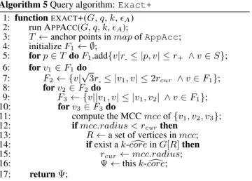
AppFastapproximates the radiusδby performing binary search. This is based on the observation that, the lower and upper bounds ofδ, denoted bylandu, are stated by Eq (1):
l= max
v∈KN N(q)|q, v|, u= maxv∈X|q, v|, (1) whereX is the list of vertices of thek-cored containingq, and
KN N(q)contains theknearest vertices inX∩nb(q)toq. Hence, we can approximate the radius of the circleO(q, δ)by performing binary search within[l, u].
Algorithm 3 presentsAppFast. We denote the SAC returned byAppFastbyΛ. F is an input parameter. By following the two-step framework, it first computes thek-cored (line 2), and then
findsΛfrom thek-cored (lines 3-14). Some variables such asΛ,
landuare initialized (line 3). In while loop (lines 4-14), it first finds an SACΛ0fromO(q, r)using breadth first search (BFS). If Λ0 does exist, it first updatesΛ, since this solution has a smaller radius. It then checks whether the gap, i.e.,r−l, is smaller thanα
(we will discuss how to set this gap later). If it is not larger thanα, then it returnsΛ; otherwise, it updatesuas the maximum distance fromqto vertices inΛ, which ensures that the feasible solution found later has at least one less vertex thanΛ. IfΛ0does not exist,
Algorithm 3Query algorithm:AppFast
1: functionAPPFAST(G,q,k,F)
2: find the vertex listXof thek-cored,Λ, containingq; 3: initializel,uusing Eq (1);
4: whileu > ldo 5: r←l+u
2 ;
6: S←vertices inO(q, r);
7: Λ0←thek-cored containingqinG[S]; 8: ifΛ06=∅then 9: Λ←Λ0; 10: ifr−l≤αthen returnΛ; 11: u←max v∈Λ|q, v|; 12: else 13: ifu−r≤αthen returnΛ; 14: l← min v∈Λ∧v /∈S|q, v|;
it returnsΛif the gap, i.e.,u−r, is small enough; otherwise, it updateslas the minimum distance fromqto vertices inΛ, but not inS, which ensures that the setS in the next iteration has at least one more vertex than currentS.
We illustrateAppFastusing Example 3.
EXAMPLE 3. In Figure 5 (q=Q,k=2,F=0.1),AppFastfirst
initializesl=2.24,u=5.10, and tries to find a feasible solution from
O(Q, r1)andO(Q, r2), wherer1=3.67 andr2=2.24. It stops after searchingO(Q, r2), asr2−l=0.Λis the same withΦ.
LEMMA 5. In AppFast, the radius of the MCC coveringΛ
has an approximation ratio of (2 +F), ifαis set asr2+×F
F.
PROOF. Consider the last loop in Algorithm 3 when returning Λ. Let the gap between the radii, which result in a feasible solution and no solution, beα.
If Λ0 does exist (lines 8-10), the returned Λ is contained in
O(q, r). We havel≤δ≤r≤uandr−l≤α(see Figure 6(a)). So we haver≤δ+α.
IfΛ0does not exist (lines 12-13), the returnedΛis contained in
O(q, u). We havel≤r≤δ≤uandu−r≤α(see Figure 6(b)). So we haver≤δ+α.
Therefore, we always haver≤δ+α. We denote the radius of the MCC coveringΛbyrΛ. Considering Lemma 3, we have
rΛ≤r≤2ropt+α. (2)
Eq (2) also implies that,ropt≥ 12(r−α). Then, rΛ ropt ≤ 2ropt+α ropt = 2 + α ropt ≤2 + 2α r−α. (3) Letr2−αα≤F, then we haverrΛ
opt ≤2 +F, ifαis set as
r×F
2+F.
Hence, Lemma 5 holds.
4
2
6
0
8
2
4
6
Q
A
D
C
B
0
x
y
Lemma 1: 0.5d
0≤
r
opt≤
r
0Corollary 1: d
0≥
r
0Lemma 2: 0.5r
0≤
r
opt≤
r
0, the incremental solution is 2-approximated.
Lemma 3: the optimal solution is in O(Q, 2r
0).
Corollary 2: any solution in O(Q, 2r
0) is a 4-approximated.
Lemma 4: in the optimal solution, at least one fixed vertex having
distance to q is in range [d
0, 2r
0].
Lemma 5: in the optimal solution, at least one fixed vertex having
distance to q is in range [0, d
0]
4
2
6
0
8
2
4
6
Q
A
B
C
D
0
x
y
E
F
G
H
I
r
1r
3r
2u
l
r
δ
≤α
Q
4
2
6
0
8
2
4
6
Q
A
B
C
D
0
x
y
E
F
G
H
I
γ
δ
2γ
4
2
6
0
8
2
4
6
Q
0
x
y
γ
β
r
minr
opto
β
c
l
u
q
r
δ
l
u
q
r
δ
4
2
6
0
8
2
4
6
Q
A
D
C
B
0
x
y
Lemma 1: 0.5d
0≤
r
opt≤
r
0Corollary 1: d
0≥
r
0Lemma 2: 0.5r
0≤
r
opt≤
r
0, the incremental solution is 2-approximated.
Lemma 3: the optimal solution is in O(Q, 2r
0).
Corollary 2: any solution in O(Q, 2r
0) is a 4-approximated.
Lemma 4: in the optimal solution, at least one fixed vertex having
distance to q is in range [d
0, 2r
0].
Lemma 5: in the optimal solution, at least one fixed vertex having
distance to q is in range [0, d
0]
4
2
6
0
8
2
4
6
Q
A
B
C
D
0
x
y
E
F
G
H
I
r
1r
3r
2u
l
r
δ
≤α
Q
4
2
6
0
8
2
4
6
Q
A
B
C
D
0
x
y
E
F
G
H
I
γ
δ
2γ
4
2
6
0
8
2
4
6
Q
0
x
y
γ
β
r
minr
opto
β
c
l
u
q
r
δ
l
u
q
r
δ
(a)Λis inO(q, r) (b)Λis inO(q, u)
Figure 6: Illustrating the proof of Lemma 5.
Remark:IfF=0, the returned communityΛis the same asΦ.
COROLLARY 3. The optimal solutionΨis inO(q,2rΛ), where
rΛis the radius of the MCC containingΛinAppFast.
PROOF. Since we haveropt ≤ rΛ, for anyv ∈ Ψ, we have
|q, v| ≤2×rΛ. Thus, all the vertices ofΨare inO(q,2rΛ), and
the corollary holds.
Complexity.InAppFast, the while loop needs to be executed
O(min{n,log 1
F}) times, since the number of vertices to be
processed in each loop is different with that of its previous loop. Also, each loop takesO(m). Thus, the total time cost ofAppFast
isO(min{mn, mlog1
F})ifF>0, orO(mn)ifF=0.
4.4
A (1+
A)-Approximation Algorithm
AppIncandAppFastguarantee that, the radius of the MCC of the returned SAC has an approximation ratio of 2 or more, but cannot achieve even better accuracy. To tackle this issue, we propose another algorithm, called AppAcc, which has an approximation ratio of (1+A), where 0<A<1. The main idea is based on a key observation from Lemma 3, stated by Corollary 4:
COROLLARY 4. The center point, o, of the MCCO(o, ropt)
coveringΨis in the circleO(q, γ).
PROOF. This can be proved directly by contradiction.
Although pointois inO(q, γ), it is still not easy to locate it exactly, since the number of its possible positions to be explored can be infinite. Instead of locating it exactly, we try to find an approximated “center”, which is very close too. In specific, we split the square containing the circleO(q, γ)into equal-sized cells, and the size of each cell isβ ×β (we will explain how to set a proper value ofβlater). We call the center point of each cell ananchor point. By Corollary 4, we can conclude thatomust be in one specific cell. Then we can approximateousing the anchor point of this cell, denoted byc, which is also its nearest anchor point, since their distance|o, c|is at most
√
2
2 β.
EXAMPLE 4. In Figure 7(a), each small circle point inO(q, γ)
represents an anchor point. In Figure 7(b),cis the nearest anchor
point ofo. It is easy to observe that|o, c| ≤ √
2
2 β.
We consider the circleO(c, rmin), whererminis the minimum radius such that it contains a feasible solution, which is denoted by Γ. The value ofrminis bounded by the following lemma.
LEMMA 6. rmin≤ropt+
√
2
2 β.
PROOF. We prove by contradiction. Suppose thatrmin> ropt +
√
2
2 β. As mentioned before, we have|o, c| ≤
√
2
2 β. For any point
c0 inO(o, ropt), we have|o, c0| ≤ ropt. By triangle inequality, we conclude that |c, c0| ≤ |c, o|+|o, c0| ≤ ropt+
√
2 2 β. This
contradicts thatrminis the minimum radius such thatO(c, rmin) contains a feasible solution. Hence, Lemma 6 holds.
By Lemma 6, we havermin
ropt ≤1 + √ 2β 2ropt ≤1 + √ 2β δ . Thus, we can approximateΨusingΓ, and the approximation ratio is(1+A), if we let
√
2β
δ ≤A(0< A<1).
To findO(c, rmin), the basic method is that, for each anchor pointp, we useAppFastto find the circle, which is centered at
pand contains a feasible solution, and then return the minimum circle. However, the number of anchor points is2βγ
2
, and each takesO(mn)to find a feasible solution in the worst case. So this is very time-consuming, ifβ(A) is very small. To further improve the efficiency, we develop some optimization techniques.
4 2 6 0 8 2 4 6 Q A B C D 0 x y E F G H I r1 r2 u l r δ ≤α Q 4 2 6 0 8 2 4 6 Q A B C D 0 x y E F G H I γ δ l u q r δ l u q r δ 4 2 6 0 8 2 4 6 q 0 x y γ β rmin ropt o β c β o c r+ r -f 4 2 6 0 8 2 4 6 Q A B C D 0 x y E F G H I r1 r2 r3 4 2 6 0 8 2 4 6 Q A B C D 0 x y E F G H I r1 r2 u l r δ ≤α Q 4 2 6 0 8 2 4 6 Q A B C D 0 x y E F G H I γ δ l u q r δ l u q r δ 4 2 6 0 8 2 4 6 q 0 x y γ β rmin ropt o β c β o c r+ r -f 4 2 6 0 8 2 4 6 Q A B C D 0 x y E F G H I r1 r2 r3
(a) SplittingO(q, γ) (b)rmin
Figure 7: IllustratingAppAcc.
Specifically, we assume that all the anchor points are organized into a region quadtree [13], where the root node4 is a square, centered atqwith width2γ. By decomposing this square into four equal-sized quadrants, we obtain its four child nodes. The child nodes of them are built in the same manner recursively, until the width of the leaf node is in(β/2, β]. Note that the center of each leaf node corresponds to an anchor point.
To findO(c, rmin), we traverse the quadtree level by level in a top-down manner. Letrcur, initialized asγ, record the smallest radius of an MCC containing a feasible solution. For each node, we first obtain the centerpof its square, and then use the binary search technique introduced in AppFast to approximate the smallest radiusrp, such thatO(p, rp)contains a feasible solution. During the traversal, for each node, to check whether it can be pruned, we propose two effective pruning criteria:
•Pruning1:Consider a node (with centerp), which intersects at the boundary ofO(q, rcur). Then we have|p, q| ≤rcur+
√
2
2 β.
Thus, if the distance from the center of this node toqis larger than
rcur+
√
2
2 β, its sub-trees can be pruned.
•Pruning2:IfO(p, r)does not contain a feasible solution and
r > rcur+
√
2
2 β, then its sub-trees can be pruned.
Based on above analysis, we designAppAcc(see Algorithm 4).
A is an input parameter. It first runs AppFast (F=0), and obtains thek-cored inO(q,2γ)(lines 2-3), which containsΨby Corollary 2. Then it initializes four variables:Γis the target SAC,
βequals toγ,rcuris the radius of the smallest MCC covering a feasible solution, andachListcontains the center points of four child nodes of the root node (line 4). In the while loop (lines 5-27), we consider nodes in the region quadtree level by level in a top-down manner. Specifically, for each pointp∈achList, we first check whether it can be pruned usingPruning1(line 8), and then use binary search introduced inAppFastto find a feasible solution (lines 12-22), and finally updatercurandΓ, if the radius of the MCC covering the feasible solution is smaller thanrcur. After considering nodes in this level, we usePruning2to prune some nodes (line 25). Note thatmapkeeps<key, value>pairs, where
keyis a center point andvaluedenotes the radius that results in no feasible solution. Next, we updateβand collect all the child nodes needed to be considered in the next level (lines 26-27). The loop is executed untilβis smaller than the threshold√ δA
2(2+A) (we will
discuss this threshold later). Finally,Γis returned (line 28). LEMMA 7. In AppAcc, if we set α0 ≤ 1
4δeA and
β=√ δA
2(2+A), where0< A<1, the radius of the MCC covering
Γhas an approximation ratio of (1+A).
PROOF. Consider the binary search of an anchor pointp. Let
rp be the smallest radius such that O(p, rp) contains a feasible
4
To avoid ambiguity, we use word “node” for tree nodes.
Algorithm 4Query algorithm:AppAcc
1: functionAPPACC(G,q,k,A) 2: obtainΦ,δandγusingAppFast;
3: S←vertices of thek-cored, containingq, inO(q,2γ);
4: Γ←Φ,β←γ,rcur←γ,achList←center points; 5: whileβ≥√ δA
2(2+A) do
6: map← ∅;
7: foreach pointp∈achListdo 8: if|p, q| ≤rcur+
√
2
2 βthen//Pruning1
9: Γp←find an SAC inO(p, rcur+
√ 2 2 β); 10: ifΓp6=∅then 11: u←rcur+ √ 2 2 β,l← δ 2,map.put(p,l); 12: whileu≥ldo 13: r← l+u 2 ; 14: Γ0p←find an SAC inO(p, r); 15: ifΓ0p6=∅then 16: Γp←Γ0p; 17: ifr−l≤α0thenbreak; 18: u←max v∈Γq |q, v|; 19: else 20: map.put(p,l); 21: ifu−r≤α0thenbreak; 22: l← min v∈S∧v /∈O(p,r)|q, v|;
23: r←radius of the MCC coveringΓp; 24: ifr < rcurthenrcur←r;Γ←Γp; 25: prune anchor points inmapusingPruning2; 26: β←β/2;
27: update anchor point listachListusingmap; 28: returnΓ;
solution. From the proof of Lemma 5, we can conclude that,
r≤rp+α0when the binary search stops. Then, we have
r rp ≤1 +α 0 rp ≤1 + α 0 ropt ≤1 +2α 0 δ . (4) Letα0=1 4δA. Then we have 2α0 δ = A 2 , andr≤ 1 + A 2 rp. Consider the updated rcur after the binary search for all the anchor points. Then we havercur ≤ 1 +2A
rmin. LetrΓbe
the radius of the MCC coveringΓ. By Lemmas 3 and 6, we have
rΓ ropt ≤ rcur ropt ≤1 +A 2 + (2 +A) √ 2β 2δ . (5) Let (2+A) √ 2β 2δ = A 2 . Then we have rΓ ropt ≤ 1 + A, if β=√ δA
2(2+A). Hence, the approximation ratio of
AppAcc is (1+A), if we set the parametersα0=1
4δAandβ=
δA
√
2(2+A).
Complexity. There are O((2βγ)2)=O(( 1
A)
2) anchor points.
Similar as that inAppFast, the binary search for each anchor point needs to be executedO(min{n,log 1
A})times. So the total
cost ofAppAccisO(m(1
A)
2×
min{n,log1
A}).
4.5
The Advanced Exact Algorithm
The design of previous algorithms provide us many useful insights for developing more advanced exact algorithms. For example, Corollary 2 states that, the optimal solution Ψ is in
O(q,2γ). This implies that, we can first runAppInc, then only enumerate the vertex triples for vertices inO(q,2γ), which is a subset ofV. Similarly, we can findΨby Corollary 3 based on
4 2 6 0 8 2 4 6 Q A B C D 0 x y E F G H I r1 r2 u l r δ ≤α Q 4 2 6 0 8 2 4 6 Q A B C D 0 x y E F G H I γ δ l u q r δ l u q r δ 4 2 6 0 8 2 4 6 q 0 x y γ β rmin ropt o β c β o c r+ r -f 4 2 6 0 8 2 4 6 Q A B C D 0 x y E F G H I r1 r2 r3
Figure 8: Illustrating the annular region inExact+.
AppFast. Although these methods could be faster thanExact, they are still far from perfect, because the number of potential fixed vertices inO(q,2γ)may still be very large. In this section, we propose a very efficient exact algorithm based on AppAcc, called Exact+, which largely reduces the number of potential fixed vertices, and thus improves the efficiency significantly.
Recall that,AppAcc approximates the center,o, of the MCC coveringΨby its nearest anchor pointc, and|o, c| ≤
√
2 2 β. Also,
roptis well approximated, i.e., rrΓ
opt ≤1 +A, which implies that, rΓ
1 +A
≤ropt≤rΓ, (6)
where0 < A < 1. So the value ofroptis in a small interval, especially ifAis small.
Besides, for any fixed vertex,f, of the MCC ofΨ, its distance to
o(i.e.,|f, o|) is exactlyropt. By triangle inequality, we have
|f, c| ≤ |f, o|+|o, c| ≤rΓ+ √ 2 2 β, (7) |f, c| ≥ |f, o| − |o, c| ≥ rΓ 1 +A − √ 2 2 β. (8) Let us denote the rightmost items of above two inequations byr+
andr respectively. Then, we conclude that, for any fixed vertexf, its distance tocis in the range[r , r+]. IfAis very small, the gap betweenr+andr, i.e.,r+−r=rΓ(1−1+1
A) +
√
2β, is also very small, which implies that the locations of the fixed vertices are in a very narrow annular region. Hence, a large number of vertices out of this annular region, which are not fixed vertices, can be pruned safely. We illustrate this in Figure 8, in which the annular region is the area inO(c, r+), but not inO(c, r).
Based on above analysis, we designExact+(Algorithm 5). It first runs AppAccwith a small value ofA (line 2). Note that Ψis initialized as Γ, andS and rcur are updated by AppAcc. Then, it collects a set,T, of anchor points that are not pruned in the last while loop ofAppAcc(line 3). Finally, an empty setF1
is initialized (line 4). For each anchor pointp, it finds the potential fixed vertices by Eqs (7) and (8), and adds them intoF1(line 5).
Next, it considers the three vertex combinations. It considers each vertexv1 ∈F1as a fixed vertex of an MCC, and its farthest
fixed vertexv2 for this MCC. By Lemma 2, we have|v1, v2| ∈
[√3ropt,2ropt]. So a setF2 of potential farthest fixed vertices is
collected (line 7). Next, it collects a set, F3, of the third fixed
vertices (line 9). Finally, it computes the MCC fixed by three vertices fromF1,F2andF3respectively, keeps the SAC with the
smallest MCC radius (lines 11-16) and returns it (line 17). Note thatr andr+are also updated during the enumeration, .
Complexity. Exact+ consists of two phases: (1) pruning of the fixed vertices (lines 2-5) and (2) enumeration of three vertex combinations (lines 6-16). As discussed before, Phase (1) takes
O(m( 1
A)
2×
min{n,log 1
A}), while Phase (2) needsO(m|F1| 3
).
Thus, the total cost ofExact+isO(m( 1
A)
2×min{n,log 1
A}+ m|F1|3). We will address the effect of A on |F1| and the
performance ofExact+in the experiments. Algorithm 5Query algorithm:Exact+
1: functionEXACT+(G,q,k,A) 2: run APPACC(G,q,k,A);
3: T ←anchor points inmapofAppAcc; 4: initializeF1← ∅; 5: forp∈TdoF1.add{v|r ≤ |p, v| ≤r+ ∧v∈S}; 6: forv1∈F1do 7: F2← {v| √ 3r ≤ |v1, v| ≤2rcur ∧v∈F1}; 8: forv2∈F2do 9: F3← {v||v1, v| ≤ |v1, v2| ∧v∈F1}; 10: forv3∈F3do 11: compute the MCCmccof{v1, v2, v3};
12: ifmcc.radius < rcurthen
13: R←a set of vertices inmcc; 14: ifexist ak-cored inG[R]then
15: rcur←mcc.radius;
16: Ψ←thisk-cored; 17: returnΨ;
5.
EXPERIMENTAL RESULTS
We describe the setup in Section 5.1. Sections 5.2 and 5.3 report the effectiveness and efficiency results of SAC search.
5.1
Setup
Datasets.We consider four real datasets: Brightkite5, Gowalla5, Flickr6and Foursquare7. For all the datasets, each vertex represents a user and each link represents the friendship between two users. Both Brightkite dataset and Gowalla dataset contain a collection of check-in data shared by users of Brightkite service and Gowalla service. In particular, for Brightkite dataset, there are 4,491,143 checkins collected during the period of Apr. 2008 - Oct. 2010 on 772,783 distinct places. The Gowalla dataset contain 6,442,892 checkins collected on 1,280,969 places. In Flickr dataset, we mark the user a location if she has taken a photo there. With respect to Brightkite dataset, we consider the users’ locations can be both static (Sections 5.2.1, 5.2.2 and 5.3) and dynamic (Section 5.2.3). The static location associated with a user is the place she checks in (or takes photos) most frequently. The Foursquare dataset [26] is extracted from Foursqaure website, and the location of each user is her hometown position. Users without locations are shipped.
We have also performed experiments on synthetic datasets. We are not aware of any existing spatial graph data generators. Therefore, we create synthetic data in the following way. First, we use GTGraph8, a well-known graph generator, to generate a (non-spatial) graph first. We adopt the default parameter values of GTGraph. The degrees of the graph follow a power-law distribution, which is often exhibited in social networks. To generate the location of each graph vertex, we first randomly select a vertex v and give it a random position in the [0,1]×[0,1] space. Then we placev’s neighbors at random positions, whose distances follows a normal distribution with meanµand standard deviationσ. We repeat this step for other vertices, starting fromv’s neighbors, until every vertex is associated with a location. We set
µ=0.09 andσ=0.16; these values are derived from the Brightkite
5http://snap.stanford.edu/data/index.html 6https://www.flickr.com/
7
https://archive.org/details/201309 foursquare dataset umn
8
http://www.cse.psu.edu/˜madduri/software/GTgraph/
Table 4: Datasets used in our experiments.
Type Name Vertices Edges db
Real Brightkite 51,406 197,167 7.67 Gowalla 107,092 456,830 8.53 Flickr 214,698 2,096,306 19.5 Foursquare 2,127,093 8,640,352 8.12 Synthetic Syn1 30,000 300,000 20 Syn2 400,000 4,000,000 20
Table 5: Parameter settings.
Parameter Range Default
F(AppFast) 0.0, 0.5, 1.0, 1.5, 2.0 0.5
A(AppAcc) 0.01, 0.05, 0.1, 0.5, 0.9 0.5
k 4, 7, 10, 13, 16 4
θ 10-6,10-5,10-4,10-3,10-2 10-4
n 20%, 40%, 60%, 80%, 100% 100%
dataset. Following these settings, we create two spatial graphs of different sizes, namely Syn1 and Syn2.
The statistics of each dataset are summarized in Table 4, where
b
dis the average degree. Without loss of generality, we normalize all the locations of each dataset into the unit square[0,1]2.
Parameters. We consider 5 parameters: F (the parameter of AppFast), A (the parameter of AppAcc), k (denoting the minimum degree), θ (the parameter of θ-SAC search), and the percentage of verticesn. The ranges of the parameters and their default values are shown in Table 5. The default values of F andAare set as 0.5, since these values practically result in good approximation ratios with reasonable efficiency. Note that when varyingnfor scalability testing, we randomly extract subgraphs of 20%, 40%, 60%, 80% and 100% vertices of the original graph with a default value of 100%. When varying a certain parameter, the values for all the other parameters are set to their default values.
Queries. For each dataset, we randomly select 200 query vertices with core numbers of 4 or more. Such a core number constraint ensures a meaningful community (at least 4-cored)
containing the query vertex. In the results reported in the following, each data point is the average result for these 200 queries. We use the term “AppFast()” (“AppAcc()”) to denote the algorithm
AppFast (AppAcc) with the parameter F= (A=). We implement all the algorithms in Java, and run experiments on a machine having a quad-core Intel i7-3770 3.40GHz processor and 32GB of memory, with Ubuntu installed.
5.2
Effectiveness Evaluation
In this section, we first study the approximation ratios of approximation algorithms, then compare SAC search with the state-of-art methods, and finally show results on dynamic graphs.
5.2.1
Approximation Ratio
In Figure 9, we report the theoretical and actual approximation ratios of AppFast and AppAcc on Brightkite and Gowalla datasets. Note that if we set F=0.0, the results ofAppFast are the same with those of AppInc, so we do not report results of AppInc. We can see that, the actual approximation ratios of AppFast and AppAcc are much smaller than the theoretical approximation ratios. For example, when F=2, the theoretical approximation ratio ofAppFastis 4.0, but its actual approximation ratios are around 2.0 on these two datasets. Similar results can be observed fromAppAccin Figure 9(b).
2 2.5 3 3.5 4 1
1.5 2 2.5
Theoretical approx. ratio
Actual approx. ratio
Brightkite Gowalla 1.01 1.05 1.1 1.5 1.9 1 1.02 1.04 1.06 1.08 1.1
Theoretical approx. ratio
Actual approx. ratio
Brightkite Gowalla
(a)AppFast (b)AppAcc
Figure 9: Approximation ratio.
5.2.2
Comparison with the State-of-the-Arts
In this subsection, we show that SAC search returns communities with higher spatial cohesiveness compared with the state-of-the-art community retrieval methods: Global [29], Local [7] and
GeoModu[4]. The first two methods are CS methods designed for non-spatial graphs, whileGeoModuis a CD method for spatial graphs. We also compare it with θ-SAC search. We briefly introduce these algorithms as follows (Letqbe a query vertex):
•Global: it finds thek-cored containingq.
• Local: it expands and explores fromq, until it forms a subgraph whose minimum vertex degree is at leastk.
•GeoModu: it first redefines the weight of each edge of graphG
asei,j= d1
i,jµ, wheredi,j=|vi, vj|andµ(1 or 2) is a decay factor,
and then detects the communities using modularity maximization. Given a query vertex, we return the community which contains it.
•θ-SAC search: it first performs BFS search onGstarting at
qto find a setSof vertices, which are connected withqand in the circleO(q, θ), and then returns thek-cored containingqinG[S].
Both Global and Local use the minimum degree metric for structure cohesiveness. GeoModu has two variants, i.e.,
GeoModu(1)andGeoModu(2), as the typical values ofµare 1 and 2. To measure the spatial cohesiveness of a communityGq with MCCO(c, r), we introduce two metrics as follows:
•radius: the value of radiusr.
•distPr: average pairwise distance of vertices ofGq.
Intuitively, lower values of these metrics for a community imply that it achieves higher spatial cohesiveness. To compare these methods, we consider both exact and approximation algorithms. We search communities using these algorithms and compute the average values of above metrics for these communities. We report the results on Brightkite and Gowalla datasets in Figure 10.
(a) radius (b) distPr
Figure 10: Comparison with existing CD and CS methods.
1. CS comparison. We see that Local performs better thanGlobal, as it finds communities through local expansion. The vertices of communities returned by Global and Local
spread in larger areas than those of SAC search methods. For example, the average radii of the MCCs covering the communities ofGlobal andLocal are respectively 50 and 20 times larger
10−6 10−5 10−4 10−3 10−2 0 20 40 60 80 100 θ percentage Brightkite Gowalla Flickr Foursquare
(a) Percentage (b) Radius
Figure 11: Results ofθ-SAC search.
than that of our approach. The main reason is that they overlook the spatial locations. Note that although Gq is in the smallest MCC,Gq may not be the subgraph with the minimum number of vertices satisfying the minimum degree metric. In other words, a proper subset of vertices inGqmay form a qualified community, which has the same MCC as that of SAC search. Among the SAC search methods, the exact algorithmExact+achieves better spatial cohesiveness than approximation algorithms consistently.
2. CD comparison. Since GeoModu considers both links and locations, the returned communities achieve better spatial cohesiveness than Global and Local. While the average radius and distPr values of GeoModu are larger than those of SAC search, a non-trivial number of queries in GeoModu
return communities whose MCCs are smaller than those of SAC (e.g., 19% and 18% of queries whose communities returned by GeoModu(1) are in MCCs with smaller radii than those of Exact+, in Brightkite and Gowalla datasets respectively). However, the structure cohesiveness of communities detected by
GeoModu is weaker. For example, the corresponding average degrees of vertices in communities returned by GeoModu(1)
andGeoModu(2)on Brightkite dataset are 2.2 and 1.1. This is becauseGeoModupartitions the graph into clusters using a global criterion, i.e., Geo-Modularity [4], which has no reference to the query vertices. Thus, SAC search achieves higher structure and spatial cohesiveness thanGeoModu.
3. Comparison withθ-SAC search. We vary the value ofθ
inθ-SAC search, and compute the percentage of queries returning non-empty subgraphs. Figure 11(a) reports the results. Notice that the percentage is low whenθis small. This is because many users’ SACs are spread in large areas. Also, the percentage varies greatly for different datasets. Thus, setting a proper value ofθis not easy. In contrast, SAC search does require the specification of θ, and it always returns an SAC, if there is any. For queries returning non-empty SACs, we compute the average radius of MCCs covering these SACs. We also compute the average radius for MCCs of SACs found byExact+. Figure 11(b) compares their results. We observe that the average radius of MCCs covering SACs found by θ-SAC search is 5 to10 times larger than that ofExact+. This means that SAC search achieves better spatial cohesiveness than this variant. Hence, SAC search is easier to be used, and also achieves higher spatial cohesiveness thanθ-SAC.
In addition, we have tried another approach by simply extracting vertices within O(q, θ) as a community, in which there is no structure cohesiveness requirement. We vary the value of θand compute the average degree of vertices in the communities. The results show that, the average degree is very low. For example, the average values on Brightkite dataset are 0.36 and 0.39, when
θ is10-6 and10-5respectively. This implies that the community may not be a connected subgraph. Thus, only using locations is insufficient for identifying communities. In contrast, SAC search always guarantees that each vertex in an SAC has a minimum degree ofkor more.
4 7 10 13 16 10−1 100 101 102 k time (s) AppInc AppFast(0.0) AppFast(0.5) AppAcc(0.5) 4 7 10 13 16 100 102 k time (s) AppInc AppFast(0.0) AppFast(0.5) AppAcc(0.5) 4 7 10 13 16 100 101 102 103 k time (s) AppInc AppFast(0.0) AppFast(0.5) AppAcc(0.5) 4 7 10 13 16 101 102 103 k time (s) AppInc AppFast(0.0) AppFast(0.5) AppAcc(0.5) 4 7 10 13 16 101 102 103 k time (s) AppInc AppFast(0.0) AppFast(0.5) AppAcc(0.5)
(a) Brightkite (approx.) (b) Syn1 (approx.) (c) Flickr (approx.) (d) Foursquare (approx.) (e) Syn2 (approx.)
4 7 10 13 16 101 102 103 104 105 k time (s) Exact Exact+ 4 7 10 13 16 101 102 103 104 105 k time (s) Exact Exact+ 4 7 10 13 16 102 103 104 105 k time (s) Exact Exact+ 4 7 10 13 16 101 102 103 104 105 k time (s) Exact Exact+ 4 7 10 13 16 101 102 103 104 105 k time (s) Exact Exact+
(f) Brightkite (exact) (g) Syn1 (exact) (h) Flickr (exact) (i) Foursquare (exact) (j) Syn2 (exact)
20% 40% 60% 80% 100% 10−2 10−1 100 percentage time (s) AppInc AppFast(0.0) AppFast(0.5) AppAcc(0.5) 20% 40% 60% 80% 100% 10−2 100 102 percentage time (s) AppInc AppFast(0.0) AppFast(0.5) AppAcc(0.5) 20% 40% 60% 80% 100% 100 102 percentage time (s) AppInc AppFast(0.0) AppFast(0.5) AppAcc(0.5) 20% 40% 60% 80% 100% 100 101 102 103 percentage time (s) AppInc AppFast(0.0) AppFast(0.5) AppAcc(0.5) 20% 40% 60% 80% 100% 10−2 100 102 percentage time (s) AppInc AppFast(0.0) AppFast(0.5) AppAcc(0.5)
(k) Brightkite (scalability) (l) Syn1 (scalability) (m) Flickr (scalability) (n) Foursquare (scalability) (o) Syn2 (scalability)
Figure 12: Efficiency evaluation.
5.2.3
Adaptability to Location Changes
We now study the adaptability of location changes of SAC search. We focus on “dynamic” spatial graphs, where vertices’ locations change frequently. We consider Brightkite dataset, and assume the link relationships do not change. We first sort all the checkin records in chronological order. Then, we divide them into two groupsR1andR2, whereR1contains records collected before
2010 andR2contains the remaining records. Finally, we compute
the total travel distance of each user, by adding up the distances between each consecutive pair of checkins, and select a setQof 100 query users, who travel the longest and have at least 20 friends. To evaluate the adaptability of location changes for SAC search, we first go through checkin records in R1 and update users’
locations according to their latest checkin timestamps. Then, for each userq∈Q, we do the same operation for records inR2, and if
the record was generated byq, we search her SAC usingExact+. Finally, we obtain a list of SACs,Lq={C1, C2,· · ·, Cl}, where
Ci(1≤i≤l) is an SAC found at the timestamp of thei-th checkin record, andlis the total number ofq’s check-in records.
To measure the overlap of member sets and spatial areas between two communitiesCiandCj, we define two metrics: community
jaccard similarity(CJS) andcommunity area overlapping(CAO),
based on the classical Jaccard similarity.
CJ S(Ci, Cj) = V(Ci)∩V(Cj) V(Ci)∪V(Cj) , (9) CAO(Ci, Cj) = A(Ci)∩A(Cj) A(Ci)∪A(Cj) , (10)
whereV(Ci)is the member set ofCiandA(Ci)is the area of the MCC coveringCi. Notice thatCJ S(Ci, Cj)andCAO(Ci, Cj) range from 0 to 1. A smaller value of CJS (CAO) implies lower overlapping of community member sets (spatial areas).
0.25 0.5 1 3 5 7 10 15 0.4 0.5 0.6 0.7 0.8 0.9 1 η (day) Average CJS 0.25 0.5 1 3 5 7 10 15 0.4 0.5 0.6 0.7 0.8 0.9 1 η (day) Average CAO (a) CJS (b) CAO
Figure 13: Effectiveness on dynamic spatial graph.
To show how the values of CJS and CAO vary with time, we select communities fromLq, where the time gap between each pair of communities is at leastη, and compute their CJS and CAO values. We report their average results in Figure 13, whereηvaries from 0.25 day to 15 days. From Figure 13(a), we can observe that, the CJS decreases as the time threshold increases. For example, after 6 hours, the CJS decreases to 75%. In Figure 13(b), similar results can be observed for CAO. In addition, we plot the SACs of two users in Figure 2. Thus, these results well confirm that, SAC search has high adaptability to location changes.
5.3
Efficiency Evaluation
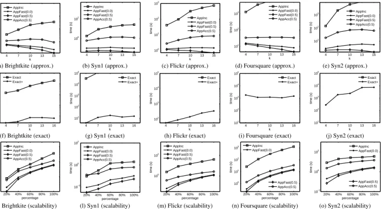
1. Effect ofkfor approximation algorithms.Figures 12(a)-(e) report the results. We skip the results on Gowalla, due to the space limitation. We can see thatAppFastruns consistently faster thanAppIncandAppAcc. For example, for the largest dataset Foursquare,AppFast(0.0)is at least two orders of magnitude faster than AppInc, although they return the same SACs.
AppFast(0.0)is 2 to 5 times faster thanAppAcc(0.5). This is becauseAppFasthas a lower time complexity. In addition, the running time ofAppFastdecreases as the value ofkincreases. This is becauseO(q, δ)becomes larger askincreases, and finding a largerO(q, δ)tends to need less binary search.