Detecting Differential Item and Step Functioning with Rating Scale and Partial Credit Trees

Detecting Differential Item and Step Functioning

with Rating Scale and Partial Credit Trees

Technical Report Number 152, 2014 Department of Statistics

University of Munich

with Rating Scale and Partial Credit Trees

Ludwig-Maximilians-Universit¨at M¨unchen Achim Zeileis Universit¨at Innsbruck Carolin Strobl Universit¨at Z¨urich Abstract

Several statistical procedures have been suggested for detecting differential item func-tioning (DIF) and differential step funcfunc-tioning (DSF) in polytomous items. However, standard procedures are designed for the comparison of pre-specified reference and focal groups, such as males and females.

Here, we propose a framework for the detection of DIF and DSF in polytomous items under the rating scale and partial credit model, that employs a model-based recursive partitioning algorithm. In contrast to existing procedures, with this approach no pre-specification of reference and focal groups is necessary, because they are detected in a data-driven way. The resulting groups are characterized by (combinations of) covariates and thus directly interpretable.

The statistical background and construction of the new procedures are introduced along with an instructive example. Four simulation studies illustrate and compare their statistical properties to the well-established likelihood ratio test (LRT). While both the LRT and the new procedures respect a given significance level, the new procedures are in most cases equally (simple DIF groups) or more powerful (complex DIF groups) and can also detect DSF. The sensitivity to model misspecification is investigated. An application example with empirical data illustrates the practical use.

A software implementation of the new procedures is freely available in the R system for statistical computing.

Keywords: partial credit model, rating scale model, differential item functioning, differential step function, measurement invariance, model-based recursive partitioning.

1. Introduction

A major concern in educational and psychological testing is the stability of measurement properties of a test or questionnaire between different groups of subjects, also known as measurement invariance. Violations of this property at the item level are known as item bias or differential item functioning (DIF). To assess if DIF is present, a variety of procedures have been proposed (for reviews see, e.g., Holland and Wainer 1993).

Nearly all of these procedures (e.g., the likelihood ratio test, Andersen 1973; Gustafsson 1980, the Mantel-Haenszel test, Holland and Thayer 1988, or logistic regression procedures,

Swaminathan and Rogers 2000and extensions and related procedures thereof, e.g.,Swanson, Clauser, Case, Nungester, and Featherman 2002; Van den Noortgate and De Boeck 2005) require a pre-specification of (usually) two groups which are then analyzed for the existence

of DIF. In practice, these groups are often formed by splitting the sample based on a few standard covariates such as gender or age. For numeric covariates like age, the median is often (relatively arbitrarily) used as split point (see, e.g., Sauer, Walach, Kohls, and Strobl 2013;Klooster, Taal, Siemons, Oostveen, Harmsen, Tugwell, Rader, Lyddiatt, and Laar 2013). An advantage of this approach is that the usage of observed covariates as splitting variables automatically provides some guidance for the interpretation of detected DIF. An obvious disadvantage is that DIF can only be denied for groups explicitly compared by the researcher, leaving the possibility that a later found group difference is only an artifact due to unnoticed DIF.

Based on a statistical algorithm called model-based recursive partitioning (Zeileis, Hothorn, and Hornik 2008), Strobl, Kopf, and Zeileis (2013) proposed an alternative DIF detection procedure for dichotomous items, that avoids a pre-specification of the groups being analyzed for DIF. Given a number of covariates, their procedure identifies groups with DIF in any item parameter of the dichotomous Rasch model by a recursive, data-driven test of all possible groups formed by (combinations of) covariates. Strobl et al. (2013) illustrated this for a variety of complex but realistic group patterns: e.g., DIF that is present only between females over a certain age and all other subjects (i.e., an interaction of two covariates age and gender), non-monotone patterns and groups formed by non-median splits in continuous covariates such as age (e.g., when both young and old participants are affected). As their procedure forms a closed testing procedure, it does not lead to an inflation of the type I error rate. Consequently, this alternative approach provides a more thorough DIF analysis while still maintaining the interpretability of the results.

Besides dichotomous items, polytomous items are often used as an alternative to allow for a more detailed response. As for dichotomous items, various DIF detection procedures exist for polytomous items (for reviews see, e.g., Potenza and Dorans 1995; Penfield and Lam 2000). Most of these procedures again require a pre-specification of groups and are therefore susceptible to the same problem as described above. As the model-based recursive partitioning algorithm is not restricted to the dichotomous Rasch model, an application of this algorithm to polytomous item response theory (IRT) models can provide a similarly thorough DIF detection procedure for polytomous items as was provided byStroblet al.(2013) for dichotomous items. Therefore, the aim of this paper is to develop and illustrate two extensions of the approach presented byStrobl et al.(2013) to DIF detection in polytomous items.

The extension of the model-based recursive partitioning algorithm to a polytomous IRT model not only provides a DIF detection procedure that identifies DIF groups in a data-driven way, it also – depending on the underlying IRT model – provides a procedure that is sensitive to measurement invariance at the individual score level, a phenomenon termed differential step functioning (DSF,Penfield 2007). The rationale is the following: As the model-based recursive partitioning algorithm considers instabilities in every parameter of a statistical model, and the parameters in polytomous IRT models most often describe some form of a transition between score levels, a procedure which is sensitive to DIF and DSF is the consequence. In addition, this sensitivity is independent of the sign of the effects and therefore not prone to a cancellation of diverging DSF effects within an item as some other existing procedures are, e.g., the polytomous SIBTEST procedure (Chang, Mazzeo, and Roussos 1996) or the polytomous DFIT approach (Flowers, Oshima, and Raju 1999). According to the classification ofPenfield, Alvarez, and Lee (2009), a global DIF statistic is provided, but opposed to other global DIF statistics, the graphical representation of the results can provide some information about the

precise score levels showing DSF and are thus responsible for item level DIF. In sum, the application of the model-based recursive partitioning algorithm to a polytomous IRT model provides a thorough DIF analysis procedure that is sensitive to both, DIF and DSF. (To facilitate readability, the term DIF always includes DSF in the following and the term DSF is only used to explicitly denote differential step functioning.)

In this paper, we present the extension of the model-based recursive partitioning algorithm to two well known polytomous IRT models, the rating scale model and the partial credit model and thus present two new DIF detection procedures for polytomous items. After an introduction of the rating scale and partial credit model in the next section, a more detailed introduction of the model-based recursive partitioning algorithm, along with an artificial in-structive example, follows in Section 3. Section4contains the results of a series of simulation studies to support and illustrate the statistical properties of the proposed procedures together with performance comparisons to the well-established likelihood ratio test. Finally, an appli-cation example with empirical data is presented in Section 5. A software implementation of the proposed procedures is freely available in the add-on package psychotree(Zeileis, Strobl, Wickelmaier, and Kopf 2014) for theRsystem for statistical computing (RCore Team 2013).

2. Rating scale and partial credit model

The rating scale model (RSM, Andrich 1978) and the partial credit model (PCM, Masters 1982) are two widely applied polytomous Rasch models. The RSM,

P(Xij =xij|θi, βj,τ) = exp xij X k=0 (θi−(βj +τk)) p X `=0 exp ` X k=0 (θi−(βj+τk)) (1)

describes the probability that subject i with person parameter θi scores in one of the p

categories of item j. Items are modeled by means of two parameters in the RSM: an item location parameter βj, describing the overall location of item j on the latent scale and a set

of threshold parameters τ = (τ1, . . . , τk, . . . , τp)>, describing the distance between the overall

location βj, and the transition points from one category to the next category (see Figure 1

for an illustration).

As becomes clear from Equation 1, the number and values of the threshold parameters τk

is constant over all items j, which restricts the RSM to a set of items with the same num-ber of categories and also assumes equal distances between the intersections of the category characteristic curves of two adjacent categories over all items.

The PCM, P(Xij =xij|θi,δj) = exp xij X k=0 (θi−δjk) pj X `=0 exp ` X k=0 (θi−δjk) (2)

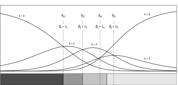
Index Probability k=0 k=1 _k=2 k=3 k=4 δj1 δj2 δj4 δj3 βj+ τ1 βj+ τ2 βj+ τ4 βj+ τ3 Latent trait θ

Figure 1: Category characteristic curves (above) and effect plot (below) with regions of most probable category responses (i.e., the modes) of an item with five categories. In addition, the locations of RSM and PCM parameters are depicted.

relaxes these assumptions by allowing a variable number of categories and spacing of the intersections of the category characteristic curves per item. While θi is still the person

pa-rameter of subject i, each item is now described by a set of threshold parameters δj =

(δj1, . . . , δjk, . . . , , δjpj)>, which mark the intersections between the probability curves of two

adjacent categories, i.e., the point where the probability of scoring in category k−1 is the same as scoring in category k. This is illustrated in Figure1.

In the upper part of Figure 1, the category characteristic curves of an artificial item with five categories are shown. For given item and person parameters, these curves describe the probability of responding in a category as predicted under the RSM or the PCM. The positions of the RSM and the PCM threshold parameters are depicted, showing their location at the intersection between the category characteristic curves of two adjacent categories.

An alternative illustration, that was already used byVan der Linden and Hambleton(1997) in the context of IRT and has been called “effect displays” byFox and Hong (2009), is shown in the lower part of Figure1. In this illustration, only the regions of the most probable category responses (i.e., the modes) of an item over the range of the latent trait are shown. As inFox and Hong (2009), this type of illustration will be called “effect plot” from here on and will be later used as means of illustrating the results of the newly proposed DIF procedures.

For ordered threshold parameters, i.e., increasing in their value with the response categories, the locations of the borders of the regions in the effect plot directly correspond to the values of the threshold parameters. Otherwise they are given by the mean (Wilson and Masters 1993) between two adjacent unordered threshold parameters. A discussion of the meaning of unordered threshold parameters can be found in Andrich (2013). In our implementation, we inform the user about the existence of unordered threshold parameters within an item by depicting their locations with dashed lines (see Figure 1). From the point of view of the proposed procedures, unordered threshold parameters do not pose a problem because only

parameter differences between groups and not their order is considered.

In the next section, the model-based recursive partitioning algorithm and its extension to the RSM and the PCM is described in more detail.

3. Detecting polytomous DIF with recursive partitioning

Similar to the procedure proposed by Strobl et al. (2013), the two new DIF detection pro-cedures for polytomous items proposed in the following are based on a statistical algorithm called model-based recursive partitioning (Zeileis et al. 2008). Model-based recursive par-titioning is a semi-parametric approach that employs statistical tests for structural change adopted from econometrics. The aim is to detect differences in the parameters of a statistical model between groups of subjects defined by (combinations of) covariates.

Model-based recursive partitioning is related to – but by means of modern statistical tech-niques avoids the earlier weaknesses of – the method of classification and regression trees (CART, Breiman, Friedman, Olshen, and Stone 1984; see Strobl, Malley, and Tutz 2009

for a thorough introduction), where the covariate space is recursively partitioned to identify groups of subjects with different values of a categorical or numeric response variable. As an advancement of this approach, in model-based recursive partitioning it is the parameters of a parametric model – rather than the values of a single response variable – that vary between groups. Such parameters could be, e.g., intercept and slope parameters in a linear regression model or, as it is the case here, the parameters of a RSM or a PCM that may vary between groups of subjects and thus indicate the presence of DIF.

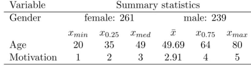
This principle is now first illustrated by means of an artificial instructive example with the PCM, before the technical details are addressed for both, the RSM and the PCM, in the next sections. The data for the instructive example are the responses of 500 hypothetical subjects to 8 items with 3 categories per item simulated under the PCM. These data can be considered, e.g., as responses to an attainment test. In addition to the responses, the data set includes three covariates: gender, age, and a motivation score. The summary statistics of these covariates are reported in Table 1.

Table 1: Summary statistics of the covariates of the instructive example (artificial data).

Variable Summary statistics

Gender female: 261 male: 239

xmin x0.25 xmed x¯ x0.75 xmax

Age 20 35 49 49.69 64 80

Motivation 1 2 3 2.91 4 5

The data of the instructive example were simulated with DIF between males and females in item 2 and 3: All threshold parameters of these items were higher for males than for females, i.e., it was simulated to be more difficult for males to get a higher score on these items. In addition, the threshold parameters of item 6 and 7 have been reversed for males but not for females to illustrate how unordered threshold parameters are indicated in the graphical output of our procedure. Between females up to the age of 40 and females over the age of 40, DSF was simulated in item 4 and 5, i.e., only the first threshold parameter of these items

Gender p < 0.001 1 male female Node 2 (n = 226) I1 I2 I3 I4 I5 I6 I7 I8 −4 −2 0 2 4 Latent tr ait Age p < 0.001 3 ≤40 >40 Node 4 (n = 93) I1 I2 I3 I4 I5 I6 I7 I8 −4 −2 0 2 4 Latent tr ait Node 5 (n = 157) I1 I2 I3 I4 I5 I6 I7 I8 −4 −2 0 2 4 Latent tr ait

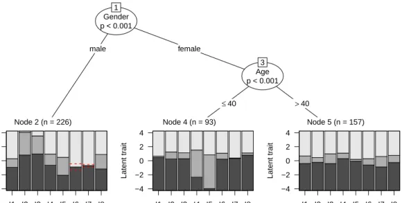
Figure 2: Partial credit tree for the instructive example (artificial data for illustration pur-poses), exhibiting DIF between males and females in item 2 and 3 and reversed thresholds in item 6 and 7. In addition, DSF is present in the first threshold parameter of item 4 and 5 between females up to the age of 40 and females over the age of 40 years. In the terminal nodes, effect plots are depicted for each item with the estimated threshold parameters of the PCM in the corresponding node.

was different between these two groups such that younger females were simulated to have a lower threshold between the first and second category (see Figure 2 for an illustration of the results). No DIF was simulated with respect to the covariate motivation.

In order to detect DIF with the proposed procedure, the item responses are assessed with respect to possible group differences related to the three covariates gender, age, and motiva-tion, as described in detail below. The resulting model, that is partitioned with respect to a combination of the covariates gender and age, is presented in Figure 2 and will be termed a partial credit tree (or a rating scale tree if the RSM is used for partitioning) from here on. In each of the terminal nodes of the tree, an effect plot like that in Figure 1 is shown for each item. As in Figure 1, these plots show regions of most probable category responses (i.e., the modes) over the range of the latent trait as defined by the estimated threshold parameters of the PCM in the corresponding node.

Overall, the mere fact that there is more than one terminal node in Figure 2 means that the null hypothesis of one joint PCM for the entire sample (i.e., measurement invariance) must be rejected. In this sense, the proposed procedure is a global test for DIF as well as an overall model test for the PCM (or the RSM for rating scale trees). But in contrast to most other global tests for DIF, the results can be visualized as a tree (see Figure 2) and hence convey much more information concerning the detected DIF than just a simple test statistic. The visualization shows the identified subgroups, their characterization by given covariates and aids in the identification of the specific items that are affected by DIF or DSF. All these information can help to generate hypotheses about possible underlying sources of these effects

and guide the decision how to proceed.

With respect to the results of the instructive example (Figure2), we find that the simulated DIF pattern has been correctly recovered: Different threshold parameters have been detected for males and females, and within the group of females for those up to the age of 40 and those over the age of 40. The estimated threshold parameters of item 2 and 3 have higher values for males (node 2) than for females (node 4 and 5). In addition, reversed threshold parameters for males in item 6 and 7 are indicated by dashed lines. Within the group of females, the first threshold parameters of item 4 and 5 are much lower for females up to the age of 40 (node 4) than for females above the age of 40 (node 5) thus indicating DSF in this item.

It is important to note, that all that was passed over to the algorithm to detect DIF, were the three covariates age, gender and the motivation score. Neither the specific subgroups nor the cutpoint within the numeric covariate age was pre-specified. Both had to be detected by means of the available data. Especially the data-driven detection of the cutpoint within the numeric covariate age is in contrast to the widely employed approach of arbitrarily splitting a numeric variable at the median (which for the subgroups of females would have been at the value 47 and thus too high). This common practice would not only have concealed the actual age at which the parameter change occurs but may even result in not detecting significant DIF in a numeric variable at all, as was shown by Strobl et al. (2013) for the Rasch tree approach and as is further illustrated in the simulation studies below for the procedures newly proposed here. In addition to the successful detection of DIF, i.e., a shift in one or more threshold parameters, the fact that only single threshold parameters in two items differ between females up to the age of 40 and above the age of 40 (i.e., DSF) was also correctly discovered by the partial credit tree. Moreover, the variable motivation was not selected for splitting (i.e., no DIF or DSF was detected with respect to motivation), which also correctly replicates the simulated pattern.

The data-driven identification of DIF groups (which may be formed by complex interactions of covariates or non-trivial cutpoints in numeric covariates) is a key feature of the model-based recursive partitioning approach employed here, that makes it very flexible for detecting groups with DIF or DSF and distinguishes it from other (parametric) DIF detection procedures, where DIF can only be detected in those groups explicitly compared.

Technically, the following consecutive steps are used to infer the structure of a partial credit tree like that depicted in Figure 2from the data:

1. Estimate the model parameters jointly for all subjects in the current sample, starting with the full sample.

2. Assess the stability of the item or threshold parameters with respect to each available covariate.

3. If there is significant instability, split the sample along the covariate with the strongest instability and in the cutpoint leading to the highest improvement of model fit.

4. Repeat steps 1–3 recursively in the resulting subsamples until there are no more signif-icant instabilities (or the subsample becomes too small).

These four steps are now explained in more detail and the extension of the approach ofStrobl

3.1. Estimating the model parameters

Since the person raw-scoresri=Pmj=1xij form sufficient statistics for the person parameters

in Rasch models (Andersen 1977), a conditional maximum likelihood approach can be used. In this approach, the conditional likelihoods given in Equation3for the RSM and in Equation4

for the PCM are maximized by means of iterative procedures to estimate the item- and threshold-parameters. Lc(β,τ|r1, . . . , rn) = n Y i=1 Lc(β,τ|ri) = n Y i=1 exp (−Pmj=1(xij·βj+ Pxij k=0τk)) γri(β,τ) (3) Lc(δ|r1, . . . , rn) = n Y i=1 Lc(δ|ri) = n Y i=1 exp (₋Pm_j=1Pxij k=0δjk) γri(δ) (4)

In Equation3as well as in Equation4,γri are the elementary symmetric functions of orderri

(cf., e.g., Fischer and Molenaar 1995). To fix the origin of the scale, for both equations some constraint has to be applied, leaving m+p₋2 free parameters in the RSM and Pm_j=1pj−1

free parameters in the PCM.

3.2. Testing for parameter instability

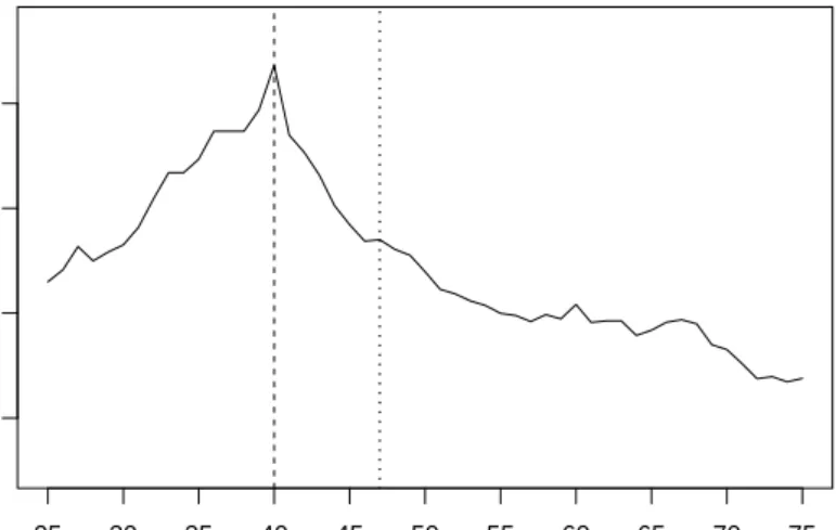
In order to test whether the model parameters vary between groups of subjects defined by covariates, we use the approach of structural change tests from econometrics. The rationale of these tests is the following: The model parameters are first estimated jointly for the entire sample. Then the individual deviations from this joint model are ordered with respect to a covariate, such as age. If there is systematic DIF or DSF with respect to groups formed by the covariate, the ordering will exhibit a systematic change in the individual deviations. If, on the other hand, no DIF or DSF is present, the values will merely fluctuate randomly. This rationale is explained in detail in Zeileiset al.(2008) and Strobl et al. (2011;2013) but is shortly illustrated in Figure 3: In this example, the individual contributions of all subjects to the score function, that is used for the estimation of a parameter, are ordered with respect to the variable age. By definition, the score contributions are zero on average. However, when the score contributions are ordered with respect to the variable age, it becomes obvious that they do not fluctuate randomly around the mean zero – which would be the case under the null hypothesis that one joint parameter estimate is appropriate for the entire sample – but there is a systematic change at the age of 40. This systematic change indicates that, instead of one joint parameter estimate for the entire sample, different parameter estimates should be permitted for subjects up to the age of 40 and above the age of 40.

Zeileis and Hornik (2007) and Zeileis et al. (2008) have shown that it is possible to derive statistical tests for parameter change from the path of the cumulated score contributions, that converges to a Brownian bridge under the null hypothesis of parameter stability. As the result of these parameter instability tests, test statistics and associated (Bonferroni-adjusted, see also Section 3.4) pvalues are provided for each candidate variable.

An advantage of this approach is that the model does not have to be re-estimated for all splits in all covariates, because the individual score contributions remain the same and only their ordering needs to be adjusted for evaluating the different covariates.

Age

Individual score contr

ib utions 25 30 35 40 45 50 55 60 65 70 75 −0.25 0 0.25

Figure 3: Structural change in the variable age (artificial data for illustration purposes). The individual score contributions are ordered with respect to the variable age. The dashed lines indicate deviations from the overall mean zero, which are positive before the structural change and negative afterwards.

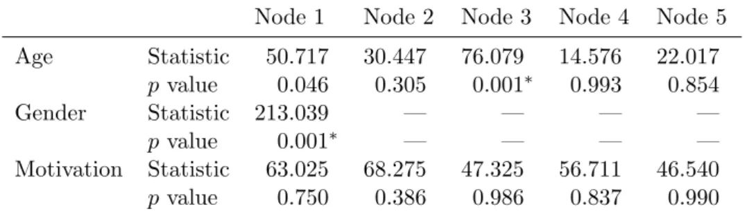
Table 2: Summary of the parameter instability test statistics and corresponding Bonferroni-adjusted pvalues for the instructive example. Those variables whosepvalues are highlighted with an asterisk are selected for splitting in the respective node.

Node 1 Node 2 Node 3 Node 4 Node 5

Age Statistic 50.717 30.447 76.079 14.576 22.017 p value 0.046 0.305 0.001∗ _{0.993 0.854} Gender Statistic 213.039 — — — — p value 0.001∗ — — — — Motivation Statistic 63.025 68.275 47.325 56.711 46.540 p value 0.750 0.386 0.986 0.837 0.990

For the RSM and the PCM, the individual score functions can easily be computed from the conditional likelihoods given in Equation 3 and Equation4and are provided in AppendixA. Based on the individual score functions, the above outlined structural change tests can easily be applied. The results of these tests for the instructive example are shown in Table 2. In the first node, the variable with the smallest p value – in this case gender – is selected for splitting (cf. Table2and Figure2). In each daughter node the splitting continues recursively: Here, the variable age is selected for splitting in the third node, whereas no further splits are found significant in the second and all the following nodes.

−1400 −1380 −1360 −1340 Age Log−Lik elihood 25 30 35 40 45 50 55 60 65 70 75

Figure 4: Partitioned log-likelihood for the second split in the covariate age. The dashed line indicates the location of the optimal cutpoint (at the value 40) while the dotted line indicates the location of the median (at the value 47) for the subgroup of females.

Note that the variable gender is no longer available for splitting after the first node because it offers only one possible cutpoint (that has already been used for the first split). As opposed to gender, the second splitting variable age offers as many possible cutpoints as it has distinct values. In this case, it is an important advantage of the model-based recursive partitioning method that the exact cutpoint does not need to be pre-specified, but is determined in a data-driven way as described in detail in Section 3.3.

Splitting continues until allpvalues exceeded the significance level (commonly 5%), indicating that there is no more significant parameter instability, or until the number of observations in a subsample falls below a given threshold (see also Section 3.4).

3.3. Selecting the cutpoints

After a covariate has been selected for splitting, the optimal cutpoint is determined by max-imizing the partitioned log-likelihood (i.e., the sum of the log-likelihoods for two separate models: one for the observations to the left and up to the cutpoint, and one for the obser-vations to the right of the cutpoint) over all candidate cutpoints within the range of this variable.

For the first split in the instructive example, the selection of the cutpoint is trivial – since the binary variable gender only allows for a single split between the subgroups of females and males. In the second split, however, all possible cutpoints in the variable age for the female subsample are considered and the associated partitioned log-likelihood is displayed in Figure 4. The value 40 is selected as the optimal cutpoint, because it shows the highest value of the partitioned log-likelihood, i.e., the strongest differences in the threshold parameters

exist between females up to the age of 40 and over the age of 40.

Note that other potential cutpoints close to this value also show a high value of the partitioned log-likelihood, so that in different random samples from the same underlying population not always the same value for the optimal cutpoint may be detected. However, from Figure 4it is obvious that the median (dotted line), that is often used for pre-specifying the reference and focal groups from a numeric predictor variable, may be far off the maximum of the partitioned log-likelihood indicating the strongest parameter change. As opposed to that, the data-driven approach suggested here cannot only reliably detect the parameter instability in the variable age, but it can also identify at what age the strongest parameter change occurs (as was also systematically illustrated by the simulation results of Stroblet al. 2013).

While this approach can be applied to numeric and ordered covariates, for unordered cate-gorical covariates the categories can be split into any two groups. From all these candidate binary partitions, again the one that maximizes the partitioned log-likelihood is chosen. Selecting the optimal cutpoint by maximizing the partitioned (log-)likelihood corresponds directly to using the maximum likelihood ratio (LR) statistic of the joint vs. the partitioned model. Hence fortesting whether there is significant DIF or DSF in a covariate, the computa-tionally cheap LM test is used, while for estimating where the strongest DIF or DSF occurs, the computationally costly LR test is used.

From a statistical point of view, this two-step approach – where the variable selection is made independently from the cutpoint selection – has two important advantages: Not only does it considerably reduce the computational burden, but at the same time it also prevents an artifact termed variable selection bias (cf., e.g.,Shih 2004;Hothorn, Hornik, and Zeileis 2006;

Strobl, Boulesteix, and Augustin 2007), that was inherent in earlier recursive partitioning algorithms.

3.4. Stopping criteria

For creating a rating scale or partial credit tree, the four basic steps outlined above – (1) es-timating the parameters of a joint model, (2) testing for parameter instability, (3) selecting the splitting variable and cutpoint and (4) splitting the sample accordingly – are repeated recursively until a stopping criterion is reached.

Two kinds of stopping criteria are currently implemented: The first is to stop splitting if there is no (more) significant instability with respect to any of the covariates. Thus, the significance level – usually set to 5% – serves as stopping criterion. As second stopping criterion, a minimum sample size per node can be specified. This minimal node-size should be chosen such as to provide a sufficient basis for parameter estimation in each subsample, and should thus be adjusted to the number of model parameters. In our examples, we have chosen a significance level of 5% and a minimal node-size of 20 for rating scale trees and 30 for partial credit trees.

Finally, one should keep in mind that when a large number of covariates is available in a data set, and all those covariates are to be tested for DIF, multiple testing becomes an issue – as with any statistical test for DIF. To account for the fact that multiple testing might lead to an increased false-positive rate when the number of available covariates is large, a Bonferroni adjustment for the p value splitting criterion is applied internally.

for overfitting: In classical algorithms (such as CART; Breiman et al. 1984) a pruning step (i.e. cutting back branches at the bottom of the tree that do not add to the prediction accuracy in cross-validation) is necessary to make sure that any splits detected for the learning data do not only reflect random variation but also generalize to other samples from the same data generating process. As opposed to these classical algorithms, the model-based recursive partitioning approach employed here is already based on statistical inference tests (rather than merely descriptive statistics) and uses their p values (together with several precautions against multiple testing) for stopping before overfitting occurs (see also Hothornet al.2006). Therefore, pruning is not necessary in this approach.

Moreover, it is important to note that the model-based recursive partitioning algorithm is not affected by an inflation of chance due to its recursive nature. Indeed, several statistical tests are successively conducted in a rating scale or partial credit tree – but each test is conducted only if the previous test yielded a significant result. In this sense, the recursive approach forms a closed testing procedure, which does not lead to an inflation of chance as is well known from the literature on multiple comparisons (Marcus, Peritz, and Gabriel 1976;

Hochberg and Tamhane 1987). For the rating scale and partial credit trees this means that the postulated significance level holds for the entire tree, not only for each individual split. This ensures that DIF or DSF are not erroneously detected as an artifact of the recursive nature of the algorithm.

In the following, the statistical properties of rating scale and partial credit trees are analyzed by means of a series of simulation studies.

4. Simulation studies

Four simulation studies were conducted to illustrate and assess the statistical properties of rating scale and partial credit trees. In addition, the likelihood ratio test (LRT, Andersen 1973;Gustafsson 1980) was included as a basis of comparison. The LRT was chosen because it is a DIF detection procedure which is parametric, i.e., based on an underlying IRT model and global, i.e., does not only test a single item for DIF (for details see, e.g.,Penfield and Lam 2000;

Potenza and Dorans 1995). In this sense, the LRT is comparable to the procedures proposed here. In addition, simulation studies have shown that the LRT has comparable or better statistical properties than several other existing DIF detection procedures for polytomous items (Bolt 2002;Woods 2011).

All simulation studies were conducted in the statistical software R (RCore Team 2013). To fit rating scale and partial credit trees we used our own freely available package psychotree (Zeileiset al. 2014). The statistical software R, as well as the above mentioned package are freely available under the General Public License (GPL) from the Comprehensive RArchive Network (CRAN).

After a description of the criterion variables and the experimental settings used in all simula-tion studies, the four simulasimula-tion studies are explained in more detail in the following secsimula-tions.

4.1. Criterion variables and experimental settings

The following two criterion variables have been used to measure the performance of the procedures in the simulation studies:

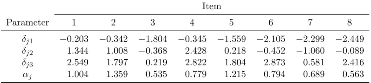
Table 3: Item threshold and discrimination parameters of a 1992 NAEP calibration with the graded response model (Samejima 1969) byJohnson and Carlson (1994).

Item Parameter 1 2 3 4 5 6 7 8 δj1 −0.203 −0.342 −1.804 −0.345 −1.559 −2.105 −2.299 −2.449 δj2 1.344 1.008 −0.368 2.428 0.218 −0.452 −1.060 −0.089 δj3 2.549 1.797 0.219 2.822 1.804 2.873 0.581 2.416 αj 1.004 1.359 0.535 0.779 1.215 0.794 0.689 0.563

Percentage of significant test results: Depending on the presence of DIF or DSF, this

criterion variable reflects the type I error (no DIF or DSF present) or power (DIF or DSF present) of the underlying procedure. Consequently, this criterion variable should not exceed the given significance level in settings without DIF or DSF and should be preferably high in settings with DIF or DSF. For rating scale and partial credit trees the percentage of splits in the first node was recorded as the percentage of significant results, i.e., if any instability in the model parameters was detected.

Root mean squared error (RMSE): The RMSE, computed as the root mean squared

difference between the true (simulated) and the estimated parameter values of the item with DIF or DSF, is a measure of parameter recovery. Smaller values indicate a better recovery of the true (simulated) parameter and group structure. The RMSE is only displayed when group recovery is of interest.

In addition to the experimental factors varied within the four simulation studies, the following settings have been used in all simulation studies:

Significance level: α= 0.05 was used as the significance level.

Number of replications: 10,000 replications were conducted for each experimental scenario

to ensure an appropriate precision of the estimates of the criterion variables.

Number of observation: n= 1000 was used as overall sample size.

Number of items, categories and item parameters: To make the simulation studies

re-alistic as well as comparable to already published simulation studies, we used a set of item parameters estimated with the graded response model (GRM, Samejima 1969) in a calibration of the 1992 NAEP (Johnson and Carlson 1994) which have also been used in simulation studies by Changet al. (1996);Camilli and Congdon (1999) andPenfield and Algina (2006). This set consists of discrimination parametersαj and threshold

pa-rametersδjk of eight polytomous items with four categories each (see Table3). We used

parameter estimates from the (more general) GRM to be able to investigate the effects of model misspecification (see simulation study III for details). In all other simulation studies, the discrimination parameters are ignored and the threshold parameters are used in the RSM and the PCM as described below.

Person parameters: Person ability parameters were drawn from a normal distribution

τk) for the RSM and µ= Pm1 j=1pj Pm j=1 Ppj k=1δjk for the PCM.

Procedures: Four procedures were compared in all simulation studies: rating scale trees

(“TREE-RSM”), partial credit trees (“TREE-PCM”), LRT with the RSM as the under-lying model RSM”) and LRT with the PCM as the underunder-lying model (“LRT-PCM”).

Model used for generating the data: The RSM, the PCM and the GRM have been used

as IRT models to generate the data. For the RSM, the mean of all item threshold parameters δjk of an item j from Table 3has been used as item location parameter βj

and the mean of all differences between item threshold parameters δ_j(k−1) and δjk has

been used as threshold parameterτk. For the PCM, the item threshold parametersδjk

as given in Table3have been used while ignoring the item discrimination parametersαj.

For the GRM (only used in simulation study III), both the item threshold parameters

δjk as well as the item discrimination parametersαj as given in Table3have been used.

4.2. Simulation study I: Basic functioning

The first simulation study illustrates the basic functioning of the TREE procedures. In addition, the performance of these procedures is compared to the well-established LRT either under the null hypothesis of no DIF or the alternative of DIF being present.

For simplicity only the percentage of significant test results is reported as criterion variable in this first simulation study.

The computation times of both types of procedures in this first simulation study can be found in AppendixB.

Design of simulation study I

In the following, the experimental factors that have been varied are described in more detail:

DIF pattern: DIF pattern “none” represents the null hypothesis scenario, where there are

no differences between the item threshold parameters of the reference and focal groups. DIF pattern “constant-0.5” on the other hand represents the alternative of DIF being present. In this scenario, all item threshold parameters (or the item location parameter in the RSM) of item 5 of the focal group have been shifted by a constant value of= 0.5.

Covariate pattern: This experimental factor represents the covariate pattern that specified

the reference and focal groups.

In the setting “binary”, a binary covariate was sampled from a binomial distribution with equal class probabilities. Under the DIF setting, DIF was then simulated between the two groups corresponding directly to the two categories of this binary covariate. In the setting “numeric”, a numeric covariate was sampled from a discrete uniform distribution over the values 1 to 100. Under the DIF setting, DIF was then simulated between the two groups specified by splitting the observations at the median of the numeric covariate.

In the settings “both-binary” and “both-numeric”, both covariates were present in the data but only the binary or the numeric covariate was used to specify reference and

focal groups in settings with DIF while the other covariate was present as a nuisance variable.

For the LRT procedures, the variable defining reference and focal groups and for numeric covariates also a cutpoint has to be specified a priori. In settings with a single covariate, this covariate was used to define reference and focal groups. When both covariates were present, the LRT was computed for each covariate. To have comparable results between the TREE and the LRT procedures in these settings, the resulting p-values of the LRT procedures have been Bonferroni-adjusted, like thep-values of the TREE procedures when there is more than one covariate available for splitting (cf. Section 3.4). In addition, for numeric covariates, the “correct” cutpoint, i.e., the median, was pre-specified for the LRT procedues. This is different

in simulation study II, where the influence of misspecified cutpoints is analyzed.

For the TREE procedures it is important to note that in contrast to the LRT procedures the split variable (in the “both” settings) as well as the cutpoint for numeric covariates have to be located in a data-driven way as additional tasks. While the first task is done by selecting the covariate with the smallest (Bonferroni-adjusted) p value, the second task is done by a search over all possible binary partitions (cf. Section 3.3). For correct specifications of the split variable and the cutpoint in the LRT procedures, these tasks can be a disadvantage for TREE procedures. For DIF groups formed by unknown or non-standard covariate patterns, however, this additional flexibility is an advantage as can be seen in simulation study II. A major concern often formulated here is that the multiple tests or the search over all binary partitions conducted by the TREE procedures may lead to a type I error inflation. This is not the case as can be seen in the following results.

In this simulation study an IRT model corresponding to the DIF procedure was used to generate the data, i.e., for TREE-RSM and LRT-RSM the RSM was used as IRT model to generate the data, while for TREE-PCM and LRT-PCM the PCM was used as IRT model to generate the data. This is different in simulation study III where the effect of model misspecification is analyzed. In addition, no ability differences between reference and focal groups have been simulated here, but will be also investigated in simulation study III.

Results of simulation study I

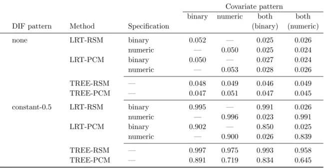
As can be seen in the upper six rows of Table 4, all procedures roughly respect the given significance level of 0.05 under the null hypothesis of no DIF. This is especially true for the TREE procedures when a numeric or both covariates are present. Hence neither the binary search over all possible cutpoints in numeric covariates nor the variable selection task when multiple covariates are present cause an type I error inflation. Note again that the results for the LRT procedures in these settings are listed seperately for the binary and the numeric covariate and are Bonferroni-adjusted like the results of the TREE procedures incorperating the search over both covariates.

The performance under the alternative, i.e., constant DIF of = 0.5 in one item, is reported in the lower six rows of Table 4. Whereas for binary covariates the power of the TREE procedures is comparable or only slightly lower than the power of the corresponding LRT procedures, the power of the trees is notably lower in settings with a numeric covariate. This is caused by the underlying maximum LM test, where for moderate sample sizes the discrete empirical fluctuation process always fluctuates slightly less than its continuous asymptotic counterpart, the Brownian bridge (cf. Strobl et al. 2013). Note however that this apparent

Table 4: Results of simulation study I – Percentage of significant test results in settings without (“none”) and with (“constant-0.5”) DIF for various covariate patterns.

Covariate pattern

binary numeric both both DIF pattern Method Specification (binary) (numeric)

none LRT-RSM binary 0.052 — 0.025 0.026 numeric — 0.050 0.025 0.024 LRT-PCM binary 0.050 — 0.027 0.024 numeric — 0.053 0.028 0.026 TREE-RSM — 0.048 0.049 0.046 0.049 TREE-PCM — 0.047 0.051 0.047 0.045 constant-0.5 LRT-RSM binary 0.995 — 0.991 0.026 numeric — 0.996 0.023 0.991 LRT-PCM binary 0.902 — 0.850 0.025 numeric — 0.900 0.026 0.839 TREE-RSM — 0.997 0.975 0.993 0.958 TREE-PCM — 0.891 0.719 0.834 0.645

disadvantage of the TREE procedures in comparison to the LRT procedures only affects the most often unrealistic situation where exactly the correct cutpoint in a numeric covariate is known a priori and provided to the LRT. More realistic settings where the true cutpoint is unknown or misspecified are presented in the next simulation study.

When both covariates are present, the TREE procedures again perform very well despite the additional variable selection task. The power is only slightly lower than in the corresponding setting with only one covariate being present. The power of the LRT procedures on the other hand is completely dependent on the correct specification of the covariate defining reference and focal groups. If the “wrong” covariate is used, the percentage of significant test results actually represents the type I error and therefore is near the Bonferroni-adjusted significance level of 0.025. With a correctly specified covariate, the power is slightly lower compared to the corresponding setting with only one covariate due to the Bonferroni adjustment in these settings.

In addition, an effect of the underlying item response model can be seen from Table 4. In all settings with the PCM, the power is lower than in corresponding settings with the RSM. Hence the more restricted item response model leads to a higher power for both types of DIF detection procedures – if the IRT model used to generate the data is correctly specified (Note that in this simulation study the same model that was used for generating the data is also used for the analysis. See simulation study III for the effects of the misspecification of the data generating model).

4.3. Simulation study II: More complex reference and focal groups

In simulation study I, the covariate patterns specifying reference and focal groups have been very simple. This is often not the case in empirical data, where reference and focal groups can result from more complex covariate patterns (see Section 5 for an example). Simulation

study II therefore illustrates how the TREE procedures as well as the LRT procedures per-form when DIF is present in reference and focal groups specified by more complex covariate patterns.

To see how well the true (simulated) parameter values are recovered in such more complex groups, the RMSE is reported in addition to the percentage of significant test results as criterion variable.

Design of simulation study II

In the following, the more complex covariate patterns used in this simulation study are de-scribed in detail. Whereas the categorical covariate has been sampled from a discrete uniform distribution with levels 1–4, the binary and the numeric covariate have again been sampled from the same distributions as in simulation study I.

Categorical: In this setting, DIF was simulated between two groups specified by a

combi-nation of the levels of a categorical covariate (levels 1 and 3 for the reference group and levels 2 and 4 for the focal group). This pattern corresponds to a situation with a categorical covariate like, e.g., “hobby”, where DIF is present only for subjects with certain hobbies, e.g., chess and strategy games vs. football and dancing.

Numeric-80: In this setting, DIF was simulated between two groups specified by a single

numeric covariate but with a cutpoint at the constant value of 80. This pattern corre-sponds to a situation with a numeric covariate like age, where DIF is present only for older subjects.

U-shaped: In this setting, DIF was simulated between two groups specified by values of the

numeric covariate up to the value 20 and from the value 80 vs. values between 20 and 80. This patterns corresponds to a situation with a numeric covariate like age, where DIF is present for young and old subjects as opposed to middle-aged subjects.

Interaction-median: In this setting, DIF was simulated between two groups specified by

those observations with a value of 1 in the binary covariate and a value of the nu-meric covariate above the median vs. all other observations. This pattern corresponds to a situation where DIF is present only for a subgroup of subjects resulting from a combination of two covariates, e.g., females above the median age.

Interaction-80: This setting is identical to the setting “interaction-median” execpt that a

constant value of 80 instead of the median was used as cutpoint for the numeric covariate. This pattern corresponds again to a situation where DIF is present only for a subgroup of subjects resulting from a combination of two covariates and a non-trivial cutpoint, e.g., females above the age of 80.

In the interaction settings, the LRT procedures again require the specification of a covariate that defines reference and focal groups. As before, we computed the LRT with Bonferroni-adjusted p-values for each possible covariate. In the setting with a categorical covariate, the distinct levels of this covariate have been used to specify the focal groups, i.e., one group consisting of all subjects (reference group) was compared to four subgroups resulting from the four levels of the categorical covariate (focal groups). We have choosen this approach because

Table 5: Results of simulation study II – Power of the four DIF detection procedures for five more complex covariate patterns.

Covariate pattern

categorical numeric-80 u-shaped interaction interaction

Method Specification (median) (80)

LRT-RSM binary — — — 0.392 0.061 numeric — 0.328 0.051 0.398 0.062 categorical 0.961 — — — — LRT-PCM binary — — — 0.166 0.040 numeric — 0.177 0.052 0.170 0.039 categorical 0.669 — — — — TREE-RSM — 0.954 0.801 0.687 0.518 0.187 TREE-PCM — 0.632 0.419 0.276 0.228 0.089

in practice, it is usually unknown if any levels of a categorical covariate can be combined and therefore all possible subgroups are used as focal groups. For numeric covariates, we again used the median as the cutpoint for the LRT procedures because this is often done in practice. For the TREE procedures, all these specifications are again not necessary because the groups are detected in a data-driven way.

Like in simulation study I (see there for details), an IRT model corresponding to the DIF procedure was used to generate the data and no ability differences between reference and focal groups have been simulated. In addition, constant DIF of = 0.5 was present in all settings of simulation study II.

Results of simulation study II

As can be seen in Table 5, the power observed in this simulation study is generally lower than the power observed in simulation study I. This is a consequence of the more complex covariate patterns that form reference and focal groups in this simulation study compared to the simple covariate patterns used in simulation study I.

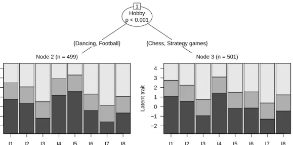
In the setting with a categorical covariate (see Figure5for an examplary tree of this setting), the power of the TREE procedures is comparable or only slightly lower than the power of the LRT procedures. (As described below, the main difference in this setting between the two types of DIF procedures can be seen in the RMSE). In all remaining covariate pattern settings the TREE procedures are more powerful than the corresponding LRT procedures. In the “numeric-80” and “u-shaped” settings, this is a consequence of the fact that – as often in practice – the median was used as the naive cutpoint for defining reference and focal groups in the LRT procedures. In the interaction settings, this is a consequence from considering only a single covariate in the LRT procedures while the true (simulated) groups result from a combination of two covariates. Both situations pose no problems for the TREE procedures. Because of the data-driven detection of reference and focal groups for these procedures, non-standard cutpoints as well as more complex groups can be detected and no a priori knowledge is necessary.

Like in simulation study I, an effect of the underlying item response model can be found in simulation study II. Procedures with the RSM are again more powerful than the corresponding

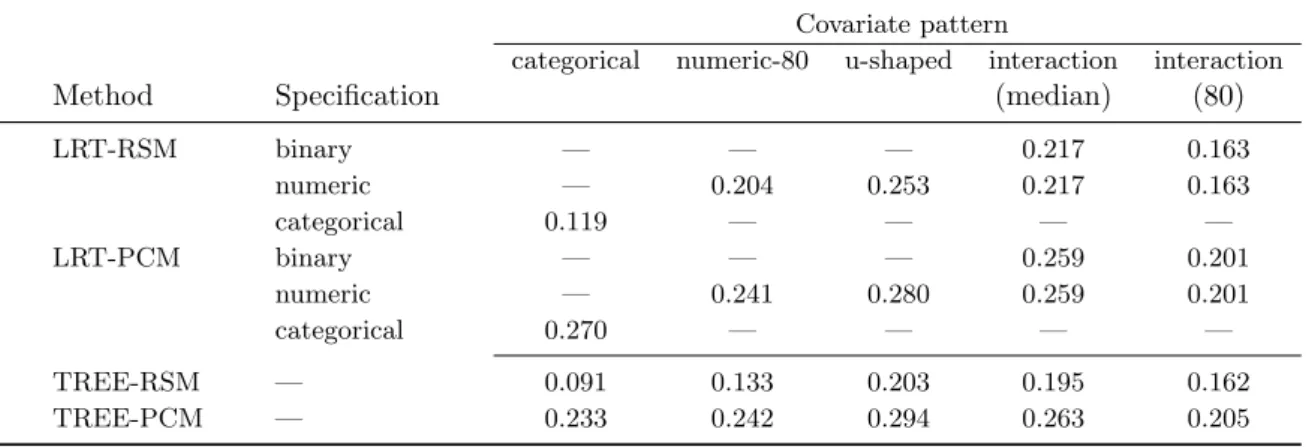
Table 6: Results of simulation study II – RMSE of the four DIF detection procedures for five more complex covariate patterns.

Covariate pattern

categorical numeric-80 u-shaped interaction interaction

Method Specification (median) (80)

LRT-RSM binary — — — 0.217 0.163 numeric — 0.204 0.253 0.217 0.163 categorical 0.119 — — — — LRT-PCM binary — — — 0.259 0.201 numeric — 0.241 0.280 0.259 0.201 categorical 0.270 — — — — TREE-RSM — 0.091 0.133 0.203 0.195 0.162 TREE-PCM — 0.233 0.242 0.294 0.263 0.205

procedures with the PCM.

In addition to the power, the RMSE is reported in Table 6. Here lower values indicate a better recovery of the true (simulated) parameters and group structure. In the setting with a categorical covariate it is interesting to see that even though the power of the TREE proce-dures was comparable or slightly lower than the power of the corresponding LRT proceproce-dures (see Table 5), the former are better able to recover the true (simulated) parameters as is indicated by the lower RMSE. This is due to the (wrongly) pre-specified reference and focal groups in the LRT procedures. These have been – as often in practice – naively specified by the distinct levels of the categorical covariate and hence the item threshold parameters have been estimated separately for subjects with the same level of the categorical covariate. As the true groups have been simulated by a combination of several levels of the categorical covariate, the pre-specification used in the LRT procedures is actually a overspecification and estimation precicion is lost by estimating the same item threshold parameters separately. The more flexible data-driven detection of the TREE procedures provides an advantage in such a situation. These procedures are able to estimate the item threshold parameters in (detected) subgroups based on several levels of the categorical covariate and therefore a more precise estimation is possible. The result of the TREE procedures in one iteration of this setting of the simulationy study is examplarily illustrated in Figure 5. In the settings with a numeric covariate pattern or an interaction covariate pattern, the RMSE of the TREE procedures is lower then the RMSE of the LRT procedures only with the RSM as underlying IRT model. With the PCM as underlying IRT model, the RMSE is comparable or slightly higher for the TREE procedure compared to the LRT procedure. This is due to the higher number of pa-rameters to be estimated under the PCM compared to the RSM which require a high sample size for the more flexible TREE procedures to be estimated precisely.

Concerning the two interaction settings, it is interesting to note that the RMSE of both classes of procedures is much lower with the cutpoint at the value of 80 compared to the median, even though DIF in this setting is harder to detect, i.e., the power is lower. This is due to the different ratio of reference and focal group in these settings. In the setting with the median as cutpoint, this ratio is 75% vs. 25%, i.e., 75% of the subjects belong to the reference group and 25% belong to the focal group. In the setting with the value of 80 as cutpoint, this ratio is 90% vs. 10%, i.e., 90% of the subjects belong to the reference group and only 10% belong

Hobby p < 0.001

1

{Dancing, Football} {Chess, Strategy games}

Node 2 (n = 499) I1 I2 I3 I4 I5 I6 I7 I8 −2 −1 0 1 2 3 4 Latent tr ait Node 3 (n = 501) I1 I2 I3 I4 I5 I6 I7 I8 −2 −1 0 1 2 3 4 Latent tr ait

Figure 5: Example result of the TREE procedures in the setting with a categorical covariate pattern in simulation study II. Based on simulated parameter differences (i.e., DIF) in item 5, some levels (and hence subjects inhibiting these levels) of the categorical covariate (which for illustration purposes has been named “Hobby” here) have been combined.

to the focal group. When the focal group is proportionally smaller, it is harder for the two classes of procedures to detect it as a seperate group, i.e., the power is lower. However, as the subjects of each group share the same item or threshold parameters, the overall RMSE for estimating the item or threshold parameters is lower, because a larger number of item parameters can be more reliably estimated from a larger sample.

4.4. Simulation study III: Model misspecification and ability differences

As parametric DIF detection procedures, the TREE procedures as well as the LRT proce-dures assume that the observed data follow a specific item response model. This assumption often has been mentioned as disadvantage of this class of procedures (see e.g., Potenza and Dorans 1995). But to our knowledge, so far onlyBolt(2002) has examined the consequences of violations of this assumption, i.e., model misspecifiation (or model misfit as it is named in Bolt 2002), systematically. Although Bolt (2002) only used 100 replications per setting, a type I error inflation was found for the LRT with the GRM as underlying IRT model and the generalized partial credit model (Muraki 1992) or the two-parameter sequential response model (Mellenbergh 1995) as data generating IRT models which was more pronounced with increasing sample size. Interestingly, this type I error inflation was only seen when there was an additional ability difference between reference and focal groups, indicating that the earlier found robustness of the LRT procedure to ability differences (Kim and Cohen 1998;

Ankenmann, Witt, and Dunbar 1999) may only be valid when there is no additional model misspecification. The following simulation study examines the consequences of model mis-specification and ability differences on the type I error rates of the TREE procedures as well

as the LRT procedures and tries to replicate the above cited findings for these procedures. For simplicity only the percentage of significant test results, i.e., the type I error in this simulation study, is reported as criterion variable.

Design of simulation study III

In the following, the experimental factors that have been varied are described in more detail:

Ability differences: In settings with no ability differences, person ability parameters of

reference and focal groups were drawn from a normal distribution N(µ,1) with µ as the mean of all item or threshold parameters , i.e., µ = _m1_·pPm_j=1Pp_k=1(βj +τk) for

the RSM andµ= Pm1 j=1pj

Pm j=1

Ppj

k=1δjk for the PCM. This is identical to the previous

simulation studies.

In addition, ability differences of ∆∈ {−0.5,−0.25,0.25,0.5} have been simulated. For these settings, the person ability parameters of the reference group were drawn from a normal distribution N(µ− ∆₂,1) whereas the person ability parameters of the focal group were drawn from a normal distribution N(µ+∆₂,1).

Model misspecification: Model misspecification was simulated by using a different IRT

model to generate the data than the underlying model of the DIF detection procedure: For the TREE-PCM procedure and the LRT-PCM procedure the RSM or the GRM were used as data generating IRT models. For the TREE-RSM procedure and the LRT-RSM procedure the PCM and the GRM were used as data generating IRT models (see Section4.1for a more detailed description of the IRT models to generate the data). In addition, the “correct” IRT model to generate the data have also been included which means all three IRT models to generate the data have been used for all four different DIF detection procedures.

In all settings of this simulation study a binary covariate (again sampled from a binomial distribution with equal class probabilities) was used to specify reference and focal groups. There were no differences in the item or threshold parameters (i.e., no DIF) between these groups, because the emphasis of this simulation study was on the type I error.

Results of simulation study III

The type I error rates of the four DIF detection procedures (columns) conditional on ability differences between reference and focal groups (x-axis) and the IRT model to generate the data (rows) are illustrated in Figure 6. Settings with model misspecification are marked by the capital letter “M”. The dashed line indicates the given significance level of 0.05.

It can be seen that no type I error inflation is present in settings without model misspecification for any procedure. This is also the case in settings where the IRT model to generate the data is nested in the assumed model of the DIF detection procedures, i.e., in settings with the RSM as IRT model to generate the data and a DIF detection procedure with the PCM as the underlying model.

As can be seen from Figure 6, the tree-based DIF detection procedures even get slightly conservative with increasing ability differences in these settings (as was already noted by

LRT−RSM LRT−PCM TREE−RSM TREE−PCM M M M M M M M M M M M M M M M M M M M M M M M M M M M M M M M M M M M M M M M M 0.0 0.2 0.4 0.6 0.8 0.0 0.2 0.4 0.6 0.8 0.0 0.2 0.4 0.6 0.8 RSM PCM GRM −0.5 −0.25 0 0.25 0.5 −0.5 −0.25 0 0.25 0.5 −0.5 −0.25 0 0.25 0.5 −0.5 −0.25 0 0.25 0.5 Ability differences T ype I error

Figure 6: Results of simulation study III – Type I error of the four DIF detection procedures (columns) conditional on ability differences between reference and focal groups (x-axis) and the IRT model to generate the data (rows). Settings with model misspecification are marked by the capital letter “M”. The dashed line indicates the given significance level of α= 0.05.

not shown) indicate that it occurs for all likelihood-based DIF tests: the score test employed in the TREE procedures, the classical Wald test (Glas and Verhelst 1995) as well as the LRT (Andersen 1973;Gustafsson 1980) – for which, however, the effect occurs only for larger ability differences than those that were used in this simulation study, so that the effect for the LRT is not visible in the results presented here. Note again, however, that the tests behave conservatively rather than inflating the significance level, as one might fear for test-intensive methods like the TREE procedures.

When model misspecification is present, a type I error inflation occurs for both types of procedures only if there are additional ability differences. Thus for LRT procedures as well as the TREE procedures neither model misspecification nor ability differences alone lead to a type I error inflation. In addition, for both experimental factors (model misspecification and ability differences) the type I error inflation is more pronounced with increased model misspecification or ability differences. These effects are independent of the direction of the ability differences.

Overall, the results extend the robustness of the LRT procedure to model misspecification

procedure to ability differences (Kim and Cohen 1998; Ankenmann et al. 1999) to settings where no additional violations of the underlying assumptions of these procedures are present.

4.5. Simulation study IV: Differential step functioning

In polytomous items not only the properties of a whole item but also the properties of single response categories can vary between groups of subjects, i.e., DSF. While simulation study I and II assessed the performance of the methods when DIF (i.e., a constant shift of all score categories) is present, simulation study IV illustrates the performance of these procedures with various patterns of DSF.

For simplicity only the percentage of significant test results, i.e., the power in this simulation study, is reported as criterion variable.

Design of simulation study IV

Due to the item parametrization in the RSM (for all items the same distance between two categories is assumed) it is not possible to simulate DSF in a single item with this model. Therefore, the PCM was used in all settings as IRT model to generate the data. This auto-matically implies a situation of model misspecification for the TREE-RSM procedure and the LRT-RSM procedure. But as no ability differences were simulated in this simulation study, no type I error inflation occurs as was shown in simulations study III.

The DSF patterns used in our simulation study were taken from the literature and have already been used in simulation studies by Wang and Su (2004); Su and Wang (2005) and

Penfield (2010). In the following, they are described in more detail:

Single-level: In this setting, the first item threshold parameter of item 5 of the focal group

was shifted by = 0.5. This corresponds to DSF in a single category.

Convergent: In this setting, the first and third item threshold parameter of item 5 of the

focal group were shifted by= 0.5 and= 0.25 respectively.

Divergent: In this setting, the first and third item threshold parameter of item 5 of the focal

group were shifted by= 0.5 and=−0.25 respectively.

Balanced: In this setting, the first and third item threshold parameter of item 5 of the focal

group were shifted by = 0.5 and=−0.5 respectively. This leads to a cancellation of DSF in item 5, i.e., the overall region of this item on the latent trait gets smaller but the mean of the item threshold parameters remains the same.

In all settings of this simulation study a binary covariate (again sampled from a binomial distribution with equal class probabilities) was used to specify reference and focal groups. No ability differences between reference and focal groups have been simulated.

Results of simulation study IV

The results of simulation study IV are reported in Table7. All four DIF detection procedures are sensitive to DSF, even in a single category. In contrast to other existing DIF detection procedures for polytomous items, e.g., the polytomous SIBTEST procedure (Chang et al.

Table 7: Results of simulation study IV – Power of the four DIF detection procedures for four DSF patterns together with the overall absolute DSF size in each setting.

Method

DSF pattern Overall abs. DSF size LRT-RSM LRT-PCM TREE-RSM TREE-PCM

single-level 0.50 0.148 0.206 0.130 0.193

convergent 0.75 0.261 0.251 0.254 0.248

divergent 0.75 0.084 0.248 0.085 0.234

balanced 1.00 0.093 0.439 0.099 0.429

1996) or the polytomous DFIT approach (Flowerset al. 1999), this is also the case when the DSF effects are balanced. (We did not include the aforementioned polytomous DIF detection procedures in this simulation study because these are item-wise in contrast to the global DIF detection procedures compared here.) The power of the TREE procedures is comparable or only slightly lower than the power of the corresponding LRT procedure. Because of the comparable power of the two types of procedures (TREE and LRT), we only distinguish between RSM procedures and PCM procedures in the following.

Concerning these two types of procedures it should first be noted that in contrast to the results of simulation study I and II with constant DIF, it now becomes obvious that procedures with the RSM as the underlying model are not generally more powerful than procedures with the PCM as the underlying model. The results in Table 7 show that the power of the PCM procedures is roughly a function of the overall absolute DSF effect size. For the RSM procedures on the other hand, diverging or balanced DSF effects lead to a rather strong decrease in power although these DSF patterns have the highest overall absolute DSF size. As explained in the following, these effects can be attributed to the different item parametrization in the two models (RSM and PCM) underlying these procedures.

In the PCM, where each transition between two categories is modeled by a single item thresh-old parameter δjk, DSF in single response categories can – independent of its sign – directly

be captured by a single model parameter. In the RSM however, there is no single parameter for each individual transition but one location parameter that models the overall position of an item and several threshold parametersτk, that model the transitions between two adjacent

categories that are, however, assumed to be the same for all items.

Therefore, shifts in one or more threshold parameters of a single item like in the “single-level” or “divergent” settings cannot directly be captured in the RSM and consequently a lower power is observed for the class of RSM procedures compared to the class of PCM procedures. Furthermore, since for divergent or balanced DSF the overall position of the item does not (balanced DSF) or only slightly (divergent DSF) change, it can be assumed that these types of DSF have no effect on the item location parameterβj in the RSM. Hence only the threshold

parameters remain to capture such shifts. But since these are computed over all items, shifts in categories of a single item as simulated here are most likely covered by the stable distances in all other items and therefore the power to detect such shifts is low for procedures with the RSM as underlying model.

5. Application: DIF in the Freiburg mindfulness inventory

The Freiburg mindfulness inventory (FMI, Walach, Buchheld, Buttenm¨uller, Kleinknecht, and Schmidt 2006) is a self-report questionnaire to measure the concept of mindfulness, “an ancient Buddhist practice [. . . which. . . ] means paying attention in a particular way: on purpose, in the present moment, and nonjudgementally” (Kabat-Zinn 2005, p. 3–4). In the following, we focus on the subscale “presence” of a short version of the FMI. Each of the five items has six response categories (1 – completely disagree, . . . , 6 – completely agree) and is reported in Table8.

Table 8: Items of the subscale “presence” of a short version of the Freiburg mindfulness inventory (FMI, Walachet al. 2006).

Item Label

1 I am open to the experience of the present moment.

2 I sense my body, whether eating, cooking, cleaning or talking.

3 When I notice an absence of mind, I gently return to the experience of the here and now. 4 I pay attention to what’s behind my actions.

5 I feel connected to my experience in the here and now.

To detect DIF in the subscale “presence”, Saueret al. (2013) analyzed the responses of 1059 subjects with the LRT procedure and the RSM as underlying IRT model. Amongst others, the following four covariates have been used to define reference and focal groups: Age (with the median as cutpoint), gender, mode of data collection (online/offline) and previous experience with mindfulness meditation (yes/no). The summary statistics of these covariates based on a slightly reduced data set (n= 1032, removed subjects below the age of 16 or who scored in category 1 or 5 at all items) used in the following are reported in Table 9.

Table 9: Summary statistics of the four considered covariates.

Covariate Summary statistics

Gender female: 694 male: 338

Experience yes: 420 no: 612

Mode online: 952 offline: 80

xmin x0.25 xmed x¯ x0.75 xmax

Age 16 26 33 35.10 44 77

According to the results reported by Sauer et al. (2013), the null hypothesis of no DIF has to be rejected for the covariates “previous experience with mindfulness meditation”, χ2_{(8) =}

78.71, p < 0.001, and “mode of data collection”, χ2(7) = 19.71, p = 0.006 (Item 5 was excluded due to a null category), but not for the covariates age, χ2(8) = 11.59, p = 0.171, and gender, χ2_{(8) = 12.89, p = 0.116. Besides slightly different numerical results, the}

conclusions remain the same in our modified data set.

As it is common in DIF analysis with the LRT procedure, Saueret al. (2013) only compared groups defined by a single covariate. This leaves DIF in groups resulting from interactions