İSTANBUL TECHNICAL UNIVERSITY INSTITUTE OF SCIENCE AND TECHNOLOGY
Ph.D. Thesis by Yusuf YASLAN
Department : Computer Engineering Programme : Computer Engineering
DECEMBER 2010
SUPERVISED AND SEMI-SUPERVISED LEARNING USING INFORMATIVE FEATURE SUBSPACES
İSTANBUL TECHNICAL UNIVERSITY INSTITUTE OF SCIENCE AND TECHNOLOGY
Ph.D. Thesis by Yusuf YASLAN
(504042506)
Date of submission : 19 October 2010 Date of defence examination : 02 December 2010
Supervisor (Chairman) : Assoc. Prof. Dr. Zehra ÇATALTEPE (ITU)
Members of the Examining Committee : Prof. Dr. Muhittin GÖKMEN (ITU) Assoc. Prof. Dr. Berrin YANIKOĞLU (SU)
Assoc. Prof. Dr. Tunga GÜNGÖR (BU) Assist. Prof. Dr. Şule GÜNDÜZ – ÖĞÜDÜCÜ (ITU)
DECEMBER 2010
SUPERVISED AND SEMI-SUPERVISED LEARNING USING INFORMATIVE FEATURE SUBSPACES
ARALIK 2010
İSTANBUL TEKNİK ÜNİVERSİTESİ FEN BİLİMLERİ ENSTİTÜSÜ
DOKTORA TEZİ Yusuf YASLAN
(504042506)
Tezin Enstitüye Verildiği Tarih : 19 Ekim 2010 Tezin Savunulduğu Tarih : 02 Aralık 2010
Tez Danışmanı : Doç. Dr. Zehra ÇATALTEPE (İTÜ) Diğer Jüri Üyeleri : Prof. Dr. Muhittin GÖKMEN (İTÜ) Doç. Dr. Berrin YANIKOĞLU (SÜ) Doç. Dr. Tunga GÜNGÖR (BÜ) Yrd. Doç. Dr. Şule GÜNDÜZ – ÖĞÜDÜCÜ (İTÜ)
BİLGİ İÇEREN ÖZNİTELİK ALT UZAYLARI İLE EĞİTMENLİ VE YARI EĞİTMENLİ ÖĞRENME
FOREWORD
First of all I would like to thank to my supervisor Dr. Zehra Çataltepe for her support and effort during my academic research. I believe that without her enthusiasm on research, this thesis would never be finished. Thanks also go to her for proofreading the thesis book that significantly improved the quality of the thesis.
Next I would like to thank to the progress committee members Dr. Berrin Yanıkoğlu and Dr. Şule Gündüz-Öğüdücü for their valuable time and comments in the periodical meetings.
During the last couple years Kenan Kule has been my roommate. He didn't hesitate to help me whenever I needed. I would like to thank him for his help. I also thank to members and research assistants of the Computer Engineering Department at Istanbul Technical University: Berk Canberk, Tolga Ovatman, Burak Kantarcı, Melike Erol-Kantarcı, Çağatay Talay, Nagehan İlhan, Figen Şentürk, Gülnur Selda Kuruoğlu, Aycan Atak and Mustafa Ersen. Besides during my assistantship at the Department, Tacettin Ayar and Dr. A. Cüneyd Tantuğ were always with me with their friendships. I'd like to also thank to them.
Last I would like to thank my mother, my father and my brother. I could have never achieved my goals without their valuable support.
December 2010 Yusuf Yaslan
TABLE OF CONTENTS
Page
FOREWORD ... v
TABLE OF CONTENTS ... vii
ABBREVIATIONS ... ix
LIST OF TABLES ... xi
LIST OF FIGURES ... xiii
LIST OF SYMBOLS ... xvii
SUMMARY ... xix
ÖZET ... xxi
1. INTRODUCTION ... 1
1.1 Contributions of the Thesis ... 4
2. CLASSIFIER ENSEMBLES AND DIVERSITY ... 7
2.1 Classifier Ensembles ... 7
2.1.1 Bagging ... 9
2.1.2 Boosting ... 9
2.1.3 Mixture of experts ... 10
2.1.4 Stacked generalization ... 11
2.1.5 Input decimated ensembles ... 11
2.1.6 Classifier combination methods in classifier ensembles ... 11
2.1.6.1 Combinations of abstract level outputs ... 12
2.1.6.2 Combinations of ranked lists ... 13
2.1.6.1 Combinations of continuous outputs ... 13
2.2 Measures of Diversity for Classifier Ensembles ... 13
2.2.1 Pairwise measures ... 14
2.2.2 Non-pairwise measures ... 15
2.3 Information Theoretic Analysis of the Classifier Ensembles ... 16
3. SUPERVISED LEARNING USING INFORMATIVE FEATURE SUBSPACES ... 21
3.1 Related Work ... 21
3.2 Random Subspaces (RAS) ... 23
3.3 Relevant Random Subspaces (Rel-RAS) ... 24
3.4 Minimum Redundancy and Maximum Relevance Random Subspaces (mRMR-RAS) ... 26
3.5 Accuracy Analysis of the Subspace Selection Algorithms ... 27
3.6 Experimental Results ... 29
3.6.1 Real data results ... 30
3.6.2 Robustness to redundant features ... 36
3.6.3 Synthetic data results ... 37
3.6.4 Classifier diversity and information theoretic analysis of the algorithms in supervised learning ...39
4. SEMI-SUPERVISED LEARNING USING INFORMATIVE FEATURE
SUBSPACES ... 47
4.1 Related Work ... 49
4.2 Co-training ... 52
4.3 Random Subspaces for Co-training (RASCO) ... 53
4.4 Relevant Random Subspace Method for Co-training (Rel-RASCO) ... 54
4.5 Minimum Redundancy and Maximum Relevance Random Subspace Method for Co-training (mRMR-RASCO) ... 54
4.6 Experimental Results ... 56
4.6.1 Real data results ... 56
4.6.2 Robustness to redundant features ... 64
4.6.3 Synthetic data results ... 65
4.6.4 Classifier diversity and information theoretic analysis of the algorithms in supervised learning ...66
4.7 Discussion ... 70
4.7.1 The effect of unlabeled data ... 71
5. CONCLUSION AND FUTURE WORK ... 73
REFERENCES ... 77
APPENDICES ... 85
ABBREVIATIONS
RAS : Random Subspaces
Rel-RAS : Relevant Random Subspaces
mRMR-RAS : minimum Redundancy Maximum Relevance Random
Subspaces
RASCO : Random Subspaces for Co-training
Rel-RASCO : Relevant Random Subspaces for Co-training
mRMR-RASCO : minimum Redundancy Maximum Relevance Random
Subspaces for Co-training
KNN : K - Nearest Neighbour
LDC : Linear Discriminant Classifier
SVM : Support Vector Machines
RM : Recursively More
KW : Kohavi - Wolpert
LOD : Low Order Diversity
ITS : Information Theoretic Score ITA : Information Theoretic Accuracy ITD : Information Theoretic Diversity MID : Mutual Information Distance MIQ :Mutual Information Quotient
LIST OF TABLES
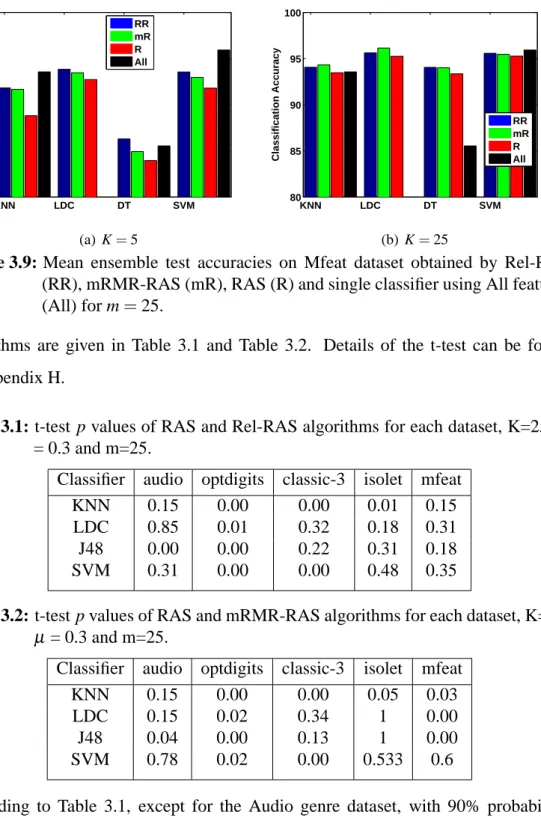
Page Table 2.1: The 2x2 relationship between classifiers with probabilitiess ... 14 Table 3.1: t-test p values of RAS and Rel-RAS algorithms for each dataset K=25,
μ = 0.3 and m=25. ... 35 Table 3.2: t-test p values of RAS and mRMR-RAS algorithms for each dataset
K=25, μ = 0.3 and m=25 . ... 35 Table 4.1: t-test p values of RASCO and Rel-RASCO at the beginning and at the
end of the algorithms for each dataset K=25, m=25 . ... 63 Table 4.2: t-test p values of RASCO and mRMR-RASCO at the beginning and at
the end of the algorithms for each dataset K=25, m=25 . ... 63 Table C.1 : Real Datasets. ... 89
LIST OF FIGURES
Page
Figure 1.1 : Scenarios of different input/output feature availability (Extended from [1]). Rows correspond to objects/instances. Wide boxes are feature matrices, narrow boxes correspond to labels. Available data are represented in blue, missing data that can be queried by a learning algorithm are represented in purple color...2 Figure 1.2 : a) Unsupervised and b) supervised learning algorithms illustration
on two dimensional feature space...3 Figure 2.1 : General framework of classifier ensembles [2]....8 Figure 3.1 : Mean ensemble and individual test accuracies on Audio Genre
dataset obtained by mRMR-RAS, Rel-RAS, RAS and single classifier with respect toµ for K=5, m=25 and classifier = KNN....30 Figure 3.2 : Mean ensemble and individual test accuracies on Audio Genre
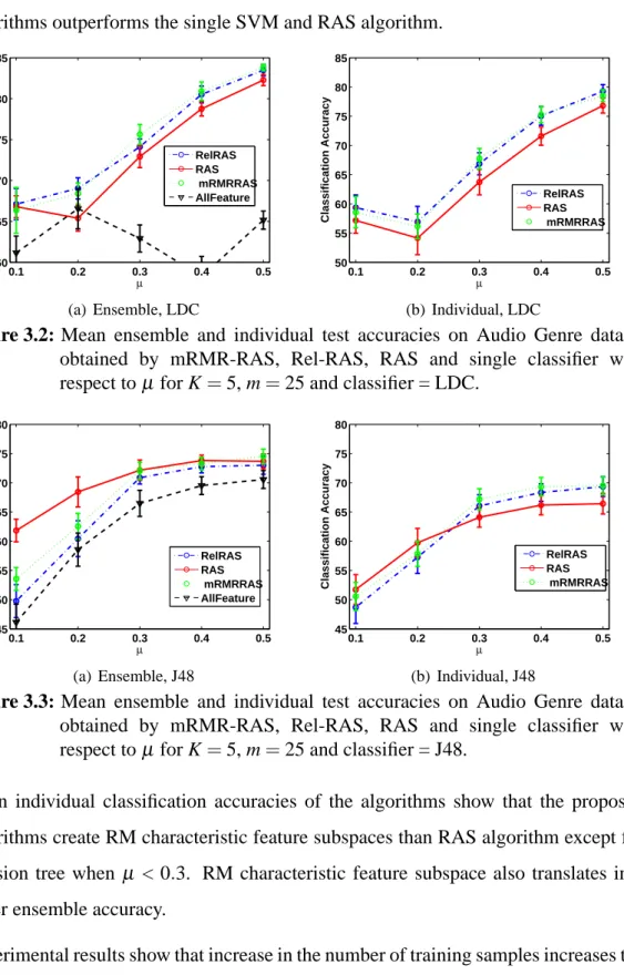
dataset obtained by mRMR-RAS, Rel-RAS, RAS and single classifier with respect toµ for K=5, m=25 and classifier = LDC....31 Figure 3.3 : Mean ensemble and individual test accuracies on Audio Genre
dataset obtained by mRMR-RAS, Rel-RAS, RAS and single classifier with respect toµ for K=5, m=25 and classifier = J48...31 Figure 3.4 : Mean ensemble and individual test accuracies on Audio Genre
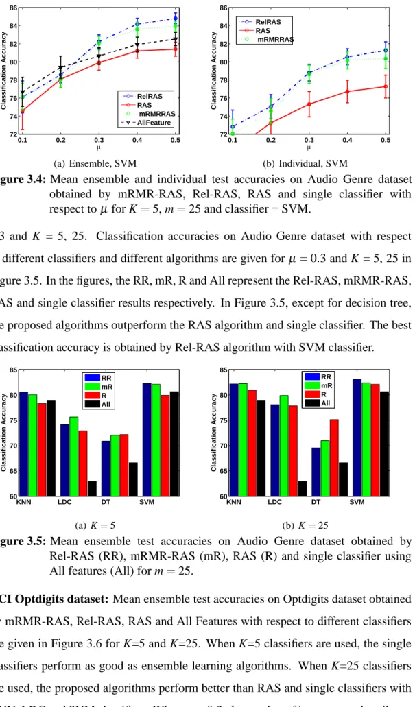
dataset obtained by mRMR-RAS, Rel-RAS, RAS and single classifier with respect toµ for K=5, m=25 and classifier = SVM...32 Figure 3.5 : Mean ensemble test accuracies on Audio Genre dataset obtained
by Rel-RAS (RR), mRMR-RAS (mR), RAS (R) and single classifier using All features (All) for m=25...32 Figure 3.6 : Mean ensemble test accuracies on Optdigits dataset obtained by
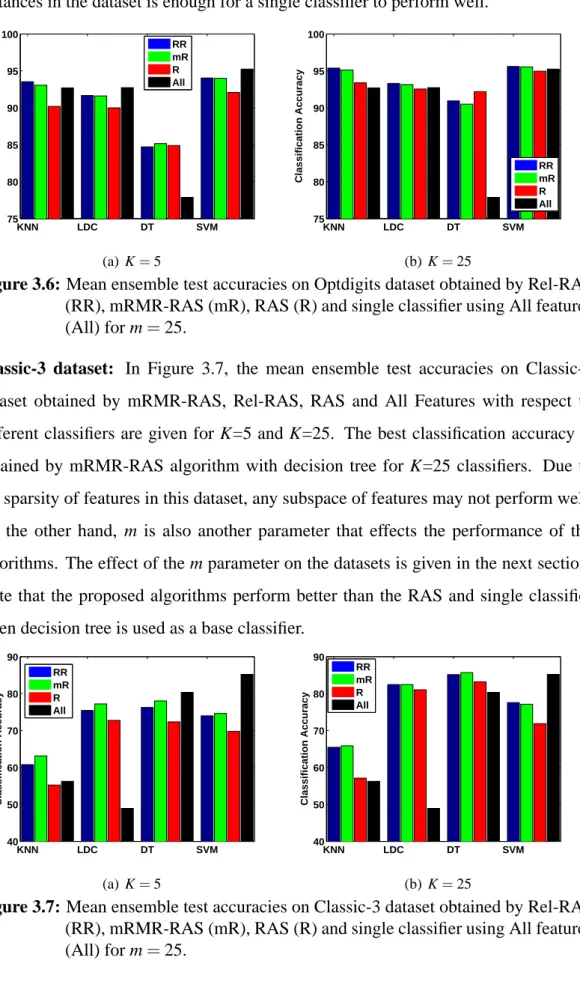
Rel-RAS (RR), mRMR-RAS (mR), RAS (R) and single classifier using All features (All) for m=25...33 Figure 3.7 : Mean ensemble test accuracies on Classic-3 dataset obtained by
Rel-RAS (RR), mRMR-RAS (mR), RAS (R) and single classifier using All features (All) for m=25...33 Figure 3.8 : Mean ensemble test accuracies on Isolated Letter Speech dataset
obtained by Rel-RAS (RR), mRMR-RAS (mR), RAS (R) and single classifier using All features (All) for m=25...34 Figure 3.9 : Mean ensemble test accuracies on Mfeat dataset obtained by
Rel-RAS (RR), mRMR-RAS (mR), RAS (R) and single classifier using All features (All) for m=25...35 Figure 3.10: a) Relevance, redundancy analysis and b) redundancy map of
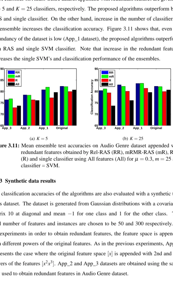
Figure 3.11: Mean ensemble test accuracies on Audio Genre dataset appended with redundant features obtained by Rel-RAS (RR), mRMR-RAS (mR), RAS (R) and single classifier using All features (All) for µ =0.3, m=25 and classifier = SVM...37 Figure 3.12: a) Relevance, redundancy analysis and b) redundancy map of
synthetic dataset appended with redundant features...38 Figure 3.13: Mean ensemble test accuracies on synthetic dataset appended
with redundant features obtained by Rel-RAS (RR), mRMR-RAS (mR), RAS (R) and single classifier using All features (All) for µ =0.3, m=25 and classifier = SVM...38 Figure 3.14: Classification accuracy versus diversity on Audio Genre dataset
obtained by mRMR-RAS, Rel-RAS and RAS for µ =0.3, K = 5,25 and m=25 a)KW-variance b) LOD c) ITS...40 Figure 3.15: Classification accuracy versus diversity on Optdigits dataset
obtained by mRMR-RAS, Rel-RAS and RAS for µ =0.3, K = 5,25 and m=25 a)KW-variance b) LOD c) ITS...41 Figure 3.16: Classification accuracy versus diversity on Classic-3 dataset
obtained by mRMR-RAS, Rel-RAS and RAS for µ =0.3, K = 5,25 and m=25 a)KW-variance b) LOD c) ITS...41 Figure 3.17: Classification accuracy versus diversity on Isolated dataset
obtained by mRMR-RAS, Rel-RAS and RAS for µ =0.3, K = 5,25 and m=25 a)KW-variance b) LOD c) ITS...42 Figure 3.18: Classification accuracy versus diversity on Mfeat dataset obtained
by mRMR-RAS, Rel-RAS and RAS for µ =0.3, K=5,25 and m=25 a)KW-variance b) LOD c) ITS...42 Figure 3.19: Classification accuracy versus m on Classic-3 dataset obtained by
Rel-RAS (RR), mRMR-RAS (mR), RAS (R) and single classifier using All features (All) forµ =0.3, K=25 and Classifier = SVM...44 Figure 4.1 : Mean ensemble and individual test accuracies on Audio Genre
dataset obtained by mRMR-RASCO, Rel-RASCO and RASCO with respect toµ for m=25, classifier = KNN...58 Figure 4.2 : Mean ensemble and individual test accuracies on Audio Genre
dataset obtained by mRMR-RASCO, Rel-RASCO and RASCO with respect to mu for m=25, classifier = LDC...59 Figure 4.3 : Mean ensemble and individual test accuracies on Audio Genre
dataset obtained by mRMR-RASCO, Rel-RASCO and RASCO with respect to mu for m=25, classifier = J48...59 Figure 4.4 : Mean ensemble and individual test accuracies on Audio Genre
dataset obtained by mRMR-RASCO, Rel-RASCO and RASCO with respect to mu for m=25, classifier = SVM...59 Figure 4.5 : Mean ensemble test accuracies on Audio Genre dataset, at
the beginning (-B) and end (-E) of Co-training, obtained by Rel-RASCO (RR), mRMR-RASCO (mR), RASCO (R) and single classifier using all features (All) for m=25...60 Figure 4.6 : Mean ensemble test accuracies on Optdigits dataset, at the
beginning (-B) and end (-E) of Co-training, obtained by Rel-RASCO (RR), mRMR-RASCO (mR), RASCO (R) and single classifier using all features (All) for m=25...61
Figure 4.7 : Mean ensemble test accuracies on Classic-3 dataset, at the beginning (-B) and end (-E) of Co-training, obtained by Rel-RASCO (RR), mRMR-RASCO (mR), RASCO (R) and single classifier using all features (All) for m=25...61 Figure 4.8 : Mean ensemble test accuracies on Isolated Letter Speech dataset,
at the beginning (-B) and end (-E) of Co-training, obtained by Rel-RASCO (RR), mRMR-RASCO (mR), RASCO (R) and single classifier using all features (All) for m=25...62 Figure 4.9 : Mean ensemble test accuracies on Mfeat dataset, at the beginning
(-B) and end (-E) of Co-training, obtained by Rel-RASCO (RR), mRMR-RASCO (mR), RASCO (R) and single classifier using all features (All) for m=25...62 Figure 4.10: Mean ensemble and individual classifier test accuracies on Audio
Genre dataset at the beginning (-B) and end (-E) of Co-training, obtained by Rel-RASCO (RR), mRMR-RASCO (mR), RASCO (R) and single classifier using all features (All), with respect to m for K=5 and classifier = SVM...64 Figure 4.11: Mean ensemble test accuracies on Audio Genre dataset appended
with redundant features, at the beginning (-B) and end (-E) of Co-training, obtained by Rel-RASCO (RR), mRMR-RASCO (mR), RASCO (R) and single classifier using all features (All), for µ =0.3, m=25 and classifier = SVM...65 Figure 4.12: Mean ensemble test accuracies on synthetic dataset appended
with redundant features, at the beginning (-B) and end (-E) of Co-training, obtained by Rel-RASCO (RR), mRMR-RASCO (mR), RASCO (R) and single classifier using all features (All), for µ =0.3, m=25, classifier = SVM...66 Figure 4.13: Classification accuracy versus diversity on Audio Genre dataset
obtained by mRMR-RASCO, Rel-RASCO and RASCO (End of the algorithms) forµ =0.3, m=25 a)KW-variance b) LOD c) ITS....68 Figure 4.14: Classification accuracy versus diversity on Optdigits dataset
obtained by mRMR-RASCO, Rel-RASCO and RASCO (End of the algorithms) forµ =0.3, m=25 a)KW-variance b) LOD c) ITS....68 Figure 4.15: Classification accuracy versus diversity on Classic-3 dataset
obtained by mRMR-RASCO, Rel-RASCO and RASCO (End of the algorithms) forµ =0.3, m=25 a)KW-variance b) LOD c) ITS....69 Figure 4.16: Classification accuracy versus diversity on Isolet dataset obtained
by mRMR-RASCO, Rel-RASCO and RASCO (End of the algorithms) forµ =0.3, m=25 a)KW-variance b) LOD c) ITS...69 Figure 4.17: Classification accuracy versus diversity on Mfeat dataset obtained
by mRMR-RASCO, Rel-RASCO and RASCO (End of the algorithms) forµ =0.3, m=25 a)KW-variance b) LOD c) ITS...70
LIST OF SYMBOLES
X : Training dataset Xi : ith training instance
xi j : jth feature of the ith training instance Fj : jth feature vector of dataset X
d : Instance dimensionality n : Number of training instance Ck : kth classifier in an ensemble CE : Ensemble classifier
Sk : kth feature subspace l : Training dataset labels
K : Number of classifiers in an ensemble H : Entropy
I : Mutual information
dk j : Decision of the kth classifier on class j in an ensemble ˆ
Xk : Training dataset obtained using subspace, Sk, and training dataset m : Number of selected features in a subspace
V : Relevance betwen features and class labels W : Redundancy betwen features
Sm : Subspace with m features
em : Classification error obtained by the classifier trained using subspace Sm ¯
e : Mean individual classification error
µ : Portion of the labeled training dataset used to train a classifier L : Labeled training dataset in semi-supervised learning
Li : ith Labeled training instance in semi-supervised learning U : Unlabeled training dataset in semi-supervised learning Ui : ith Unlabeled training instance in semi-supervised learning r : Number of unlabeled training instance
SUPERVISED AND SEMI-SUPERVISED LEARNING USING INFORMATIVE FEATURE SUBSPACES
SUMMARY
Ensemble of classifiers aims to produce accurate recognition results by training several classifiers and combining their outputs. It may also benefit from diversity of classifiers used. However, for high dimensional data choosing subspaces randomly, as in RAS (Random Subspaces) algorithm, may produce diverse but inaccurate classifiers. On the other hand, in many different fields ranging from web mining to speech recognition, unlabeled data have become abundant and there have been many efforts to benefit from unlabeled data. Co-training is one of the successful semi-supervised learning algorithm that trains two classifiers on different feature views and uses the unlabeled data in an iterative way for re-training these classifiers. Recently, a multi-view Co-training algorithm, RASCO (Random Subspace Method for Co-training), which obtains different feature splits using random subspace method was proposed and shown to result in smaller errors than the traditional Co-training. However RASCO has the possibility to use diverse but inaccurate classifiers during Co-training on account of selecting subspaces randomly.
In this thesis we propose to obtain subspaces for classifier ensembles by means of drawing features with probabilities which are generated in an intelligent way. Two feature subspace selection methods for ensemble of classifiers are proposed and applied on different supervised and semi-supervised learning scenarios.
The first algorithm is the relevant random subspace method which produces the relevant random subspaces using the relevance values obtained by mutual information between features and class labels. This method is used in Rel-RAS and Rel-RASCO algorithms where Rel-RAS is the relevant random subspace method for supervised learning and Rel-RASCO is the relevant random subspace method for Co-training.
The second algorithm is the minimum redundancy and maximum relevance feature subspace selection method that modifies the mRMR (Minimum Redundancy Maximum Relevance) feature selection algorithm to produce random feature subspaces that are relevant and non-redundant. The second method is used in the mRMR-RAS and mRMR-RASCO algorithms where mRMR-RAS is the minimum redundancy maximum relevance random subspace method for supervised learning and mRMR-RASCO is the minimum redundancy maximum relevance random subspace method for Co-training.
Experimental results on five real and synthetic datasets with K-Nearest Neighbour (KNN), Linear Discriminant (LDC), decision tree and Support Vector Machines (SVM) classifiers show that the proposed algorithms generally outperform supervised algorithm, RAS and semi-supervised algorithms, RASCO and Co-training (at the beginning and end of semi-supervised algorithms) based on the accuracy achieved. On the other hand diversity of the classifiers in ensemble is suspected to affect the ensemble accuracy and there have been many works investigating the relationship between classifier diversity and ensemble accuracy. The proposed algorithms are also evaluated in terms of classifier diversity using Kohavi Wolpert (KW) Variance. We have shown that the classifier diversity with Rel-RAS, mRMR-RAS and Rel-mRMR-RASCO, mRMR-mRMR-RASCO are slightly less than the classifier diversity with RAS and RASCO respectively. This result is due to the fact that classifiers combined in Rel-RAS, mRMR-RAS and Rel-RASCO, mRMR-RASCO algorithms more agree on class labels of test data than RAS and RASCO algorithms respectively. In the experiments algorithms are also evaluated using approximately Recursively More characteristic (RM characteristic) definition of feature subspaces. It is shown that the subspaces generated using the proposed algorithms are more RM characteristic than the subspaces generated in RAS and RASCO in terms of mean accuracies of the individual classifiers. Besides, t-tests of the test results are given. In addition to KW-Variance diversity measure, information theory based low order diversity (LOD) and information theoretic scores (ITS) of the classifier ensembles are analyzed. In our experiments it is found that information theory based low order diversity has a similar tendency with KW-variance. On the other hand we found out that ensemble accuracy of the algorithms can be explained with information theoretic score (ITS) and under the same conditions (same number of classifiers in the ensembles, same training set etc.), higher the ITS higher the classification accuracy.
BİLGİ İÇEREN ÖZNİTELİK ALT UZAYLARI İLE EĞİTMENLİ VE YARI EĞİTMENLİ ÖĞRENME
ÖZET
Sınıflandırıcı toplulukları (classifier ensembles) birçok sınıflandırıcıyı eğitip, bu sınıflandırıcıların kararlarını birleştirerek, sınıflandırma başarımını arttırmayı
hedeflemektedir. Aynı zamanda sınıflandırıcıların çeşitliliği (diversity) sınıflandırma başarımın arttırılmasına yarar sağlayabilmektedir. Fakat yüksek boyutlu öznitelik vektörlerinin bulunduğu verilerde öznitelik altuzaylarını (subspace), RAS (Random Subpaces) algoritmasında olduğu gibi rastgele seçmek sınıflandırıcı çeşitliliğini sağlamakta fakat düşük başarımlı sınıflandırıcılar oluşturabilmektedir. Öte yandan, web madenciliğinden ses tanımaya kadar birçok alanda çok miktarda etiketsiz veriye erişilebilmekte ve bu etiketsiz verilerden yararlanmak için yoğun çalışmalar yapılmaktadır. Birlikte Öğrenme (Co-training) algoritması, farklı iki öznitelik görünümünde sınıflandırıcı eğiterek, özyineli olarak etiketsiz veriyi etiketleyen ve bu yeni etiketlenmiş verileri de kullanarak sınıflandırıcıları yeniden eğiten başarılı bir yarı-eğiticili öğrenme algoritmasıdır. Son dönemde, rastgele seçilmiş öznitelik altuzaylarını kullanan RASCO (Random Subspace Method for Co-training) algoritması önerilmiş ve geleneksel Birlikte Öğrenme algoritmasından daha düşük hataya sahip olduğu gösterilmiştir. Bununla beraber RASCO algoritması öznitelik alt uzaylarını rastgele seçtiği için sınıflandırıcı çeşitliliği arttırmakta fakat başarım oranı
düşük sınıflandırıcılara sahip olabilme olasılığı bulunmaktadır.
Bu tez çalışması kapsamında sınıflandırıcı toplulukları için öznitelik altuzaylarının, daha akıllı bir şekilde elde edilmiş olasılık değerleri kullanılarak seçilmesi önerilmiştir. Sınıflandırıcı toplulukları için iki öznitelik alt uzay seçim yöntemi önerilmiş; eğiticili ve yarı-eğiticili farklı öğrenme yöntemlerine uygulanmıştır.
Tez kapsamında önerilen ilk yöntem; öznitelik altuzaylarını öznitelikler ve sınıf etiketleri arasındaki karşılıklı bilgi miktarını (mutual information) kullanarak oluşturan ilişkili rastgele altuzaylar (relevant random subspaces) yöntemidir. Bu yöntem, eğiticili öğrenme için ilişkili ve rastgele alt uzay metodu kullanan, Rel-RAS, ve yarı-eğiticili Birlikte Öğrenme için ilişkili ve rastgele alt uzay metodu kullanan, Rel-RASCO, algoritmalarında öznitelik altuzaylarının seçimi için kullanılmıştır.
İkinci yöntem; mRMR (Minimum Redundancy Maximum Relevance) öznitelik seçme algoritması üzerinde değişiklik yapılarak elde edilen öznitelik altuzaylarını
öznitelikler ve sınıf etiketleri arasındaki karşılıklı bilgi miktarını ve özniteliklerin kendi aralarındaki karşılıklı bilgi miktarını dikkate alarak oluşturan en düşük artıklık ve en yüksek ilişkili rastgele altuzaylar (minimum Redundancy Maximum Relevance random subspaces) yöntemidir. Bu ikinci yöntem, eğiticili öğrenme için en düşük artıklık ve en yüksek ilişkili rastgele alt uzay metodu kullanan, mRMR-RAS, ve yarı -eğiticili Birlikte Öğrenme için ilişkili ve artıksız rastgele alt uzay metodu kullanan, mRMR-RASCO, algoritmalarında öznitelik alt uzaylarının seçimi için kullanılmıştır.
Beş adet gerçek ve sentetik veri kümeleri üzerinde K-En Yakın Komşu (K-Nearest Neighbour, KNN), Doğrusal Ayırtaç (Linear Discriminant, LDC), Karar Ağacı
(decision tree) ve Destek Vektör Makinaları (Support Vector Machines) sınıflandırıcıları ile elde edilen sonuçlar, önerilen algoritmaların eğiticili algoritmalarda RAS'tan ve yarı-eğiticili algoritmalarda RASCO ve Birlikte Öğrenme (yarı-eğiticili öğrenme algoritmalarının başlangıcındaki ve algoritma sonundaki başarımlarından) algoritmalarından elde edilen sınıflandırma başarımı açısından daha başarılı olduklarını göstermektedir.
Öte yandan sınıflandırıcı topluluklarında, sınıflandırıcı çeşitliliğinin sınıflandırma başarımına etkisi bulunduğu düşünülmekte ve sınıflandırıcı çeşitliliği ile sınıflandırma başarımı arasındaki ilişki ile ilgili birçok çalışma bulunmaktadır. Tez çalışması kapsamında önerilen algoritmaların çeşitliliği Kohavi Wolpert (KW) Varyans'ı ile incelenmiştir. Test sonuçlarından RAS, mRMR-RAS ve Rel-RASCO, mRMR-RASCO algoritmalarının sınıflandırıcı çeşitliliği RAS ve RASCO algoritmalarının sınıflandırıcı çeşitliliğinden çok az düşük olduğu görülmüştür. Bu sonuç Rel-RAS, mRMR-RAS ve Rel-RASCO, mRMR-RASCO algoritmaları ile birleştirilen sınıflandırıcıların test kümelerindeki sınıf etiketleri üzerinde RAS ve RASCO algoritmalarına göre elde edilen sonuçlardan daha fazla uyuşmalarından kaynaklanmaktadır. Algoritmalar öznitelik alt uzaylarının, yaklaşık özyineli olarak daha fazla karakteristik (approximately Recursively More characteristic (RM characteristic)) olma tanımı kullanılarak da incelenmiştir. Önerilen algoritmalarla elde edilen öznitelik alt uzaylarının RAS ve RASCO algoritmalarına göre sınıflandırıcıların bireysel başarımlarının ortalamaları dikkate alındığında daha RM-karateristik olduğu gösterilmiştir. Buna ek olarak test sonuçları üzerinde t-test sonuçları verilmiştir.
Sınıflandırıcı çeşitliliklerinin KW-Varyans ölçümlerine ek olarak, bilgi kuramı
(information theoretic) tabanlı düşük düzeyli çeşitlilik ölçütü (low order diversity) ve sınıflandırıcı topluluklarının bilgi kuramı sayısı (information theoretic scores-ITS) incelenmiştir. Testlerden elde edilen sonuçlarda bilgi kuramı tabanlı düşük düzeyli çeşitlilik ölçütünün KW-varyansı ile benzer bir davranış gösterdiği görülmüştür. Öte yandan bilgi kuramı sayısı (ITS) ve sınıflandırıcı toplulukları arasında doğrudan bir ilişki görülmüştür. Aynı koşullar altında (toplulukta bulunan eşit sayıda sınıflandırıcı, aynı eğitim kümesi vs.) ITS değerinin yükselmesi sınıflandırma başarımının yükselmesine karşı geldiği görülmüştür.
1. INTRODUCTION
The easy access of data in many fields produced pattern recognition problems with high dimensional feature spaces. Generally one can either train a single classifier with/without feature selection/extraction or train multiple classifiers on feature subspaces and combine them [2]. However, when the number of instances are small compared to the number of features, we may face small sample size problem (curse of dimensionality) [3]. Feature selection methods have been shown to increase classification performance while defying the curse of dimensionality [4, 5]. They estimate the feature quality using a measure such as information gain, Gini index or chi-square test [6]. However they usually do not consider redundancy of the selected features. Recently Peng et. al. proposed a powerful method called, minimum Redundancy and Maximum Relevance (mRMR) [7] feature selection algorithm that gives an ordering of the features based on their relevance to the class label and redundancy between features. The mRMR method aims to select the next feature as uncorrelated as possible with the current subspace of selected features.
In addition to high dimensional feature spaces, it is also common to face unlabeled data in many fields ranging from bioinformatics to web mining. Semi-supervised learning methods have gained great importance with the availability of unlabeled data and they stand between supervised and unsupervised learning. Based on the availability of one or more sets of input features, with or without labels and ability to query some inputs, different combinations of datasets and hence learning algorithms to learn them can be considered. Scenarios of different input/output feature availability given in [1] are shown in Figure 1.1.
The learning methods that are applicable to each of the scenarios in Figure 1.1 is described as follows [1]:
a) Unsupervised learning: Without label information, each object is represented by one set of features. There isn’t any information about data labels. Unsupervised learning or clustering aims to find the similar structure among the objects and cluster
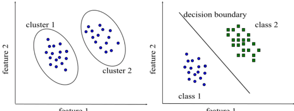
the similar objects into same groups [8, 9]. This is the scenario shown in Figure 1.1(a). An illustration of clustering on two dimensional feature space is given in Figure 1.2(a) where objects are separated into two clusters. Note that, defining a similarity measure for clustering is one of the crucial steps in unsupervised learning and depending on the similarity measure, cost function and input patterns different clustering algorithms lead to different results.
a b c d e f
Figure 1.1: Scenarios of different input/output feature availability (Extended from [1]). Rows correspond to objects/instances. Wide boxes are feature matrices, narrow boxes correspond to labels. Available data are represented in blue, missing data that can be queried by a learning algorithm are represented in purple color.
b) Supervised learning: Each object is represented by one set of features and one label. In supervised learning a set of training data is available and classifier/regressor is designed by using this a priori information [8–10]. This is the scenario shown in Figure 1.1(b). If the target label of the problem is continuous then the supervised learning problem is called regression. Otherwise, if the labels have discrete values then the supervised learning problem is called classification. The aim is to find a mapping from input features to output labels and the mapping needs to minimize an appropriate error function on training data. An illustration of classification in two dimensional feature space is given in Figure 1.2(b), where objects are classified into two different classes.
c) Semi-Supervised learning: Some object labels are available however the other parts’ labels are missing and not available. Learning in this case, using both labeled and unlabeled data, is known as semi-supervised learning [11] (Figure 1.1(c)). Detailed description of Semi-Supervised learning methods is given in Chapter 4. Transductive learning is a special case of semi-supervised learning where the unlabeled instances are actually test instances [12]. There are many extensions [13] to semi-supervised learning and some of them based on active learning and Co-training are defined below. Co-training is detailed Section 4.2.
feature 1
feature 2
cluster 1
cluster 2
(a) Unsupervised learning (clustering)
feature 1
feature 2
class 1
class 2
decision boundary
(b) Supervised learning (classification)
Figure 1.2: a) Unsupervised and b) supervised learning algorithms illustration on two dimensional feature space.
d) Active learning of labels: Some object labels are available however the other parts’ labels are missing but can be acquired [14] (Figure 1.1(d)). Any algorithm for the labeled and unlabeled data can be also used for active learning by selecting random points for collecting the labeled data and selecting the remaining part as unlabeled. However the aim of active learning is to outperform such algorithms [10]. Also this approach assumes the availability of an "oracle" that can label the unlabeled data points in the presence of a question. The intention of active learning is to select the most informative unlabeled examples by asking minimum number of questions to the "oracle" [13].
e) Co-training: A number of feature sets are available, but some of the objects have missing labels that cannot be acquired (Figure 1.1e). Co-training algorithm [15] is an iterative algorithm, that trains different classifiers on different feature views and updates these views by labeling the unlabeled data and adding them to the training set during the iterations. Detailed description of Co-training algorithm is given in Chapter 4.
f) Active learning of labels with co-training: A number of feature sets are available, but some of the objects have missing labels that can be acquired by asking questions to an "oracle" (Figure 1.1f).
g) Active learning of features and labels: Some of the features have missing values and some of the objects have not been labeled. However active learning of features and labels can be achieved by asking an "oracle" (Figure 1.1g). More detailed description can be found in [1].
In some applications data samples obtained from various sources may be represented in different multiple ways (or views), for example, web pages can be represented using text, image and video information. The learning problems summarized in Figure 1.1 e), f) and g) work on two different feature views. When multiple feature views are available, instead of training one classifier on the concatenated feature views, using multiple classifier systems can be useful [16]. On the other hand, on high dimensional feature spaces one can obtain different feature views artificially as in Random Subspaces Method (RAS) [17]. The RAS method selects the feature subspaces randomly for classifier ensembles and are shown to perform well using different classifiers such as K-Nearest Neighbors (KNN) [18], decision trees [17], pseudo Fisher linear classifier [19]. However, RAS method may not perform well when there are irrelevant or redundant features.
1.1 Contributions of the Thesis
The main contributions of this thesis are on relevant and non redundant random subspaces for supervised and semi-supervised learning.
1) Relevant Random Subspaces (Rel-RAS) and minimum Redundancy Maximum Relevance Random Subspaces (mRMR-RAS) Algorithms:
Feature selection and classifier ensembles, on both supervised and semi-supervised learning, are crucial problems in pattern recognition. On the other hand, selecting the relevant features and eliminating the redundant ones is a big issue in feature selection [20]. It has been found that selecting the most relevant features may not result in good classification performance [4]. Therefore redundancy among features is also studied [7, 21]. However training one classifier alone on the selected feature subset may not always give good classification accuracy. Besides, depending on the pattern recognition problem one can obtain many feature views and use classifier ensembles. One of the main contributions of this thesis is made on classifier ensembles. Ensemble learning algorithms may benefit from diversity of classifiers used. However, for high dimensional data choosing subspaces randomly, as in Random Subspaces (RAS) algorithm, may produce diverse but inaccurate classifiers. On the other hand, if there are many irrelevant features and redundancy, RAS may produce subspaces of features
that are not suitable for good classification (See Section 3.2 for RAS algorithm). In order to eliminate these problems, we introduce two subspace selection methods for ensemble of classifiers. The first algorithm is the relevant random subspace method which produces relevant random subspaces using the relevance scores of the features obtained by mutual information between features and class labels. The second algorithm is the relevant and non-redundant random subspace selection that modifies the mRMR feature selection algorithm to produce random feature subspaces that are relevant and non-redundant. These feature subspace selection methods are used in Rel-RAS (Relevant Random Subspaces) and mRMR-RAS (minimum Redundancy Maximum Relevance Random Subspaces) supervised algorithms respectively during subspace selection.
2) Relevant Random Subspaces for Co-training (Rel-RASCO) and minimum
Redundancy Maximum Relevance Random Subspaces for Co-training
(mRMR-RASCO) Algorithms:
The use of unlabeled data is a challenging problem. Many algorithms have been proposed to benefit from unlabeled data [12]. It has been shown that using ensemble of classifiers increases the classification performance on semi-supervised learning as well [22, 23]. Co-training is a type of semi-supervised learning that uses unlabeled data on two different feature views. Previously we proposed a classifier combination method for Co-training algorithm [24]. The Co-training algorithm is extended for multiple feature views by Wang et. al. [23] and named as Random Subspace Method for Co-training (RASCO).
The next contribution of the thesis is made on semi-supervised ensemble learning by using the proposed feature subspace selection algorithms. Relevant Random Subspaces for Co-training (Rel-RASCO) and Relevant and Non-Redundant Random Subspaces for Co-training (mRMR-RASCO) algorithms are proposed for semi-supervised learning and they outperform the RASCO [23] algorithm which uses random subspaces for Co-training. The proposed algorithms are compared using the RM-characteristics of feature subspaces on both supervised and semi-supervised learning cases. It is shown that the proposed algorithms are more RM-characteristics in the mean of the classification accuracy.
3) Diversity Analysis of the Classifier Ensembles:
The last contribution of the thesis is on diversity analysis of the classifier ensembles. The analysis of the algorithms are based on KW-Variance diversity measure [2], information theoretic based low order diversity (LOD) [25] and information theoretic scores (ITS) [26]. It is shown that the increase in the ensemble classifier accuracy can be explained with the information theoretic score. On the other hand KW-Variance diversity measure and information theoretic based low order diversity have similar behavior and the performance increase in the ensemble cannot be explained directly with these measures.
The rest of the thesis chapters are organized as follows:
•In Chapter 2, first classifier ensemble methods, namely Bagging, Boosting, Stacked Generalization, Mixture of Experts, Input Decimated Ensembles are summarized and combination methods are given. Next measures of diversity for classifier ensembles and mutual information based classifier ensemble analysis are given.
• Chapter 3 includes the Random Subspaces (RAS), proposed Relevant Random Subspaces (Rel-RAS) and minimum Redundancy and Maximum Relevance Random Subspace (mRMR-RAS) algorithms. Next theoretical analysis of the algorithms is presented. Experimental results on supervised learning are given in terms of accuracy and diversity.
• In Chapter 4, first semi-supervised learning algorithms are summarized. Then RASCO, Rel-RASCO and mRMR-RASCO algorithms are presented and experimental results are given.
• Chapter 5 concludes the thesis by discussing the outcomes and the possible future directions for the work.
2. CLASSIFIER ENSEMBLES AND DIVERSITY
2.1 Classifier Ensembles
During the last decade computational intelligence community started to benefit from different experts to reduce the probability of making mistake [27,28]. Kittler states that in statistical pattern recognition most of the progress has been on modeling probability density function, feature selection and classification context and describes the classifier ensembles as one of the exciting directions [29]. Besides, in pattern recognition, the models that deal with real-world problems have their own limitations and errors [30]. Classifier Ensembles aim to produce accurate recognition results by training several classifiers [31] and combining their outputs by managing the strengths and weaknesses of the classifiers [30]. In literature various terms have been used for the same notions in classifier combination [2], i.e. classifier ensembles have different names, such as, ensemble based systems, mixture of experts, classifier fusion, committee of classifiers, multiple classifier systems [28].
There are many reasons to build ensembles. Dietterich states statistical, computational and representational reasons to construct ensemble based systems [32]. Statistically, with sufficient data different classifiers can be obtained [32] and combining several classifiers may reduce the risk of making the wrong decision [28]. Computationally, when a classifier is stuck in a local optima it may not perform well or some classifiers, such as neural networks, may perform different based on the initial parameters. Hence combining separately trained classifiers may perform better than selecting the best network and eliminating the others. On the other hand, different classifiers trained on the same dataset may perform differently. In the feature space each classifier may have its own region that it performs best. In some applications different types of features (representation/description) can be obtained and different types of classifiers can be trained on each set of features. For example: in person identification, one can obtain face, voice and handwriting information. Also in neurological disorder diagnosis MRI scan, EEG recording, blood test results can be obtained [28]. In addition to different
representations, different training sets recorded at different times and using different features may also be available.
Different taxonomies of classifier ensembles have been suggested in the literature. Kuncheva [2] divides classifier ensemble framework into four parts: instance, feature, classifier and combination levels (see Figure 2.1). Lam [33] categorizes classifier combination methods into multiple, conditional, hierarchical and hybrid topologies. On the other hand, in a recent work, Rokach [34] presents a new taxonomy on classifier ensembles: inducer, combiner, diversity, size and members’ dependency. Please refer to [2, 28, 34] for further information on classifier ensemble taxonomies.
Dataset
X
. . .C
C
C
C
K-1 K 2 1Classifier
Combiner
Data Level Feature Level Classifier Level Combination Level
FS
1FS
KFigure 2.1:General framework of classifier ensembles [2].
In instance level classifier combination, different datasets are bootstrapped from a training dataset and different classifiers are trained. These techniques work well with unstable classifiers [35], such as decision trees, neural networks, where a small change in the dataset, may causes a major change in the hypothesis [32]. Well known ensemble algorithms in instance level combination category are; Bagging [36] and Boosting algorithms [35]. Feature level approach aims to reduce the dimensionality of feature vectors of the base learners in order to reduce the curse of dimensionality. Some of the feature level algorithms are RAS (Random Subspace Method) [17], Input Decimation Approach [37], and Mixture of Experts [2]. Details of the RAS algorithm will be given in the next chapter. In classifier level, different types of classifiers can be used. Classifier decision combination can be either a classifier selection or classifier
combination. In classifier selection a classifier is selected to give the final decision. Classifier ensemble members can be generated either in parallel or sequentially where subsequent classifiers are created based on the preceding classifiers [38]. The next sections summarize some of the well known classifier ensemble algorithms.
2.1.1 Bagging
Bootstrap Aggregation (Bagging) [36] generates multiple versions of a classifier by training individual classifiers on bootstrapped samples of the training set, using them as new learning sets. Each example in each data subset is selected randomly with replacement and each classifier is trained on the average on 63.2 percent of the entire training set [39]. The generated classifiers are aggregated by majority or weighted voting methods. Bagging performs well with unstable algorithms such as decision trees and multilayer perceptrons where small change in the training set creates a large difference in the classifier [39]. Pseudo code of Bagging is given in Algorithm 1. Algorithm 1 Bagging Algorithm
// X =(X1,X2, ...,Xn)be the training dataset with n samples. // Xi: ith training instance(i=1,2, ...,n)and Xi= (xi1,xi2, ...,xid) // d: the dimensionality of training instance
Training:
for k = 1 to K do
Take a bootstrap sample ˆXkfrom X Train classifier Ck using ˆXk
end for Testing:
Given a test instance t Run C1...Ckon the input t
Choose the class with the maximum number of votes as the label of t
2.1.2 Boosting
In boosting methods, at each iteration learning algorithms use a different weighting or distribution for training. The probability of selecting an individual is adapted at each iteration based on the performance of previous classifiers. The weights of misclassified instances are increased at each iteration. Experimental results show that while boosting is sensitive to noise, bagging is effective with noisy data [35]. The most popular boosting algorithm is adaptive boosting (Adaboost) that keeps adding components until
a predetermined error rate on training dataset is reached [40, 41]. The Adaboost.M1 algorithm [28] for multi-class problems is given in Algorithm 2.
Algorithm 2 Adaboost Algorithm
// X =(X1,X2, ...,Xn)be the training dataset with n instances. // Xi: ith training instance(i=1,2, ...,n)and Xi= (xi1,xi2, ...,xid) // d: the dimensionality of training instances
// c: number of classes
// Initialize the probability of selecting ith instance: D1(i) =1/n, i=1,2, ...,n
Training:
for t = 1 to K do
Select a training instance subset ˆXt drawn from the distribution Dt Train classifier Ct using ˆXt
Calculate, et, the error of Ct if et>05 then abort end if βt = et/(1−et) Zt =∑iDt(i)// Normalization constant if Ct(xi) =lithen Dt+1(i) =Dt(i)×βt/Zt else Dt+1(i) =Dt(i)/Zt end if end for Testing:
Given a test instance x Run C1...CK on input x
Obtain total vote for each class j=1,2, ...,c Vj= ∑
t:Ct(x)=lj
log(1/βt)
Choose the class that receives the highest total vote
2.1.3 Mixture of experts
Mixture of Experts is also another layered classifier ensemble algorithm. In this algorithm in the second layer instead of a classifier there is a selector which determines the participation of the classifiers in the final decision. This algorithm was initially proposed for Neural Networks where each Neural Network is responsible for a portion of the feature space [2]. The outputs of each Neural Network are given to a gating network and the outputs of the gating network is the probability of each classifier to participate for decision. The selector uses these probabilities to give the outputs of the examples.
2.1.4 Stacked generalization
Stacked generalization is a layered algorithm that aims to find a mapping between ensemble classifier outputs and original class labels. Thus at the first level the ensemble classifiers receive the data as input and at the second layer the outputs of the classifiers in the first layer are given as inputs [42]. The algorithm works as follows: Specifically the training data is divided into K folds. Each first level classifier Ck is trained on the different K−1 fold of the training data. For each classifier the remaining one fold of the training data is used as a test set. The outputs of the classifiers and their true labels are used as an input for the second layer classifier [28]. The aim is to learn the classifiers that consistently classify instances correctly or incorrectly.
2.1.5 Input decimated ensembles
The aim of the Input Decimated Ensembles is to de-correlate the base classifiers by training them on different subsets of the input features, selected from the ones that are most correlated with a particular class label [37, 43]. In a c class problem, Input Decimation trains c classifiers, each of them corresponds to one class. For each classifier a user determined number of features, having the absolute correlation to the class label are selected. The objective is to get rid of the features that are not related to each class. In [37] Input Decimation results are evaluated over a synthetic dataset and multi-layer perceptrons are used as base classifiers and combination is achieved by averaging.
2.1.6 Classifier combination methods in classifier ensembles
The decisions of the ensemble of classifiers depend on the output of each classifier. The combination of the classifier outputs can be considered under the categories of: combination of abstract level outputs, combination of ranked lists and combination of continuous level outputs [31, 44]. Kuncheva adds one more type, the oracle level, where the output of a classifier for a given example is only known as correct or incorrect [2].
For further information we refer the Kuncheva’s book on classifier combination [2] and [27, 28, 31, 45, 46].
2.1.6.1 Combinations of abstract level outputs
Combination of abstract level outputs consists of the combination methods that use the classifiers whose output is a unique class label. This combination scheme consists of majority vote, weighted majority vote, Bayesian formulation, a Dempster-Shafer theory of evidence, the Behavior-Knowledge Space method [31].
Voting methods:
Since the combination is achieved only on the outputs of the classifiers without training any combiner, majority voting is the simplest method to implement [2, 31]. The output class label of a data point is decided by the major class label obtained by different classifiers. The general majority vote is the special kind of weighted majority vote where each weight is equal. If the classifiers in the ensemble have different accuracies then giving more weights to the accurate classifiers may improve the ensemble accuracy. Weighting can be obtained using a genetic algorithm according to an objective function or the performance of the classifiers on the training dataset [31]. Bayesian combination rule:
Bayesian combination rule finds the weights of classifiers by using their performances on the training dataset. Therefore the confusion matrix of each classifier is used as an indicator for its performance. For a problem with c class possibilities and plus reject option, the confusion matrix size will be c(c+1). Confusion matrices for all classifiers are calculated and based on these matrices using Bayesian formula belief values for each class are obtained. For any input sample, the class whose belief value is the highest is chosen. Formulation and detailed descriptions about the Bayesian combination can be found in [31].
Behavior-Knowledge space:
Bayesian method assumes the conditional independence of the decisions of the classifiers. Behavior-Knowledge Space method also finds the ensemble from the decisions of the classifiers and can be considered as a refinement of the Bayesian method without assuming conditional independence [31]. High order probabilities are computed from the frequencies on the training set. The algorithm keeps the output combination of the classifiers in the training dataset and creates a table from these combinations. During training, the output combinations of the classifiers and correct
labels are kept on the table. The output combinations are assigned to a class based on the maximum true class decision in the training set [47].
2.1.6.2 Combinations of ranked lists
Some classifiers may output order (ranking) of possible class labels [48]. Instead of the best guess of the classifiers they give a complete ranking of the possible classes. Borda count [28], is a ranked lists combination method used to determine the ranking of the experts without training. Variations of Borda count are used in many real life applications; such as European Song Contest (Eurovision), electing officers at certain university senate elections. The class label of the dataset can be obtained by considering all the ranks obtained from different classifiers.
2.1.6.3 Combinations of continuous outputs
These combination schemes deal with the classifiers that output confidence or distance values for each input sample which can usually be accepted as an estimate of the posterior probability of a particular class given an input instance [28]. Basic combination operators used in this scheme are: Maximum, minimum, mean, median, sum and product rules [49] [50].
2.2 Measures of Diversity for Classifier Ensembles
In many pattern recognition problems, it is difficult to obtain a classifier that has a perfect generalization performance. Classifier ensembles aims to train different classifiers and combine their outputs to perform better than a single classifier [28]. Intuitionally, if we have classifiers in an ensemble that make errors on different data points, it is likely to obtain an ensemble superior to a single classifier. If the classifiers in the ensemble make different errors it is probable that they will be corrected in the ensemble. Diversity of a classifier ensemble measures of how likely are classifiers to give different results on the same data point [2]. In general a good ensemble consists of the base classifiers that are as accurate and diverse as possible [38]. Classifier diversity can be achieved using different training datasets, training parameters, classifiers and feature subsets [28]. Most of the popular algorithms such as bagging and boosting provide diversity with generating datasets by re-sampling instances. Similarly with
different initialization parameters, number of layers and etc. Neural Networks may provide diversity in the ensemble. Another way of providing diversity is to use different types of base classifiers such as decision trees, support vector machines and etc.
In literature there are many works to explain the relationship between classifier diversity and accuracy [2, 51–53]. In order to explain this relationship pairwise and non-pairwise diversity measures are proposed [2, 52]. While pairwise diversity is computed between two classifiers, non-pairwise diversity considers the decision of the classifier ensembles. However there is no consensus on what a good measure of diversity should be [52, 53]. Although there are proven connections between diversity and accuracy, in real-world problems there are some doubts on using diversity measures to build classifier ensembles [54].
Commonly used pairwise and non-pairwise diversity measures are given in the following sections [2]:
2.2.1 Pairwise measures
Pairwise diversity measures are simple to compute and evaluated between two classifiers. For K classifiers K(K−1)/2 pairwise measures are computed and the ensemble diversity is obtained by averaging. The pairwise diversity measures are based on the joint output of two classifiers Ciand Ckas shown in Table 2.1 [52].
Table 2.1: The 2x2 relationship between classifiers with probabilities Ckcorrect (1) Ckwrong (0)
Cicorrect (1) a b
Ciwrong (0) c d
Total: a+b+c+d = 1
The Q-statistics: The Q statistics for classifiers Ci and Ck gives positive values if instances are correctly classified by both classifiers and negative otherwise. It’s calculated as follows:
Qi,k=
ad−bc
ad+bc (2.1)
The correlation coefficient (ρ): is defined as the correlation between the outputs of the classifiers: ρi,k= ad−bc p (a+b)(c+d)(a+c)(b+d) (2.2) If the classifiers are uncorrelated,ρ = 0, then maximum diversity is obtained.
The disagreement measure(D): is defined as the probability that the classifiers disagree:
Di,k=b+c (2.3)
The double-fault measure (DF): is defined as the probability that the classifiers are both incorrect:
DFi,k=d (2.4)
2.2.2 Non-pairwise measures
Non-pairwise diversity measures consider the decision of the classifiers in the ensemble. Some of the most commonly applied non-pairwise diversity measures are as follows [2, 25]:
Kohavi-Wolpert Variance (KW) : Kohavi and Wolpert derived a formula for the variability of the predicted class labels for a specific classifier model. Kohavi Wolpert variance diversity is derived from this formula [2]. Let X = (X1,X2, ...,Xn) be the training dataset with n samples. Xi be the d dimensional ith training instance, Xi =
(xi1,xi2, ...,xid)and(i=1,2, ...,n). Let f(Xj)be the number of classifiers that correctly recognizes the Xj, among o total of K classifiers, the KW-variance is computed as follows: kw= 1 nK2 n
∑
j=1 f(Xj)(K− f(Xj)) (2.5)KW and disagreement measures are linearly related to each other [2].
The Entropy Measure (Ent): If half of the classifiers in the ensemble are correct and the rest are wrong then the highest diversity will be obtained. Let yi= [y1i,y2i, ...,yni]T be n dimensional binary vector such that yji =1 if the classifier Ci recognizes Xj
correctly and yji=0 otherwise, i=1,2, ...,K. The highest diversity among classifiers are for a particular Xj is obtained by⌊K/2⌋of votes in y with the same value and the other part K− ⌊K/2⌋with the alternative value. Thus Entropy measure is defined as follows: Ent= 1 n n
∑
j=1 1 K− ⌊K/2⌋min( K∑
i=1 yji,K− K∑
i=1 yji) (2.6)Entropy value varies between 0 and 1. 0 indicates that there is no diversity between classifiers and 1 indicates their complete dependence.
Generalized Diversity(GD): Let Y be a random variable expressing the proportion of classifiers that fail on a randomly drawn object x∈Rn. Let pidenote the probability that Y =i/K. p(i) be the probability that i randomly chosen classifier will fail on randomly chosen x. The GD is defined as:
p(1) = K
∑
i=1 i Kpi, p(2) =∑ K i=1Ki−−11pi, GD=1− p(2) p(1) (2.7)GD varies between 0 and 1. Minimum diversity is obtained when p(2) = p(1) and maximum diversity is achieved when p(2) =0.
Coincident Failure Diversity (CFD): CFD is a modified version of GD and is calculated as: CFD= 0 p0= 1 1 1−p0∑ K i=1KK−−1ipi p0< 1 (2.8)
The maximum value of CFD is 1 and it is achieved when all misclassifications are unique.
2.3 Information Theoretic Analysis of the Classifier Ensembles
Diversity measures introduced in this chapter have been used in many applications. Especially they have been used for classifier selection. However it is observed that maximizing diversity does not always result in successful classifiers [26]. There are also some studies showing that diversity measures are confusing and ineffective [2,54]. Therefore alternative attempts to analyze the classifier ensembles are emerging. Recently Brown in [25] and Meynet and Thiran in [26, 55] examine the classifier
ensembles in an information theoretic view. Information theory has been applied to many fields from communication to biology and machine learning [25]. It has also been used for feature extraction, selection and pattern classification [26].
Brown analyzed the classifier ensembles in an information theoretic view and expanded mutual information among classifiers in an ensemble into accuracy and diversity components [25]. On the other hand Meynet and Thiran analyzed the dependency between classifiers and their accuracies using information theoretic approach by considering classifiers trained on data coming from the same physical distribution [26, 55].
In this thesis first we will give Brown’s information theoretic approach. Then we will relate it with Meynet and Thiran’s approach.
Let X be the dataset, l represent the labels, and C be any classifier. The aim of any classification algorithm is to estimate the labels: ˆl=C(X). Error of any classifier, p(ˆl6=l), is bounded by the following inequalities [25]:
H(l)−I(X ; l)−1
log(|l|) ≤p(ˆl6=l)≤ 1
2H(l|X) (2.9)
Where H(l) is the entropy of l and I(X ; l) is the mutual information between X and l. Details of the entropy and mutual information are given in Appendix B. In order to increase the classification accuracy H(l|X) should be minimized and I(X ; l) maximized. Similarly, in a classifier ensemble with a set of K classifiers, S = {C1,C2, ...,CK} (Ci, represents the output of the classifier and i = 1,2, ...K), mutual information between classifier outputs and class labels, I(C1:K; l), should be
maximized. Shannon mutual information computes the dependency between variable pairs. In order to compute the dependencies between multiple variables, multivariate mutual information, Interaction Information can be used [25]. Then using Interaction Information the ensemble mutual information, I(C1:K; l), can be expanded as follows:
I(C1:K; l) = K
∑
i=1 I(Ci; l)−∑
C⊆S,|C|=2..K I({C}) +∑
C⊆S,|C|=2..K I({C} |l) (2.10)In Equation 10, the first term,∑Ki=1I(Ci; l), is the relevancy of a classifier output to the class label. The second term is a subtractive term independent of the class labels l. It
is the interaction information among the possible subsets of the classifiers and referred as ensemble redundancy. The last term is an additive term, contains the class labels, and is referred to as conditional redundancy. In order to maximize Equation 10, the second term should be minimized while the others are maximized. The summation is obtained over all possible subsets of classifiers and it can be splitted into low-order and high-order diversity terms as follows:
I(C1:K; l) = K
∑
i=1 I(Ci; l)−∑
|C|=2 I({C}) +∑
|C|=2 I({C} |l) −∑
|C|=3 I({C}) +∑
|C|=3 I({C} |l) −. . . +. . . −∑
|C|=K I({C}) +∑
|C|=K I({C} |l) (2.11)This equation can be interpreted as:
I(C1:K; l) =Individual Mutual Information+2-way diversity +3-way diversity +. . .-way diversity
+K-way diversity (2.12)
If the classifiers are statistically independent, then the diversity would be; I(C1:K; l) =
∑K
i=1I(Ci; l). However in real applications it is difficult to obtain independent classifiers. In [25] 3-way and above diversities are omitted and the ensemble mutual information is approximated using only pairwise interactions:
I(C1:K; l)≈ K
∑
i=1 I(Ci; l)− K−1∑
j=1 K∑
k=j+1 I(Cj;Ck) + K−1∑
j=1 K∑
k=j+1 I(Cj;Ck|l) (2.13)Similarly Meynet and Thiran also tried to measure the quality of classifier ensembles with information theoretic perspective [26, 55]. They aimed to design a global score that can be used in different classifier ensembles and avoid the limitations of the traditional diversity based techniques. Thus an empirical information theoretic score (IT S) is given to measure the goodness of K classifier ensembles combined by majority
voting and this score is also used to select optimal ensemble of classifiers. The proposed (IT S) is:
IT S= (1+ITA)3(1+IT D) (2.14)
where ITA is the information theoretic accuracy which is relevance term normalized by the number of classifiers, K, in Equation 13:
ITA= 1 K K
∑
i=1 I(Ci; l) (2.15)IT D is the information theoretic diversity which is the ratio between the number of pairwise classifiers C(K,2)and diversity term in Equation 13:
IT D= K 2 ∑K−1 j=1 ∑ K k=j+1I(Cj;Ck) (2.16)
While ITA aims to favour the most accurate classifiers, the second term in IT S aims to increase the diversity of an ensemble with same ITA. IT S was shown to outperform the diversity based selection techniques while selecting classifiers in an ensemble. Note that the proposed model of IT S is a choice and as will be shown in the experiments other similar modeling approaches can be used [26].
3. SUPERVISED LEARNING USING INFORMATIVE FEATURE SUBSPACES
In supervised learning a set of training data is available and classifiers that aim to minimize error on an unseen test data are designed using this a priori information [8]. In this chapter we assume that we are only given a training dataset and no unlabeled data is available. First we give related work on supervised learning with Random Subspaces (RAS). Then we introduce the Relevant Random Subspaces (Rel-RAS) and minimum Redundancy and Maximum Relevance Random Subspaces (mRMR-RAS) algorithms. Next these algorithms are analyzed using RM-characteristics of feature subspaces. Finally, experimental results on 5 real datasets, a synthetic dataset and a real dataset with added redundant and noisy features are given. In the experiments, diversity analyses of ensembles are given using both Kohavi Wolpert variance and information theoretic analysis.
3.1 Related Work
In the previous chapter we summarized the well known off-the-shelf classifier ensemble algorithms. Bagging and Boosting algorithms are well known classifier ensemble methods work on the instance space. However, these algorithms require large number of instances to perform well. If the number of features are much larger than the number of instances, algorithms that work on feature subspaces may perform better. In this section, we summarize the previous supervised feature ensemble algorithms. One of the most well known algorithms that trains classifiers on randomly selected feature subspaces is the Random Subspaces algorithm [17]. This algorithm is detailed in the next section.
There are also some algorithms that work both on instance and feature spaces. Random Forest [56] is a modified version of Bagging algorithm and it differs from Bagging in the construction of decision trees. For each node of the decision tree, features that split the node are selected from the best features among the randomly selected
feature subset. Rotation Forest [57] is also another algorithm that uses bootstrapped data. First the feature space is randomly divided into subsets and Principal Component Analysis (PCA) is applied on these subsets. The training dataset for a base classifier is obtained by rotating the original dataset using the PCA coefficients. Decision tree is used as a base classifier and Rotation Forest was shown to perform better than Bagging, Adaboost and Random Forest.
Genetic algorithms were also used for feature subset selection in classifier ensembles and they performed well [58]. Opitz [59] proposed a genetic algorithm based feature selection method for classifier ensembles. The algorithm creates the initial classifiers by selecting random feature subsets. Then feature subsets are updated by crossover and mutation operations. The fitness of each member is obtained using the classifier accuracy and diversity. The ensemble is constructed using the most fit individual classifiers. Oliveira et. al. [60] proposed 2-level hierarchical multi-objective genetic algorithm approach for ensemble creation. Where in the first level a set of good classifiers are generated by conducting feature selection and in the second level the best ensemble is searched among the classifiers generated in the previous level. However genetic algorithms need to have enough population size to be successful and their computational complexity is very high.
On the other hand, a number of studies investigated the use of feature selection methods in classifier ensembles. Vale et. al. [61] proposed a class based feature selection method to be used in the classifier ensembles. Important features corresponding to each class are selected and based on these features a classifier becomes responsible for each class. However in this method the system needs at least one classifier to correctly recognize each class. In [62], hill climbing, a genetic algorithm, forward sequential selection and backward sequential selection are considered for ensemble feature selection. These search strategies incorporate different diversity measures in the search of the best feature subsets and employ the same fitness function. It is shown that ensemble feature selection can be sensitive to the diversity criteria and the performance of the diversity measures depend on the data being processed.
In this thesis, the proposed algorithms differ from the ones in previous works in terms of feature subspace selection. Instead of the best features as in most of the previous works, the algorithms proposed in this thesis select features randomly. The probability
![Figure 1.1 : Scenarios of different input/output feature availability (Extended from [1])](https://thumb-us.123doks.com/thumbv2/123dok_us/8996748.2797500/26.892.174.664.299.456/figure-scenarios-different-input-output-feature-availability-extended.webp)
![Figure 2.1 : General framework of classifier ensembles [2].](https://thumb-us.123doks.com/thumbv2/123dok_us/8996748.2797500/32.892.144.691.409.764/figure-general-framework-of-classifier-ensembles.webp)