Smoothing technique for nonsmooth composite
minimization with linear operator
Quang Van Nguyen∗, Olivier Fercoq†, and Volkan Cevher∗ ∗Laboratory for Information and Inference Systems (LIONS)
´
Ecole Polytechnique F´ed´erale de Lausanne (EPFL), Switzerland
†T´el´ecom ParisTech, Institut Mines-T´el´ecom Paris, France [email protected], [email protected]
Abstract
We introduce and analyze an algorithm for the minimization of convex functions that are the sum of differentiable terms and proximable terms composed with linear operators. The method builds upon the recently developed smoothed gap technique. In addition to a precise conver-gence rate result, valid even in the presence of linear inclusion constraints, this new method allows an explicit treatment of the gradient of differentiable functions and can be enhanced with line-search. We also study the consequences of restarting the acceleration of the algorithm at a given frequency. These new features are not classical for primal-dual methods and allow us to solve difficult large scale convex optimization problems. We numerically illustrate the supe-rior performance of the algorithm on basis pursuit, TV-regularized least squares regression and L1 regression problems against the state-of-the-art.
Key words. composite minimization, forward-backward, multivariate minimization, atomiza-tion energies predicatomiza-tion, smoothing technique, total variaatomiza-tion regularizaatomiza-tion.
Mathematics Subject Classifications (2010)47H05, 49M29, 49M27, 90C25
1
Introduction
Nonlinear and non-smooth convex optimization problems are widely presented in many disciplines, including signal and image processing, operations research, machine learning, game theory, eco-nomics, and mechanics. In this paper, we consider the following problem.
Problem 1.1 Let H and G be real Hilbert spaces, letM:H → G be a bounded linear operator, and let f: H → R, g: H → (−∞,+∞] and h:G → (−∞,+∞] be proper, closed lower semi-continuous convex functions wherefis moreover assumed to haveLf-Lipschitz gradient. Consider
the following generic convex minimization problem
F?= min
x∈H
f(x) +g(x) +h(M x) (1.1)
under the assumption that its set of minimizersP? is non-empty.
Following [1, Definition 19.11], if we suppose that∅ 6=M(dom(f+g))∩domh=M(domg)∩ domhand setF:H × G: (x, y)7→f(x) +g(x) +h(M x−y)then Problem1.1becomes the primal problem associated toFand its associated dual problem is
G?= max y∈G G(y) = min x∈H f(x) +g(x) + M x, y −h∗(y) , (1.2) where domf = x∈ H
f(x)<+∞ is the domain of f and h∗: G → (−∞,+∞] : y 7→ max ¯ y∈G ¯ y, y
−h(¯y)is the Fenchel-Moreau conjugate function ofh. In this case, [1, Corollary 19.19] states that the set of solutionD? to (1.2) is non-empty, and furthermore, a pointx? ∈ His inP? if
and only if there existsy? ∈D?such that(x?, y?)is a saddle point of the Lagrangian function
L: (x, y)7→f(x) +g(x) +M x, y−h∗(y). (1.3)
A particular case of Problem 1.1is when h = ιK(· −c) with c ∈ G, is the indicator function of a non-empty closed convex subsetK⊂ G, i.e.,
ιK:G →(−∞,+∞] :y7→
(
0, ify∈K,
+∞, otherwise. (1.4)
In this case, Problem1.1reduces to the following constrained minimization problem
min
x∈H
f(x) +g(x) : M x−c∈K , (1.5)
and furthermore, ifg=ιX for someX ⊂ H,
min
x∈H
f(x) : x∈X such thatM x−c∈K . (1.6)
A traditional approach for smooth minimization problems is the gradient descent algorithm together with its accelerated version. This idea has already been adapted for nonsmooth composite minimization problem by linearizing the smooth term before minimizing. For instance, if h = 0, then Problem 1.1 can be solved by FISTA (in other words, an accelerated forward-backward algorithm) [3, 5], and this approach can be generalized to the case where h is with Lipschitz gradient. If furthermore,h=ι{c}for somec∈ G, then various of alternating direction optimization methods (ADMM) [7] can be used. A linearization technique is recently combined with ADMM in [15] to tackle such cases. However, in the general case, we need a special treatment of h(M x).
For instance, we may compute approximations to the proximal operator of(x7→g(x) +h(M x))as in [2]. We obtain an algorithm with a nested loop for this proximal operator computation. Provided we are able to control theaccuracy of the inner loop, we can obtain convergence rates.
Another possibility is to consider primal-dual splitting. By interpreting the optimization prob-lem 1.1as a saddle point problem, we can derive methods updating primal and dual variables at each iteration, without any nested loop. A primal-dual method able to deal with our composite framework was given in [6,14].
A powerful smoothing framework was first introduced in [9], which can also be applied to solve Problem 1.1. The main idea isto consider a smoothed approximation to the nonsmooth function
hand minimize the resulting problem using an accelerated forward-backward algorithm. This ap-proach has been improved (for the case f = 0) in [13] as follows. Instead of considering a fixed smoothed approximation to the nonsmooth functionh, the authors set up a homotopy strategy by considering a decreasing smoothing parameter. In doing so, they obtain improved convergence characterizations, and,more importantly, they prove finite-time convergence rates in terms of func-tion value and infeasibility. Indeed, these rates are difficult to obtain in the constrained case when approximately solving the proximity operator or considering classical primal-dual algorithms.
In this paper, we build on this latter, homotopy-based smoothing technique to tackle the more general composite framework, i.e., Problem1.1. In this scenario, to apply the technique of [9] as in [13], it would require the computation of the proximity operator off+gwhich is generally not easy even the case where one knows how to compute the proximity operators offandgseparately. One of our goals is to avoid this computational difficulty by using the smoothness. The second non-smooth part is then smoothed using the idea of [9]. To see this, let us rewrite the objective function of (1.1) as follows F(x) :=f(x) +g(x) +h(M x) =f(x) +g(x) + max y∈G M x, y −h∗(y), (1.7)
Instead of minimizing F, we first smooth one of its nonsmooth parts, says h, controlled by a smoothness parameterβ∈]0,+∞[and then minimize
Fβ(x) :=f(x) +g(x) + max y∈G
M x, y−h∗(y)−βq(y) , (1.8)
with a suitable strongly convex functionq:G →(−∞,+∞]. We then use the accelerated forward-backward scheme to design algorithms that maintain the decrease of the approximated objective function in the sense that
(∀k∈N) Fβk+1(¯x
k+1)−F?
6(1−τk) Fβk(¯x
k)−F?
+ψk, (1.9)
where (¯xk)k∈N and the parameters are generated by the algorithm with (τk)k∈N ⊂ [0,1)N and
(max(ψk,0))k∈N tends to zero. We will also simultaneously update the βk+1 parameter to zero to achieve an O(1/k) convergence rate. Our approach allows us to consider features that were introduced initially for unconstrained optimization like line-search or the balance of computational power between the steps of the algorithm.
The rest of the paper is organized as follow. In Section2 we revise some technical facts. The main result is presented in Section3. Numerical evidence is placed in Section4.
Notation. The Hilbert spaces H and G are equipped with their respective norms and inner products that we will both denote byk · kand
·,·
respectively. A positive definite linear operator
S onG, i.e., ∃σ ∈ ]0,+∞[ such that (∀y ∈ G)
y, Sy
> σkyk2, induces a norm (∀y ∈ G kyk
S = q
y, Sy. Given a proper, closed, lower semi-continuous convex functionf: H →(−∞,+∞], we denote by int domf the interior of domf and by
∂f:x7→
v ∈ H
(∀y∈ H)f(x) +
y−x, v6f(y) (1.10)
the subdifferential off. Iff is differentiable, then we use∇f for its gradient and in this case we say thatf hasLf-Lipschitz gradient with respect to normk · kS if
(∀x∈ H)(∀y∈ H) f(x)6f(y) + x−y,∇f(y) +Lf 2 kx−yk 2 S. (1.11)
Finally, we say thatf isµ-strongly convex onHwith respect tok · kS if
(∀x∈ H)(∀y∈ H)(∀v∈∂f(y)) f(x)>f(y) + x−y, v + µ 2kx−yk 2 S. (1.12)
Without indicating the norm, we are assuming that Lipschitz continuity or strong convexity is with a Hilbertian norm.
2
Preliminaries
In this section we revise some basic facts about the proximity operators and functions, and further-more, the smoothing technique for non-smooth functions using the Fenchel-Moreau conjugate. In the optimization, the following notion of the proximity operators is widely used.
Definition 2.1 [1, Definition 12.23] Letg:H →(−∞,+∞]be a proper closed lower-semicontinuous convex function. The proximity operator ofgis
proxg:H → H:x7→argmin
z∈H
g(z) +1
2kz−xk
2. (2.1)
Lemma 2.2 [1, Proposition 12.26]Letg:H →(−∞,+∞]be a proper closed lower semi-continuous
convex function, letγ ∈]0,+∞[, letx∈ Hand letp=proxγg(x). Then, it holds that
(∀z∈ H) γ−1
z−p, x−p
+g(p)6g(z). (2.2)
The following smoothing technique using the Fenchel-Moreau conjugate and the proximity functions is from [9].
Definition 2.3 Let h: G → (−∞,+∞]be a convex function, let β ∈ ]0,+∞[, let S be a positive definite linear operator onG and lety˙∈ G. Theβ-smooth approximation ofhis
hβ(·; ˙y) :G →(−∞,+∞] :y7→max ¯ y∈G y,y¯−h∗(¯y)−β 2ky¯−y˙k 2 S . (2.3)
Set (∀y ∈ G) yβ∗(y; ˙y) =argmax ¯ y∈G y,y¯−h∗(¯y)−β 2ky¯−y˙k 2 S. (2.4)
For instance, ifS=I then
(∀y ∈ G) yβ∗(y; ˙y) =proxβ−1h∗ β−1y+ ˙y
. (2.5)
We summarize important properties of the smooth approximation in the following lemma which will be a crucial key in the analysis of our algorithm.
Lemma 2.4 Leth:G →(−∞,+∞]be convex, letSbe a positive definite linear operator onGand let
˙
y∈ G. Consider the smooth approximations ofh
(∀β ∈]0,+∞[) hβ(·; ˙y) :G →(−∞,+∞] :y7→max ¯ y∈G y,y¯ −h∗(¯y)−β 2ky¯−y˙k 2 S . (2.6)
Then the following hold:
(i) Denote˜h: (β, y)7→hβ(y; ˙y). Then we have the following:
(a) ˜his differentiable with respect to both variables and
(∀y∈ G)(∀β ∈]0,+∞[) ∂˜h ∂β(β, y) =− 1 2ky ∗ β(y; ˙y)−y˙k2S =− 1 2k∇hβ(y; ˙y)−y˙k 2 S. (2.7)
(b) ˜his convex with respect to first variable and
(∀y∈ G)(∀β¯6β˜) ˜h( ¯β, y)6˜h( ˜β, y)−( ˜β−β¯)∂ ˜ h ∂β( ¯β, y) = ˜h( ˜β, y) +β˜−β¯ 2 k∇hβ¯(y; ˙y)−y˙k 2 S. (2.8)
(ii) Let β ∈ ]0,+∞[. Then the function y 7→ hβ(y; ˙y) is well-defined on G. It is convex with β1
-Lipschitz gradient in the normk · kS−1 and furthermore,
(∀(¯y,yˆ)∈ G2) hβ(ˆy; ˙y)+ ¯ y−y,ˆ ∇hβ(ˆy; ˙y) 6hβ(¯y; ˙y)− β 2k∇hβ(ˆy; ˙y)−∇hβ(¯y; ˙y)k 2 S. (2.9)
(iii) The following inequality holds:
(∀(y,yˆ)∈ G2)(∀β ∈]0,+∞[) hβ(ˆy; ˙y) + y−y,ˆ ∇hβ(ˆy; ˙y) 6h(y)−β 2k∇hβ(ˆy; ˙y)−y˙k 2 S. (2.10)
(iv) For all(β, τ)∈]0,+∞[2and for all(¯y,yˆ)∈ G2, one has
06k(1−τ)(∇hβ(ˆy; ˙y)− ∇hβ(¯y; ˙y) +τ(∇hβ(ˆy; ˙y)−y˙)k2S
= (1−τ)k∇hβ(ˆy; ˙y)− ∇hβ(¯y; ˙y)k2S+τk∇hβ(ˆy; ˙y)−y˙k2S−τ(1−τ)k∇hβ(¯y; ˙y)−y˙k2S.
(2.11)
Proof. (i)(a) As there is a unique minimizer to the problem defining hβ(·; ˙y), the function is
differentiable with respect toβandy.
(i)(b)The functionβ 7→hβ(y; ˙y)is convex as it is a maximum of functions, which are linear in
β indexed byy andy˙. The rest follows by convexity and the first point.
(ii)By the same arguments as in [9, Theorem 1] we deduce that the function y 7→ hβ(y; ˙y)is
convex and finite onG. It also has 1β-Lipschitz gradient in the normk · kS−1. (2.9) is the cocoercivity
inequality for convex functions with Lipschitz gradient. We provide the proof for completeness. Defineφ(z) =hβ(z; ˙y)− h∇hβ(ˆy; ˙y), zi. The functionφis convex, its minimum is attained atyˆand
it has a 1
β-Lipschitz gradient in the normk · kS−1. Hence
φ(ˆy)6φ(¯y−β−1S∇φ(¯y))6φ(¯y)−β−1h∇φ(¯y), S∇φ(¯y)i+β 2kβ
−1S∇φ(¯y)k2
S−1.
We get the result because∇φ(¯y) =∇hβ(¯y; ˙y)− ∇hβ(ˆy; ˙y).
(iii)Let(¯y,yˆ)∈ G2 andβ ∈]0,+∞[and sety∗
β =y ∗ β(ˆy; ˙y) =∇hβ(ˆy; ˙y). We have hβ(ˆy; ˙y) + y−y,ˆ ∇hβ(ˆy; ˙y) =y, yˆ β∗−h∗(yβ∗)−β 2ky ∗ β−y˙k2S+ y−y, yˆ ∗β = y, yβ∗ −h∗(yβ∗)−β 2ky ∗ β−y˙k2S 6max ¯ y∈G y,y¯ −h∗(¯y) −β 2ky ∗ β−y˙k2S 6h(y)−β 2k∇hβ(ˆy; ˙y)−y˙k 2 S. (2.12)
(iv)This follows from the classical equality
k(1−τ)a+τ bkS2 = (1−τ)kak2S+τkbk2S−τ(1−τ)ka−bk2S. (2.13)
3
Main results
3.1 Presentation of the algorithms
In this section, we design new algorithms to solve Problem1.1based on the smoothing technique introduced in the previous section. Consider the setting of Problem1.1. We fix a positive definite
linear operatorS onG and a pointy˙ ∈ G. We will need the operator norm ofM defined as
kMkS−1 = sup
x6=0
kM xkS−1
kxk
Our first algorithm is given as Algorithm1. Algorithm 1Linearized ASGARD
1: Inputs: τ0= 1,β0 >0,x¯0∈ H,x˜0 ∈ H. 2: fork= 0,1, . . .do 3: xˆk= (1−τk)¯xk+τkx˜k 4: βk+1 = 1+βkτk andBk+1=Lf+ kMk2 S−1 βk+1 5: vk=M∗yβ∗ k+1(Mxˆ k; ˙y) 6: x˜k+1 =prox 1 τkBk+1g ˜ xk− 1 τkBk+1(∇f(ˆx k) +vk) 7: x¯k+1 = ˆxk+τk(˜xk+1−x˜k) = (1−τk)¯xk+τkx˜k+1
8: Find the unique positiveτk+1 such that Bk+1−Lf
Bk+1
τk3+1+τk2+1+τk2τk+1−τk2= 0
9: end for 10: return x¯k+1
Remark 3.1 Let us consider problem (1.5) with K = {0}. Recent paper [15] proposed a com-bination of linearizing technique and alternating direction of multipliers methods to solve (1.5) in which they obtained the O(1/k)-rate (ergodic) convergence for fixed parameters andO(1/k2)
with adaptive parameters. Recall that in this caseh = ι{c} and henceyβ∗k+1(Mxˆ
k)in the step5 of
Algorithm1(withy˙= 0andS=I) becomes
yβ∗k+1(Mxˆk) =proxβ−1 k+1h∗(β −1 k+1Mxˆ k) =β−1 k+1 Mxˆ k−prox βk+1h(Mxˆ k) =β−k+11 Mxˆk−c, (3.1)
where we used Moreau’s decomposition [1, Theorem 14.3]. Hence, for problem (1.5) with K = {0}, our Algorithm1is non-augmented Lagrangian version of [15, Algorithm 1] where in Step6, instead of using linearized augmented Lagrangian as [15], we only used linearization off+gand hence this step only requires the computation of proximity ofg. We also note that the update rule for parameters of [15] is different from ours.
For some problems, for instance whenfencodes some data-fitting term, computing∇f requires much more computational power than proxh∗ or proxg. To circumvent this issue and concentrate
on the non-smoothness of the objective, we propose Algorithm2, a variant of the standard ASGARD in which we use old gradients.
Algorithm 2Linearized ASGARD with old gradients 1: Inputs: τ0= 1,β0 >0,x¯0∈ H,x˜0 ∈ H,xˆˆ0∈ H,δ >0andσ >0. 2: fork= 0,1, . . .do 3: xˆk= (1−τk)¯xk+τkx˜k 4: βk+1 = 1+βkτ k andBk+1=Lf+ kMk2 S−1 βk+1 5: vk=M∗y∗ βk+1(Mxˆ k; ˙y) 6: x˜k+1 =prox 1 τkBk+1g ˜ xk− 1 τkBk+1(∇f(ˆxˆ k) +vk) 7: x¯k+1 = ˆxk+τk(˜xk+1−x˜k) = (1−τk)¯xk+τkx˜k+1 8: if 12kx¯k+1−xˆˆkk2−1 2kx¯k+1−xˆkk26σ τ2 kBk+1 Lf 2+δ then 9: xˆˆk= ˆxˆk−1 10: else 11: xˆˆk= ˆxk
12: Goto6and recompute(¯xk+1,x˜k+1)with the true gradient.
13: end if
14: Find the unique positiveτk+1 such that Bk+1−Lf
Bk+1
τk3+1+τk2+1+τk2τk+1−τk2= 0
15: end for 16: return x¯k+1
Remark 3.2 Let us consider the case whenxˆˆk+1= ˆxk. We have 1 2kx¯ k+2−xˆˆk+1k2−1 2kx¯ k+2−xˆk+1k2 =hx¯k+2−xˆˆk+1+ ˆxk+1 2 ,xˆ k+1−xˆˆk+1i =hτk+1(˜xk+2−x˜k+1)− ˆ ˆ xk+1−xˆk+1 2 ,xˆ k+1−xˆˆk+1i ˆ xk+1−xˆˆk+1 = ˆxk+1−xˆk=τk+1(˜xk+1−xˆk) +τk(1−τk+1)(˜xk+1−x˜k)
and so assuming boundedness of the iterates, 21kx¯k+2−xˆˆk+1k2−1
2kx¯k+2−xˆk+1k2 is at most of the
order ofτk2 ∈ O(1/k2). It is thus likely that it may sometimes be smaller than σ τ
2 kBk+1 Lf 2+δ ifδis small enough.
The last variant of our method is Algorithm3. It is equipped with a line search inspired by the line search for the accelerated universal gradient method [10]. It is particularly useful when the Lipschitz constant of∇f is difficult to estimate. Moreover, it automatically adapts to the case when
his smooth by preventing the current estimate of the Lipschitz constantBk+1to increase to infinity.
Note that because of the line search test on Step 12, the use of old gradients is not compatible with this line search. Unlike the line search of Malitsky et al [8], the goal here is not only to adaptively estimatekMk2but also the wholeL
f+kMk2/β. Our line search is more computationally
demanding but may take profit of some local smoothness of the nonsmooth function h. Algorithm 3Linearized ASGARD with line search
1: Inputs: τ0= 1,β0 >0,x¯0∈ H,x˜0 ∈ H,B0 6a(Lf + kMk2 S−1 β0 ),a >1. 2: fork= 0,1, . . .do 3: Bk+1=a−1Bk 4: repeat 5: Bk+1=aBk+1
6: Find the unique positiveτksuch that τ12−τk kBk+1 = 1 τ2 k−1Bk (exceptτ0 = 1) 7: xˆk= (1−τk)¯xk+τkx˜k 8: βk+1= 1+βkτk 9: vk=M∗yβ∗ k+1(Mxˆ k; ˙y) 10: x˜k+1=prox 1 τkBk+1g ˜ xk−τ 1 kBk+1(∇f(ˆx k) +vk) 11: x¯k+1= ˆxk+τk(˜x+−x˜k) = (1−τk)¯xk+τkx˜k+1 12: until f(¯xk+1) +hβk+1(Mx¯ k+1; ˙y) 6 f(ˆxk) +h βk+1(Mxˆ k,y˙) +h∇f(ˆxk) + vk,x¯k+1 −xˆki + Bk+1 2 kx¯ k+1−xˆkk2 13: end for 14: return x¯k+1
3.2 Convergence of the parameters to 0
Lemma 3.3 Let(τk)k∈N,(βk)k∈Nand(Bk+1)k∈Nbe the positive sequences determined by Algorithm1. Then the following hold:
(∀k∈N\{0}) 1−τk τk2Bk+1 = 1 τk2−1Bk . (3.2) Furthermore, (∀k∈N) 1 k+ 1 6τk6 2 k+ 2, βk6 β0 k+ 1 and τ 2 kBk+16 τ02B1 k+ 1. (3.3)
Proof. First it follows from Step4of Algorithms1and2that
(∀k∈N\{0}) Bk+ (Bk−Lf)τk Bk+1 = Lf + kMk2 S−1 βk + kMk2 S−1 βk (βk−βk+1) βk+1 Lf+ kMk2 S−1 βk+1 = Lf + kMk2 S−1 βk+1 Lf + kMk2 S−1 βk+1 = 1, (3.4)
and Step8yields
(∀k∈N\{0}) 1 −τk τk2Bk+1 = 1 τk2−1Bk Bk+ (Bk−Lf)τk Bk+1 = 1 τk2−1Bk . (3.5)
Next the definitions of(τk)k∈Nand(βk)k∈Nimply that
(∀k∈N) αk+1τk3+1+τk2+1+τk2τk+1−τk2= 0 and (1 +τk)βk+1 =βk, (3.6) where we define (∀k∈N) αk+1 = Bk+1−Lf Bk+1 ∈ [0,1]. (3.7)
Forα∈ [0,1]andτ >0, let us consider the following cubic function
(∀t∈R+) P(t) =αt3+t2+τ2t−τ2. (3.8)
On the one hand, since(∀t >0)P0(t) >0andP(0) =−τ2 <0andP(1) =α+ 1>0, we deduce thatP has a unique roott+ ∈]0,1[. On the other hand, let us define
(∀t∈R+) Q(t) =t2+τ2t−τ2. (3.9)
Then(∀t∈R+) Q(t)6P(t), and in particular,P(t?)>Q(t?) = 0 =P(t+), wheret? is the unique
positive root of Q, that is t? = (−τ2+√τ4+ 4τ2)/2. As P is nondecreasing on ]0,+∞[, we get t+6t?. Consequently, sinceτ0 >0, we deduce that(τk)k∈Nis well-defined and furthermore,
(∀k∈N) τk+1 6
−τk2+ q
τk4+ 4τk2
2 . (3.10)
This inequality and induction onk∈Neasily yields
(∀k∈N) τk6
2
Now the two equalities in (3.6) imply that (∀k∈N) (βk−βk+1) =βk+1τk and τk2 =τk2+1 1 +αk+1τk+1 1−τk+1 < τk2+11 +τk+1 1−τk+1 . (3.12)
We show by induction that
(∀k∈N) τk>
1
k+ 1. (3.13)
Note thatτ0 = 1 > 0+11 . Suppose that there exists k0 ∈ Nsuch that τk0 >
1
k0+1 and thatτk0+1 <
1
k0+2. Then we deduce from (3.12) that
1 (k0+ 1)2 6 τk20 < τk20+11 +τk0+1 1−τk0+1 < 1 (k0+ 2)2 1 +k1 0+2 1− 1 k0+2 = 1 (k0+ 2)2 k0+ 2 k0+ 1 (3.14) which is equivalent to(k0+ 2)2 <(k0+ 1)(k0+ 2)which never happens. Hence, (3.13) holds true.
We then deduce from induction that
(∀k∈N) βk+1 = βk 1 +τk 6 βk k+ 1 k+ 2 6β0 k Y l=0 l+ 1 l+ 2 = β0 k+ 2. (3.15)
Of courseβ06 0+1β0 and hence,
(∀k∈N) βk6
β0
k+ 1. (3.16)
It again follows from induction and from (3.13) that
(∀k∈N) τk2Bk+1 = (1−τk)τk−1Bk =. . .= k Y l=1 (1−τl)τ02B1 6 k Y l=1 1− 1 l+ 1 τ02B1 =τ02B1 k Y l=1 l l+ 1 = B1 k+ 1. (3.17)
The convergence of Algorithm3is based on the following asymptotic property of parameters. Lemma 3.4 Let(τk)k∈N,(βk)k∈Nand(Bk+1)k∈Nbe the positive sequences determined by Algorithm3.
Then(∀k∈N)τk6 k+22 and (∀k∈N) β0 2B1 τk2Bk+16βk+16 1 2 3aβ0 B1 τk2Lf + r (3aβ0 B1 τ2 kLf)2+ 12a β0 B1 τ2 kkMk2S−1 ∼ r 3aβ0 B1 kMkS−1τk=O 1 k . (3.18)
Proof. For every k ∈ N, since Lemma 2.4 (ii) states that the function y 7→ hβk+1(y; ˙y) has
1
βk+1-Lipschitz gradient, we deduce that the function x 7→ f(x) +hβk+1(M x; ˙y) hasLf +
kMk2 S−1
βk+1
-Lipschitz gradient and thus, in Algorithm3, when the line search terminates, one necessarily has
Bk+1 6a(Lf +
kMk2 S−1
βk+1 ). Now we deduce from the definition of(τk)k∈Nthat
(∀k∈N) τk2Bk+1 = (1−τk)τk2−1Bk =τ02B1
k Y
l=1
(1−τl), (3.19)
so we need to study the bounds for(τk)k∈N. We now prove by induction that
(∀k∈N) τk6
2
k+ 2. (3.20)
We clearly have τ0 = 1 6 0+22 . Suppose that there existsk0 ∈ N\{0} such thatτk0−1 6
2 k0+1 and thatτk0 > 2 k0+2. Then, asBk0+1 >Bk0, we have 1−τk0 τk2 0 = Bk0+1 τk2 0−1Bk0 > τ21 k0−1
. This would lead to
k02+ 2k0+ 1 4 = (k0+ 1)2 4 6 1 τk2 0−1 6 1−τk0 τk2 0 < (k0+ 2) 2 4 − k0+ 2 2 = k20+ 2k0 4 . (3.21)
This contradiction proves (3.20). Since we have
(∀k∈N) βk+1 =β1 k Y l=1 1 1 +τl =β1 Qk l=1(1−τl) Qk l=1(1−τl2) = β0 2 Qk l=1(1−τl) Qk l=1(1−τl2) , (3.22) and since (∀k∈N) 1> k Y l=1 (1−τl2)> k Y l=1 1− 4 (l+ 2)2 = (k+ 4)(k+ 3)2.1 (k+ 2)(k+ 1)4.3 > 1 6, (3.23) we get (∀k∈N) β0 2 k Y l=1 (1−τl)6βk+1 63β0 k Y l=1 (1−τl). (3.24) Therefore, (∀k∈N) β0 2 τk2Bk+1 B1 6 βk+163β0 τk2Bk+1 B1 (3.25) Since(∀k∈N)Bk+1 6a(Lf + kMk2 S−1 βk+1 ), it follows that (∀k∈N) βk2+1−3a β0 B1 τk2 Lfβk+1+kMk2S−1 60, (3.26)
which implies that (∀k∈N) βk+1 6 1 2 3a β0 B1 τk2Lf+ s 3aβ0 B1 τk2Lf 2 + 12aβ0 B1 τk2kMk2 S−1 ! ∼ r 3aβ0 B1 kMkS−1τk =O 1 k (3.27) and hence, (∀k∈N) τk2Bk+1 6 2B1 β0 βk+1=O 1 k . (3.28) 3.3 Speed of convergence
The convergence theorem is based on the decrease of the smoothed optimality gap. We prove in Proposition 3.5that for every iterationk ∈ N,Fβk+1−F
? decreases asO(1/k). Then, using [13,
Lemma 2.1] and the decrease of the smoothness parameter to 0, we get the speed of convergence in function value and infeasibility.
Proposition 3.5 Consider the setting of Problem1.1. Let(¯xk)
k∈Nbe generated by the ASGARD
vari-ants (Algorithms1,2,3) and define
(∀k∈N) Fβk:x7→f(x) +g(x) +hβk(M x; ˙y). (3.29)
Then forx? ∈P?, we have:
(∀k∈N) Fβk+1(¯x k+1)−F? 6 B1 2(k+1)kx?−x˜0k2, for Algorithm1, B1 k+1 1 2kx?−x˜0k2+σ B1 2Lf 1+δ ζ(1 +δ) , for Algorithm2, B1βk+1 β0 kx ?−x˜0k2 =O kx?−x˜ 0k2 k , for Algorithm3, (3.30) whereζ(s) =P+∞ i=0 (i+1)1 s.
Proof. First we note that the arguments for Algorithms 1 and 3 are similar to those of
Algo-rithm2by setting(∀k∈N) ˆxˆk= ˆxk. We therefore prove the convergence for Algorithm2. Now let us fixx? ∈P?. Then, we have
(∀k∈N) f(¯xk+1) +hβk+1(Mx¯ k+1; ˙y) 6f(ˆxˆk) +hβk+1(Mxˆ k; ˙y) + ¯ xk+1−xˆˆk,∇f(ˆxˆk) +x¯k+1−xˆk, vk)+Lf 2 kx¯ k+1−xˆˆkk2+ kMk2S−1 2βk+1 kx¯k+1−xˆkk2. (3.31)
Becausegis convex and because Algorithm2yield(∀k∈N) ¯xk+1= (1−τk)¯xk+τkx˜k+1, we get
(∀k∈N) g(¯xk+1)6(1−τk)g(¯xk) +τkg(˜xk+1). (3.32)
It now follows from Lemma2.2that
(∀k∈N) g(˜xk+1)6g(x?)−τkBk+1 x?−x˜k+1,x˜k−x˜k+1−τk−1Bk−+11 ∇f(ˆxˆk) +vk =g(x?)−τkBk+1 x?−x˜k+1,x˜k−x˜k+1+x?−x˜k+1,∇f(ˆxˆk) +vk =g(x?) + x?−x˜k+1,∇f(ˆxˆk) +vk + τkBk+1 2 kx ?−x˜kk2−τkBk+1 2 kx ?−x˜k+1k2−τkBk+1 2 kx˜ k+1−x˜kk2. (3.33)
In turn, we obtain from (3.31) and the fact that(∀k∈N) ¯xk+1−xˆˆk = ˆxk−xˆˆk+τk(˜xk+1−x˜k)that
(∀k∈N) Fβk+1(¯x k+1)6f(ˆxˆk) +h βk+1(Mxˆ k; ˙y) + (1−τ k)g(¯xk) +τkg(x?) +τk x?−x˜k, vk + ˆ xk−xˆˆk+τk(x?−x˜k),∇f(ˆxˆk) +τ 2 kBk+1 2 kx ?−x˜kk2 −τ 2 kBk+1 2 kx ?−x˜k+1k2+Lf 2 kx¯ k+1−xˆˆkk2−Lf 2 kx¯ k+1−xˆkk2. (3.34) Since Algorithm2yield(∀k∈N)τk(ˆxk−x˜k) = (1−τk)(¯xk−xˆk), we have
(∀k∈N) τk(x?−x˜k) =τk(x?−xˆk) + (1−τk)(¯xk−xˆk), (3.35) and hence, (∀k∈N) τk x?−x˜k, vk=τk x?−xˆk, vk+ (1−τk) ¯ xk−xˆk, vk. (3.36)
Moreover, since(∀k∈N) ˆxk−xˆˆk+τk(x?−x˜k) =τk(x?−xˆˆk) + (1−τk)(¯xk−xˆˆk), we get
(∀k∈N) ˆ xk−xˆˆk+τk(x?−x˜k),∇f(ˆxˆk) =τk x?−xˆˆk,∇f(ˆxˆk) + (1−τk) ¯ xk−xˆˆk,∇f(ˆxˆk) . (3.37) Becausef is convex, (1.10) yields
(∀k∈N) f(ˆxˆk)+x¯k−xˆˆk,∇f(ˆxˆk)6f(¯xk) and f(ˆxˆk)+x?−xˆˆk,∇f(ˆxˆk)6f(x?), (3.38) and hence, we derive from (2.9) that
(∀k∈N) f(ˆxˆk) +hβk+1(Mxˆ k; ˙y) + ¯ xk−xˆˆk,∇f(ˆxˆk) + ¯ xk−xˆk, vk 6f(¯xk) +hβk+1(Mx¯ k; ˙y)−βk+1 2 k∇hβk+1(Mxˆ k; ˙y)− ∇h βk+1(Mx¯ k; ˙y)k2 S. (3.39)
and from (2.10) that
(∀k∈N) f(ˆxˆk) +hβk+1(Mxˆ k; ˙y) + x?−xˆˆk,∇f(ˆxˆk)+x?−xˆk, vk 6f(x?) +h(M x?)−βk+1 2 k∇hβk+1(Mxˆ k; ˙y)−y˙k2 S. (3.40)
On the other hand, we deduce from (2.8) that (∀k∈N) hβk+1(Mx¯ k; ˙y) 6hβk(Mx¯ k; ˙y) +βk−βk+1 2 k∇hβk+1(Mx¯ k; ˙y)−y˙k2 S (3.41)
and from (2.11) that
(∀k∈N) −(1−τk) βk+1 2 k∇hβk+1(Mxˆ k; ˙y)−∇h βk+1(Mx¯ k; ˙y)k2 S−τk βk+1 2 k∇hβk+1(Mxˆ k; ˙y)−y˙k2 S 6 −τk(1−τk) βk+1 2 k∇hβk+1(Mx¯ k; ˙y)−y˙k2 S (3.42)
Altogether, by combining (3.34) and (3.39)-(3.41), we get
(∀k∈N) Fβk+1(¯x k+1) 6(1−τk) g(¯xk) +f(ˆxˆk) +hβk+1(Mxˆ k; ˙y) + ¯ xk−xˆˆk,∇f(ˆxˆk)+x¯k−xˆk, vk +τk g(x?) +f(ˆxk) +hβk+1(Mxˆ k; ˙y) + x?−xˆˆk,∇f(ˆxˆk) + x?−xˆk, vk +τk2Bk+1 2 kx ?−x˜kk2−τ2 k Bk+1 2 kx ?−x˜k+1k2+Lf 2 kx¯ k+1−xˆˆkk2−Lf 2 kx¯ k+1−xˆkk2 6(1−τk) g(¯xk) +f(¯xk) +hβk(Mx¯ k; ˙y) +τk g(x?) +f(x?) +h(M x?) + h(1−τk)(βk−βk+1) 2 − τk(1−τk)βk+1 2 i k∇hβk+1(Mx¯ k; ˙y)−y˙k2 S +τk2Bk+1 2 kx ?−x˜kk2−τ2 k Bk+1 2 kx ?−x˜k+1k2+Lf 2 kx¯ k+1−xˆˆkk2−Lf 2 kx¯ k+1−xˆkk2. (3.43) It follows from the definition of(τk)k>0and(βk)k>0that
(∀k∈N) Fβk+1(¯x k+1)−F?+τk2Bk+1 2 kx ?−x˜k+1k2 6(1−τk)(Fβk(¯x k)−F?)+τk2Bk+1 2 kx ?−x˜kk2 + Lf 2 kx¯ k+1−xˆˆkk2− Lf 2 kx¯ k+1−xˆkk2. (3.44)
On the one hand, (3.44) yields
Fβ1(¯x 1)−F? 6 τ 2 0B1 2 kx ?−x˜0k2+τ2 0B1 0 X i=0 Lf 2τi2Bi+1 kx¯i+1−xˆˆik2− kx¯i+1−xˆik2 . (3.45)
On the other hand, since
(∀k∈N\{0}) 1−τk τ2 kBk+1 = 1 τ2 k−1Bk , (3.46)
it follows from (3.44) and (3.45) that (∀k∈N\{0}) 1 τ2 kBk+1 (Fβk+1(¯x k+1)−F?) +1 2kx ?−x˜k+1k2 6 1−τk τk2Bk+1 (Fβk(¯x k)−F?) +1 2kx ?−x˜kk2+ Lf 2τk2Bk+1 kx¯k+1−xˆˆkk2− kx¯k+1−xˆkk2 = 1 τ2 k−1Bk (Fβk(¯x k)−F?) +1 2kx ?−x˜kk2+ Lf 2τ2 kBk+1 kx¯k+1−xˆˆkk2− kx¯k+1−xˆkk2 6 1 τ02B1 (Fβ1(¯x 1)−F?) +1 2kx ?−x˜1k2+ k X i=1 Lf 2τi2Bi+1 kx¯i+1−xˆˆik2− kx¯i+1−xˆik2 6 1 2kx ?−x˜0k2+ k X i=0 Lf 2τ2 iBi+1 kx¯i+1−xˆˆik2− kx¯i+1−xˆik2 . (3.47) Altogether, (3.45) and (3.47) yield
(∀k∈N) Fβk+1(¯x k+1)−F? 6 τ 2 kBk+1 2 kx ?−x˜0k2+τ2 kBk+1 k X i=0 Lf 2τi2Bi+1 kx¯i+1−xˆˆik2−kx¯i+1−xˆik2 . (3.48) We note that in the above inequalities when(∀k ∈ N) ˆxˆk = ˆxk then the second term in the right hand side of the last line vanishes. Otherwise, the test
1 2kx¯ i+1−xˆˆik2−1 2kx¯ i+1−xˆik2 6σ τ 2 iBi+1 Lf 2+δ (3.49) ensures that the additional sum is uniformly bounded since (∀k ∈ N) τk2Bk+1 ∈ O(1/k). To
con-clude, we combine this estimate with Lemma3.3and Lemma3.4.
We are now ready to state the convergence result for Algorithm1. The convergence charac-terizations for the other variants of ASGARD follow mutatis mutandis for the other variants of ASGARD using the same arguments. As in [13], we consider two important particular cases: the case of equality constraints (h=ι{c}) and the case wherehis Lipschitz continuous.
Theorem 3.6 Let(¯xk)k∈Nbe the sequence generated by Algorithm1.
(i) Suppose thath = ι{c} for some c ∈ G and that ri(domg)∩ {x ∈ H | M x = c} 6= ∅. Denote
F:x7→f(x) +g(x). Then the following bounds hold for allk∈Nand(x?, y?)∈P?×D?:
F(¯xk+1)−F(x?)>−ky?kSkMx¯k+1−ckS−1 F(¯xk+1)−F(x?)6 1 k+ 1 Lf 2 + kMk2 S−1 2β0 kx˜0−x?k2+ky?kSkMx¯k+1−ckS−1 + β0 2(k+ 1)ky ?−y˙k2 S kMx¯k+1−ckS−1 6 β0 k+ 1 ky?−y˙kS+ ky?−y˙k2 S+ 2 β0 Lf 2 + kMk2 S−1 2β0 kx˜0−x?k2 1/2 .
(3.50)
(ii) Suppose that h is DY-Lipschitz continuous in theS-norm, and denote F(x) = f(x) +g(x) +
h(M x). Then the following bound holds
(∀k∈N) F(¯xk+1)−F? 6 1 k+ 1 Lf 2 + kMk2 S−1 2β0 kx˜0−x?k2+ β0 k+ 1 DY2 +ky˙k2 .
Proof.(i)Fixk∈N. Using [13, Lemma 2.1], we get
F(¯xk+1)−F? >−ky?kSkMx¯k+1−ckS−1 F(¯xk+1)−F? 6Fβk+1(¯x k+1)−F?+ky?k SkMx¯k+1−ckS−1+ βk+1 2 ky ?−y˙k2 S kMx¯k+1−ckS−1 6βk+1 h ky?−y˙kS+ ky?−y˙k2S+ 2β−k+11 (Fβk+1(¯x k+1)−F?)1/2i .
The first inequality is now proved. By Proposition3.5,Fβk+1(¯x
k+1)−F? 6 B1
2(k+1)kx
?−x˜0k2 and
by Lemma3.3,βk+1 6 kβ+20 6 kβ+10 . Hence we get the second inequality. For the last inequality,
βk+1 h ky?−y˙kS+ ky?−y˙k2S+ 2βk−+11 (Fβk+1(¯x k+1)−F?)1/2i =βk+1ky?−y˙kS+ βk2+1ky?−y˙k2S+ 2βk+1(Fβk(¯x k+1)−F?)1/2 (3.51) so we just need to use again the inequalitiesFβk+1(¯x
k+1)−F? 6 B1
2(k+1)kx
?−x˜0k2 andβ
k+1 6 kβ+10
to conclude.
(ii)For the second case, sincehisDY-Lipschitz continuous, it follows from [1, Corollary 17.19] that domh∗ ⊂B[0, DY], the ball centered at 0 and with radiusDY. Therefore,
(∀k∈N) h(Mx¯k+1) = sup y∈domh∗ Mx¯k+1, y −h∗(y)} 6 max y∈B[0,DY] Mx¯k+1, y−h∗(y)} 6 max y∈B[0,DY] Mx¯k+1, y−h∗(y)−βk+1 2 ky−y˙k 2 S + βk+1 2 y∈Bmax[0,DY] ky−y˙k2S 6hβk+1(Mx¯ k+1; ˙y) +βk+1 2 y∈Bmax[0,DY] ky−y˙k2 S 6hβk+1(Mx¯ k+1; ˙y) +β k+1 max y∈B[0,DY] kyk2 S+ky˙k2S 6hβk+1(Mx¯ k+1; ˙y) +β k+1 D2Y +ky˙k2S . (3.52) The conclusion now follows from Proposition3.5.
Problem 3.7 Let m be a strictly positive integer, let H and (G)16i6m be real Hilbert spaces, let
(∀i∈ {1, . . . , m})Mi:H → Gi be bounded linear operators, and letf:H →R,g:H →(−∞,+∞] and hi: Gi → (−∞,+∞] be proper, closed lower semi-continuous convex functions where f is
moreover assumed to haveLf-Lipschitz gradient. Consider the following problem
F?= inf x∈H f(x) +g(x) + m X i=1 hi(Mix) (3.53)
and suppose that its set of minimizers is non-empty.
For eachi∈ {1, . . . , m}, let us chooseSi to be a positive definite linear operator andy˙i∈ Gi. Define
(∀β ∈]0,+∞[) hβ;i(·; ˙yi) :yi 7→max ¯ yi∈Gi { yi,y¯i −h∗i(¯yi)− β 2ky¯i−y˙ik 2 Si}. (3.54)
The following algorithm is an extension of Algorithm1 to solve Problem 3.7. The other variants are similar.
Algorithm 4Parallel ASGARD
1: Inputs: kMk2 S−1 = Pm i=1kMik2S−1 i ,τ0 = 1,β0>0,x¯0 ∈ H,x˜0∈ H. 2: fork= 0,1, . . .do 3: xˆk= (1−τ k)¯xk+τkx˜k 4: βk+1 = 1+βkτk andBk+1=Lf+ kMk2 S−1 βk+1 5: fori= 1, . . . , mdo 6: y∗k;i =argmax yi∈Gi Mixˆk, yi −h∗i(yi)−βk2+1kyi−y˙ik2Si 7: end for 8: vk=Pm i=1M ∗ iyk∗;i 9: x˜k+1 =prox 1 τkBk+1g ˜ xk−τ 1 kBk+1(∇f(ˆx k) +vk) 10: x¯k+1 = ˆxk+τk(˜xk+1−x˜k) = (1−τk)¯xk+τkx˜k+1
11: Find the unique positiveτk+1 such that Bk+1−Lf
Bk+1
τk3+1+τk2+1+τk2τk+1−τk2= 0
12: end for 13: return x¯k+1
Proposition 3.8 Consider the setting of Problem3.7, let(¯xk)k∈N be the sequence generated by
Algo-rithm4and define
(∀k∈N) Fβk:x7→f(x) +g(x) +
m X
i=1
Then for any solutionx? to Problem3.7, we have (∀k∈N) Fβk+1(¯x k+1)−F?6 B1 2(k+ 1)kx ?−x˜0k2. (3.56) Proof. Let G = Lm
i=1Gi be the Hilbert direct sum of (Gi)16i6m. For y = (yi)16i6m ∈ G and
ˆ y= (ˆyi)16i6m∈ G, we definekyk=pPmi=1kyik2 and y,yˆ =Pm i=1 yi,yˆi . Set M:H → G:x7→(Mix)16i6m, h:G →(−∞,+∞] : (yi)16i6m7→Pmi=1hi(yi), S:G →(−∞,+∞] : (yi)16i6m 7→Pmi=1Siyi. (3.57)
Then Problem3.7reduces to Problem1.1. It is easy to see thatSis a positive definite operator on Gand it induce the norm
(∀y = (yi)16i6m∈ G) kykS = v u u t m X i=1 kyik2Si. (3.58)
Moreover, for anyβ ∈]0,+∞[and anyy∈ G, we have
hβ(y; ˙y) = max ¯ y∈G y,y¯ −h∗(¯y)−β 2ky¯−y˙k 2 S = max ¯ y∈G m X i=1 yi,y¯i − m X i=1 h∗i(¯yi)− β 2 m X i=1 ky¯i−y˙ik2Si = m X i=1 max ¯ yi∈Gi yi,y¯i −h∗i(¯yi)− β 2ky¯i−y˙ik 2 Si = m X i=1 hβ;i(yi; ˙yi), (3.59)
wherey˙= ( ˙y1, . . . ,y˙m). The assertion then follows from Proposition3.5.
3.4 Restarting
It is possible to restart our variants of ASGARD using a fixed iteration restarting strategy, i.e., restart everyqiterations, as follows:
ˆ xk+1←x¯k+1, ˙ y ←y∗β k+1(Mxˆ k; ˙y), βk+1←β0, τk+1←1. (3.60)
The performance of different variants of ASGARD with restarting will be illustrated in the next section.
4
Numerical experiments
4.1 Sparse and TV regularized least squares
We consider the following regularized least squares problem
min x∈R100 1 2kAx−bk 2+kxk 1+kDxk1
whereAis a randomly generated matrix of size 50×100 (Gaussian distribution, covarianceΣi,j =
ρ|i−j|withρ = 0.95),bis randomly generated (b
i iid, with uniform distribution on[1,2]) andDis
the explicit 1D discrete gradient operator. This problem is a special case of (1.1) with
f(x) = 1
2kAx−bk
2, g(x) =kxk
1, h(x) =kxk1 and M =D. (4.1)
In this case,
proxγg(x) = soft[−γ,γ](x) and proxγh∗(x) =x−γsoft[−γ−1,γ−1](γ−1x), (4.2)
where
soft[−t,t](x) = sign(x)⊗max{|x| −t,0}, (4.3)
here⊗denotes component-wise multiplication.
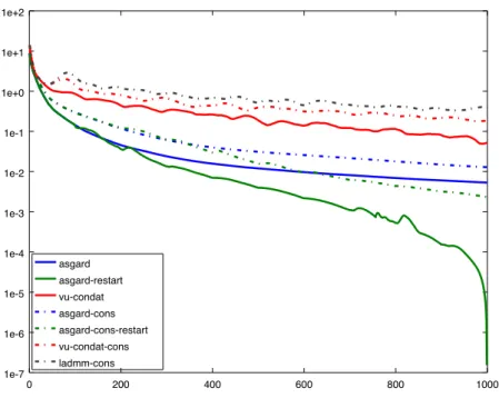
When the plot has dash-dotted line, we consider the constraint z = Dx and the augmented primal variable (x, z), otherwise, we directly split with h = k · k1. For ASGARD with restart, we
restart the momentum in the algorithm every 100 iterations; vu-condat is Vu-Condat’s algorithm and ladmm is the linearized ADMM method. For each algorithm we plot the difference between the current function value and the best function value encountered in the experiment (Figure1).
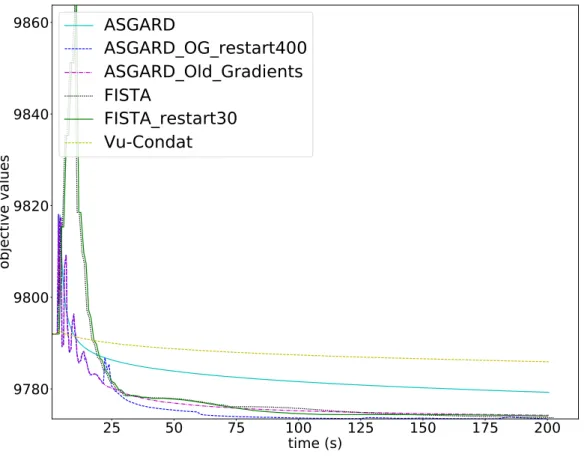
We also considered a medium-scale sparse and TV regularized problem on functional MRI data [12]. For given regularization parameters α > 0 and r ∈ [0,1], we would like to solve the following regression problem with regularization given by the sum of Total Variation (TV) and the`1 norm: min x∈Rn 1 2kAx−bk 2 2+α rkxk1+ (1−r)kM xk2,1 .
The problem takes place on a 3D image of the brains of size40×48×34. The optimization variable
xis a real vector with one entry in each voxel, that is n= 65280. MatrixM is the discretized 3D gradient. This is a sparse matrix of size 195840×65280 with 2 nonzero elements in each row. The matrixA ∈R768×65280 and the vectorb∈
R768correspond to 768 labeled experiments where each line ofAgathers brains activity for the corresponding experiment. Parameterr tunes the tradeoff between the two regularization terms. We choser = 0.1andα= 0.1.
In this scenario, we set the objective asf(x) = 12kAx−bk2
2,g(x) =αrkxk1 andh(y) = α(1− r)kyk2,1. On Figure2, we compared our algorithms against FISTA [3] with an inexact resolution of
0 200 400 600 800 1000 1e-7 1e-6 1e-5 1e-4 1e-3 1e-2 1e-1 1e+0 1e+1 1e+2 asgard asgard-restart vu-condat asgard-cons asgard-cons-restart vu-condat-cons ladmm-cons
Figure 1: Behavior of various algorithms for the synthetic sparse and TV regularized least squares problem: we plot the difference between the current function value and the best function value encountered vs iterations.
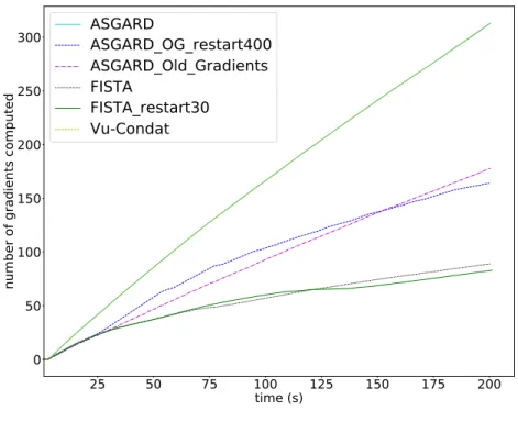
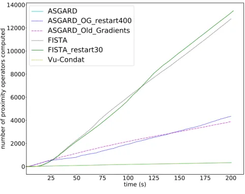
the proximal operator of TV, FISTA restarted every 30 iterations, and V˜u-Condat’s algorithm [14,6]. We can see that on this problem, ASGARD outperforms V˜u-Condat’s algorithm but not FISTA. After careful inspection, we realize that ASGARD (and also V˜u-Condat’s algorithm) spends too much time computing gradients off while FISTA spends much of its time to compute the proximity operator of g (Figures 3 and 4). Our framework allows us to consider useful variants in this setting. For instance, the use of old gradients makes ASGARD much faster in this problem in time. We can see on Figure2thatASGARD Old Gradientsoutperforms FISTA. Moreover, combined with a restart every 400 iterations, we obtain the best performance among the algorithms we test.
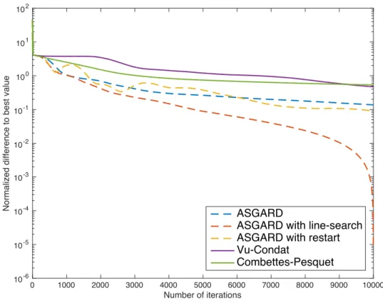
4.2 Quantum properties prediction
In materials science, quantum properties such as energy requires expensive calculations based on the density functional theory (DFT). Machine learning has been recently used to predict such properties for new molecules based on dataset derived by DFT. Let us represent the dataset by {(ri, pi)}Ni=1 whereri∈Rnis Coulomb matrix representation [11] ofi-th molecule andpi ∈Ris its properties. In this experiment, the Laplacian kernel, i.e.,K(r, r0) = exp(−kr−r0k1/σ)withk · k1is `1−norm ofRn, is used to measure the dissimilarity between molecules. A quantum property of a
25
50
75
100
125
150
175
200
time (s)
9780
9800
9820
9840
9860
objective values
ASGARD
ASGARD_OG_restart400
ASGARD_Old_Gradients
FISTA
FISTA_restart30
Vu-Condat
Figure 2: Comparison of various algorithms for the functional MRI problem: function value against computational time.
molecule with representationr is assumed to have the following form
e(r) =
N X
i=1
xiK(r, ri). (4.4)
The regression coefficients x = (x1, . . . , xN)T are obtained by solving the following elastic net
regularized minimization problem minimize x∈RN kKx−pk1+λ 2x TKx+ (1−λ)kxk 1, (4.5)
herep= (p1, . . . , pN)T andKij =K(ri, rj). Note that (4.5) is a particular case of (1.1) with
f(x) = λ 2x
TKx, g(x) = (1−λ)kxk
25
50
75
100
125
150
175
200
time (s)
0
50
100
150
200
250
300
number of gradients computed
ASGARD
ASGARD_OG_restart400
ASGARD_Old_Gradients
FISTA
FISTA_restart30
Vu-Condat
Figure 3: Comparison of various algorithms for the functional MRI problem: number of gradients evaluations against computational time.
In this case,
proxγg(x) = soft[−(1−λ)γ,(1−λ)γ](x) and proxγh∗(x) =x−γ p+ soft[−γ−1,γ−1](γ−1x−p)
. (4.7)
In Figure5, we compare the behavior of different versions of our ASGARD with Vu-Condat’s algo-rithm [6,14] and Combettes-Pesquet’s algorithm [4] on the dataset of 7211molecules in [11] in which50%molecules are used to train.[4].
5
Conclusion
In this paper, we build, based on the homotopy-based smoothing and acceleration technique of [ASGARD], a new method to solve a large class of generic convex optimization problems where the objective function is split into a sum of one smooth term and two non-smooth terms, one of which is combined with a linear operator. The variants of our method with line-search and old gradients benefits from the local smoothness of nonsmooth function and can avoid computing the whole gradient of the smooth function. In contrast to the existing methods in the literature, our method
25
50
75
100
125
150
175
200
time (s)
0
2000
4000
6000
8000
10000
12000
14000
number of proximity operators computed
ASGARD
ASGARD_OG_restart400
ASGARD_Old_Gradients
FISTA
FISTA_restart30
Vu-Condat
Figure 4: Comparison of various algorithms for the functional MRI problem: number of prox evaluations against computational time.
also features rigorous convergence guarantees. Numerical experiments with real-world problems illustrate the superiority of our method vs. the other state-of-the-art algorithms.
Acknowledgments.
The work of V. Cevher and Q. V. Nguyen is supported by the NCCR MARVEL, funded by the Swiss National Science Foundation. The work of O. Fercoq is supported by a public grant as part of the Investissement d’avenir project, reference ANR-11-LABX-0056-LMH, LabEx LMH and PGMO.
References
[1] Heinz H. Bauschke and Patrick L. Combettes.Convex analysis and monotone operator theory in
Hilbert spaces. CMS Books in Mathematics/Ouvrages de Math´ematiques de la SMC. Springer,
0 1000 2000 3000 4000 5000 6000 7000 8000 9000 10000 Number of iterations 10-6 10-5 10-4 10-3 10-2 10-1 100 101 102
Normalized difference to best value
ASGARD
ASGARD with line-search ASGARD with restart Vu-Condat
Combettes-Pesquet
Figure 5: Comparison with existing algorithms (σ= 4000andλ= 0.001).
[2] Amir Beck and Marc Teboulle. Fast gradient-based algorithms for constrained total vari-ation image denoising and deblurring problems. IEEE Transactions on Image Processing, 18(11):2419–2434, 2009.
[3] Amir Beck and Marc Teboulle. A fast iterative shrinkage-thresholding algorithm for linear inverse problems. SIAM J. Imaging Sci., 2(1):183–202, 2009.
[4] Patrick L. Combettes and Jean-Christophe Pesquet. Primal-dual splitting algorithm for solving inclusions with mixtures of composite, Lipschitzian, and parallel-sum type monotone opera-tors. Set-Valued Var. Anal., 20(2):307–330, 2012.
[5] Patrick L. Combettes and B˘ang C. V˜u. Variable metric forward-backward splitting with appli-cations to monotone inclusions in duality. Optimization, 63(9):1289–1318, 2014.
[6] Laurent Condat. A primal-dual splitting method for convex optimization involving Lips-chitzian, proximable and linear composite terms. J. Optim. Theory Appl., 158(2):460–479, 2013.
[7] Tom Goldstein, Brendan O’Donoghue, Simon Setzer, and Richard Baraniuk. Fast alternating direction optimization methods. SIAM Journal on Imaging Sciences, 7(3):1588–1623, 2014.
[8] Yura Malitsky and Thomas Pock. A first-order primal-dual algorithm with linesearch. arXiv
preprint arXiv:1608.08883, 2016.
[9] Yu. Nesterov. Smooth minimization of non-smooth functions. Math. Program., 103(1, Ser. A):127–152, 2005.
[10] Yu Nesterov. Universal gradient methods for convex optimization problems. Mathematical
Programming, 152(1-2):381–404, 2015.
[11] Matthias Rupp. Machine learning for quantum mechanics in a nutshell. International Journal
of Quantum Chemistry, 115(16):1058–1073, 2015.
[12] Sabrina M Tom, Craig R Fox, Christopher Trepel, and Russell A Poldrack. The neural basis of loss aversion in decision-making under risk. Science, 315(5811):515–518, 2007.
[13] Quoc Tran-Dinh, Olivier Fercoq, and Volkan Cevher. A smooth primal-dual optimization framework for nonsmooth composite convex minimization. arXiv preprint arXiv:1507.06243, 2015.
[14] B`˘ang Cˆong V˜u. A splitting algorithm for dual monotone inclusions involving cocoercive oper-ators. Adv. Comput. Math., 38(3):667–681, 2013.
[15] Yangyang Xu. Accelerated first-order primal-dual proximal methods for linearly constrained composite convex programming. To appear in SIAM Journal on Optimization, 2017.