Hyperbolic smoothing in nonsmooth optimization and applications

(1)

Hyperbolic smoothing in nonsmooth optimization

and applications

Alia Al Nuaimat

This thesis is submitted in total fulfilment of the

requirement for the degree of Doctor of Philosophy

School of Science, Information Technology and

Engineering, Faculty of Science,

Federation University Australia

PO Box 663

University Drive, Mount Helen

Ballarat, VIC 3353, Australia.

(2)

Abstract

Nonsmooth nonconvex optimization problems arise in many applications including economics, business and data mining. In these applications objective functions are not necessarily differentiable or convex. Many algorithms have been proposed over the past three decades to solve such problems. In spite of the significant growth in this field, the development of efficient algorithms for solving this kind of problem is still a challenging task.

The subgradient method is one of the simplest methods developed for solving these problems. Its convergence was proved only for convex objective functions. This method does not involve any subproblems, neither for finding search directions nor for computation of step lengths, which are fixed ahead of time. Bundle methods and their various modifications are among the most efficient methods for solving nonsmooth optimization problems. These methods involve a quadratic program-ming subproblem to find search directions. The size of the subproblem may increase significantly with the number of variables, which makes the bundle-type methods unsuitable for large scale non-smooth optimization problems. The implementation of bundle-type methods, which require the use of the quadratic programming solvers, is not as easy as the implementation of the subgradient meth-ods. Therefore it is beneficial to develop algorithms for nonsmooth nonconvex optimization which are easy to implement and more efficient than the subgradient methods.

In this thesis, we develop two new algorithms for solving nonsmooth nonconvex optimization problems based on the use of the hyperbolic smoothing technique and apply them to solve the pump-ing cost minimization problem in water distribution. Both algorithms use smoothpump-ing techniques. The first algorithm is designed for solving finite minimax problems. In order to apply the hyperbolic smoothing we reformulate the objective function in the minimax problem and study the relationship between the original minimax and reformulated problems. We also study the main properties of the hyperbolic smoothing function. Based on these results an algorithm for solving the finite minimax

(3)

problem is proposed and this algorithm is implemented in GAMS. We present preliminary results of numerical experiments with well-known nonsmooth optimization test problems. We also compare the proposed algorithm with the algorithm that uses the exponential smoothing function as well as with the algorithm based on nonlinear programming reformulation of the finite minimax problem.

The second nonsmooth optimization algorithm we developed was used to demonstrate how smooth optimization methods can be applied to solve general nonsmooth (nonconvex) optimization problems. In order to do so we compute subgradients from some neighborhood of the current point and define a system of linear inequalities using these subgradients. Search directions are computed by solving this system. This system is solved by reducing it to the minimization of the convex piecewise lin-ear function over the unit ball. Then the hyperbolic smoothing function is applied to approximate this minimization problem by a sequence of smooth problems which are solved by smooth optimiza-tion methods. Such an approach allows one to apply powerful smooth optimizaoptimiza-tion algorithms for solving nonsmooth optimization problems and extend smoothing techniques for solving general non-smooth nonconvex optimization problems. The convergence of the algorithm based on this approach is studied. The proposed algorithm was implemented in Fortran 95. Preliminary results of numerical experiments are reported and the proposed algorithm is compared with an other five nonsmooth opti-mization algorithms. We also implement the algorithm in GAMS and compare it with GAMS solvers using results of numerical experiments.

(4)

Statement of Authorship

Except where explicit reference is made in the text of the thesis, this professional thesis contains no material published elsewhere or extracted in whole or in part from a thesis by which I have qualified for or been awarded another degree or diploma. No other persons work has been relied upon or used without due acknowledgment in the main text and bibliography of the thesis.

(5)

Acknowledgement

First of all, I would like to acknowledge my great appreciation to my principal supervisor Associate Professor Adil Bagirov. It has been a great pleasure working with Associate Professor Bagirov over the years; learning from such a great Mathematician. I would like to thank him for accepting me as one of his students and for his great support during my PhD. His care, support, knowledge, availability and guidance was of inestimable value. The appreciation I have toward him is beyond words. The whole time I have spent as his student has definitely been a challenging and stimulating part of my life. Also, I would like to thank both my associate supervisors, Dr David Yost and Dr Andrew Barton, for their valued encouragement and ongoing advice with my research.

In addition to the invaluable support of all my supervisors, this PhD thesis would not have been possible without the financial support of the School of Science, Information Technology and Engi-neering (SITE). Then too, I would like to recognize Professor Sidney Morris, former head of Grad-uate School of Information Technology and Mathematical Science (GSITMS), for openly accepting me and financially supporting my studies, from the time of my arrival in Ballarat Australia. I also greatly appreciate the support and help from Dean of SITE, Professor John Yearwood, for allowing me study my PhD study in such encouraging and supportive environment.

As well as all the preceding, it would be remiss of me not to also acknowledge Associate Profes-sor Andrew Stranieri, the Director of Centre for Informatics and Applied Optimization (CIAO), for his direction and timely advice which was always so positive and encouraging. I also wish to sin-cerely thank Mr Frank Williams for his ongoing efforts and meticulous proof-reading of my research, thereby enriching the final outcome and quality of my thesis.

All of the persons highlighted herein have been most professional in their approach and each in their own special way has enhanced the quality of my research, plus the timely completion of my Doctoral thesis.

(6)

Dedication

(7)

List of publication

Journal papers

1. Bagirov, A.M., Al Nuiamat, A., and Sultanova, N., Hyperbolic smoothing function method for minimax problems,Optimization, 62(6), 2013, 759–782.

2. Bagirov, A. M., Jin, L., Karmitsa, N., Al Nuaimat, A., and Sultanova, N., Subgradient method for nonconvex nonsmooth optimization, Journal of Optimization Theory and Applications, 157(2), 2013, 416–435.

3. Bagirov, A. M., Barton, A. F., Mala-Jetmarova, H., Al Nuaimat, A., Ahmed, S. T., Sultanova, N., and Yearwood, J., An algorithm for minimization of pumping costs in water distribution systems using a novel approach to pump scheduling, Mathematical and Computer Modelling, 57(34), 2013, 873–886.

4. Bagirov, A. M., Ahmed, S. T., Barton, A. F., Mala-Jetmarova, H., Al Nuaimat, A., Sultanova, N. Comparison of metaheuristic algorithms for pump operation optimization.14th Water Dis-tribution Systems Analysis Conference, 2012.

5. Bagirov, A. M., Barton, A. F., Mala-Jetmarova, H., Al Nuaimat, A., Ahmed, S. T., Sultanova, N., and Yearwood, J., Minimization of pumping costs in water distribution systems using ex-plicit and imex-plicit pump scheduling,Hydrology and Water Resources Symposium, 2012. 6. Bagirov, A.M., Ozturk, G., Sultanova, N., and Al Nuaimat, A., Nonsmooth nonconvex

(8)

Conference and workshop presentations

1. Al Nuaimat, A., A Generalized Subgradient Algorithm for Unconstrained Nonsmooth, Non-convex Optimization,The 2011 IFORS conference in Nonsmooth Optimization III,

2. Al Nuaimat, A., An algorithm for minimization of pumping costs in water distribution sys-tems using a novel progressive approach for pump scheduling,The 9th EUROPT Workshop on Advances in Continuous OptimizationJuly, 2011.

(9)

List of Tables

(13)

List of Figures

2.1 Hyperbolic smoothing of the function (2.11). . . 30

3.1 Number of CONOPT iterations for unconstrained minimax problems. . . 59

3.2 Number of SNOPT iterations for unconstrained minimax problems. . . 59

3.3 Number of SNOPT function calls for unconstrained minimax problems. . . 60

3.4 Number of CONOPT iterations for general nonsmooth optimization problems. . . 60

3.5 Number of SNOPT iterations for general nonsmooth optimization problems. . . 61

3.6 Number of SNOPT function calls for general nonsmooth optimization problems. . . 61

4.1 Graph of test problem 2.3 (Spiral). . . 88

4.2 Number of function evaluations for unconstrained minimax problems. . . 88

4.3 Number of subgradient evaluations for unconstrained minimax problems. . . 89

4.4 Number of function evaluations for general nonsmooth problems. . . 89

4.5 Number of subgradient evaluations for general nonsmooth problems. . . 90

5.1 An example of a timeline. . . 98

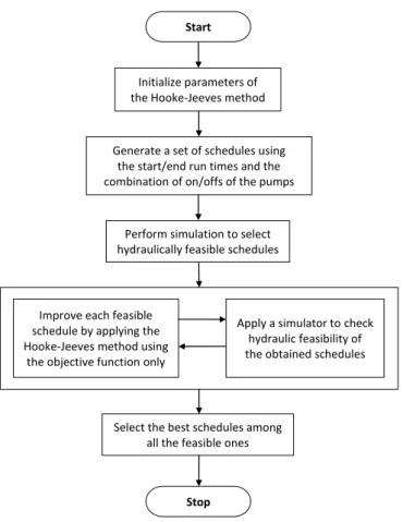
5.2 The algorithm for pumping cost minimization. . . 106

5.3 The water distribution system. . . 107

5.4 The optimal pump schedule. . . 107

5.5 Inflow and outflow from the network. . . 108

5.6 Time series water volume graphs for Tanks 1, 2 and 3. . . 109

(14)

Introduction

Optimization models are widely used in solving many practical problems including those in eco-nomics, operational research, mechanics and optimal control. In many applications optimization problems are nonsmooth, that is in these problems objective and/or constraint functions have dis-continuous gradients. Nonsmooth optimization problems are among most difficult in optimization. Over the last four decades a great deal of effort has been devoted to design algorithms for solving nonsmooth optimization problems. To date, problems of nonsmooth optimization have been mainly tackled by variants of the bundle methods[37,44,48,61,64,65,96], subgradient (including the space dila-tion) methods[88]and algorithms based on smoothing techniques[81].

The subgradient method is one of the simplest methods for solving nonsmooth optimization prob-lem. It was originally developed by N. Shor and then was modified by many authors (see[17,83,88] and more recent papers[1,13,67,68,69]). Its convergence was proved only for convex objective func-tions. The subgradient method uses one subgradient and one function evaluation at each iteration. It does not involve any subproblems neither for finding search directions nor for computation of step lengths. Moreover, step lengths are fixed ahead of time. Therefore, it is easy to implement this method. Although this method is very slow it is well known that some of its modifications might be more successful for solving large scale problems than other nonsmooth optimization methods. For example space dilation was proposed by Shor[88]to accelerate the direction finding towards the min-imum where a linear operator is constructed at each iteration to change the metric of the space (for more of these modifications see[68,69]). In general, subgradient methods have several important lim-itations ( e.g.lack of implementable stopping test, lack of decrease of the objective function at each iteration, possible poor rate of convergence, etc). Nevertheless, they are extremely popular among practitioners, because of their simplicity of implementation.

(15)

optimiza-tion. The fundamental idea of bundle methods is usually to approximate the subdifferential of the objective function by gathering subgradients from previous iterations in one bundle. By doing this, information about the local behavior of the objective function is obtained. The bundle methods are based on the use of convex models to the objective function and as a result it is efficient for minimiza-tion of convex funcminimiza-tions, however it is not always efficient for minimizaminimiza-tion of nonconvex funcminimiza-tions. These methods involve a quadratic programming subproblem to find search directions. The size of the subproblem may increase significantly as the number of variables increase which makes the bundle-type methods unsuitable for large scale nonsmooth optimization problems. Therefore most of the versions of the bundle method are not applicable for solving large scale nonsmooth optimization prob-lems (convex or nonconvex). Recently, the limited memory bundle method[46,45,40,41,42]_{has been}

proposed where aggregate subgradients and Quasi-Newton updates for sparse problems are combined to find search directions. At each iteration of this method only three subgradients with a certain type of the quasi- Newton updates are used to find search directions. The limited memory bundle method is a hybrid of the variable metric bundle methods and the limited memory variable metric methods. The method exploits simple aggregation of subgradients, and calculates the search direction using a limited memory approach. As a result, the time-consuming quadratic subproblem appearing in stan-dard bundle methods need not to be solved and the number of stored subgradients is independent of the dimension of the problem. The efficiency of this method has been proved by numerical results

[45]_.

The quasisecant method was introduced in[7]. Unlike bundle methods this method does not rely on the convex model of the objective functionf, instead it uses quasisecants which are overestimators of the objective function in some neighborhood of the current point. Results from[7]demonstrate that the quasisecant method is more efficient for solving nonconvex nonsmooth optimization problems than some versions of the bundle method. Moreover, results from[45] show that it is efficient for solving large scale problems. At the same time the quasisecant method requires more function and quasisecant (subgradient) evaluations than the bundle methods.

(16)

has been proposed to solve especially nonconvex optimization problems. Similar to the subgradient method, the SUNNOPT method does not contain any subproblem to find either descent direction or step length. A bundle of information of the objective function is used in some neighborhood of the iteration point and the direction finding procedure is very simple. Aggregation of only two subgra-dients or quasisecants are used in the search direction finding procedure. Versions of SUNNOPT using subgradients and quasisecants have been presented and numerical results are shown to prove its efficiency for both small and large scale problems.

Minimax problems arise in multiple disciplines including engineering design[89], control system design[21], economics[11], machine learning[4]. These problems are nonsmooth problems because of the presence of the ”max”. There are several different approaches to solve this problem (see, for example,[28,33]). Moreover, conventional nonsmooth optimization algorithms such as the bundle methods and its variations can also be applied to solve this problem[5,7,44,48,61]. Any Minimax prob-lem can also be reformulated as a nonlinear programming probprob-lem and therefore efficient nonlinear programming techniques can be applied to solve it. One of the methods to solve such problems is ap-plying a smoothing technique to replace the original nonsmooth problem by an approximate smooth one. Smoothing methods bring these problems close to continuously differentiable programming problems which can be solved by the conventional smooth optimization methods. The main feature of smoothing methods is to approximate the nonsmooth problems by a sequence of parameterized smooth continuously differentiable problems. Different smoothing techniques have been developed to replace the maximum function in minimax problem by a smooth function including the exponen-tial and hyperbolic smoothing functions. In[15]Ben-Tal and Teboulle introduce a general smoothing approach that utilizes recession functions to approximate a nondifferentiable optimization problem. It covers several types of problems including minimax problems using the so called recession function. The exponential smoothing function for the maximum functionf(x) = max

i=1,...,mfi(x)is as follows Fε(x) =εlog m X i=1 exp fi(x) ε (1)

(17)

whereεis called the precision parameter. The exponential smoothing function has been commonly used to construct many smoothing approximation algorithms for problems with min and max tions. Several smoothing methods are based on using exponential smoothing function (1). The func-tion (1) was first proposed in[50] within the structure of a penalty function method. The precision parameter in the exponential smoothing function may become extremely small too fast and cause ill-conditioning and floating-point overflow. In their paper[81]the authors made an effort to address this issue by introducing a feedback precision adjustment rule whereby the precision parameters are constructed by a subroutine. The goal is to ensure that the precision parameter remains large when away from the solution and is decreased when the solution is approached.

Another smoothing function is a hyperbolic smoothing function which is introduced for the func-tionmax{0, t}the first time in[97]:

φ(t, τ) = t+

√ t2₊_τ2

2 ,

whereτ >0is the precision parameter. In[98], the authors consider a problem of covering plane do-mains by circles which is modeled as a min-max-min problem which enables them to take advantage of the hyperbolic smoothing function to develop a minimization algorithm which solves a sequence of approximating problems. In the paper[99]this technique was applied to solve the cluster analysis problem using its nonsmooth optimization formulation.

Despite some applications hyperbolic smoothing functions have not been studied extensively so far. In this thesis we study this smoothing technique in detail. In order to apply the hyperbolic smoothing to the finite maximum functions these functions are represented as a sum of the maximum of two functions by adding a new variable. We study the relationship between the set of stationary points of the latter function and that of the original maximum function. The new function is ap-proximated using hyperbolic smoothing functions and differential properties of the approximating function are studied. It is demonstrated that smooth optimization solvers can be applied to minimize the approximating function. We design an algorithm for solving minmax problems using the

(18)

hyper-bolic smoothing. Furthermore, we present results of numerical experiments using two solvers from GAMS: CONOPT and SNOPT. We also compare these results with those obtained using exponential smoothing and also nonlinear programming reformulations of minimax problems. Such an approach allows one to solve the finite minimax problem using existing powerful smooth optimization solvers. The smooth function approximates the objective function and this approximation is controlled by the precision parameter(s).

Next we extend this method for solving general nonsmooth nonconvex optimization problems. In this approach the problem of finding search directions is reduced to the minimization of a con-vex piecewise linear function over the unit ball. The hyperbolic smoothing functions are applied to approximate the convex piecewise linear function by a smooth function which is minimized to find search directions. We present convergence results for the proposed algorithm. The algorithm is im-plemented in Fortran 95. Results of numerical experiments are reported and the proposed algorithm is compared with another five nonsmooth optimization algorithms. We also implement the algorithm in GAMS and compare it with GAMS solvers using results of numerical experiments.

The proposed methods is applied to solve Pump scheduling problem in water distribution system.

Outline of the Thesis

This thesis is organized into six chapters beginning with a background discussion in Chapter 1 which introduces the reader to nonsmooth optimization fields from nonsmooth optimization analy-sis to nonsmooth optimization theory. Chapter 2 presents an overview of nonsmooth optimization methods and Chapter 3 describes the application of the hyperbolic smoothing to the finite maximum functions. Then, Chapter 4 provides a description for solving general nonsmooth nonconvex prob-lems. Chapter 5 describes the minimization of pumping costs in water distribution systems. Whilst, Chapter 6 concludes the thesis and gives recommendations for future research directions.

(19)

Chapter 1

Background

The chapter is organized as follows. First we introduce basic notations and definitions that will be used throughout the rest of this thesis, followed by basic definitions and results of Nonsmooth Analysis and Optimization. We also present some properties of the subgradients and subdifferentials for convex function. Following that, we give the extension of these concept to a nonconvex case. Finally, we give the necessary optimality conditions and linearizations for locally Lipschitz functions.

1.1 Notations and Definitions

IRnis then-dimensional real Euclidean space, we denote byx= (x1, . . . , xn)a point inIRn, and

we denote byhx, yi :=

n

P

i=1

xiyi an inner product of the two pointsx, y ∈IRn, andk · kdenotes the

associated Euclidean norm.

S1 :={x∈IRn:kxk= 1}is the unit sphere, whereasBε(x) :={y∈IRn:ky−xk< ε}is the

open ball centered atxwith the radiusε >0. Furthermore, an open ball with radiusε >0centered at0is denoted byBε:=Bε(0n).

A setS ⊂IRnis called convex ifλx+ (1−λ)y ∈S for anyx, y∈ Sandλ∈ [0,1]. A linear combinationPk

i=1λixiis called a convex combination of pointsx1, ..., xk∈IRnif eachλi≥0and

Pk

i=1λi = 1. Theconvex hullof a setS, denoted by conv S, is the smallest convex set containingS.

A functionf : IRn→IRis convex function if

(20)

for allx, y∈IRnandλ∈[0,1].

A functionf : IRn → IRis said to be Locally Lipschitz at ( or near) the pointxif there exist a numbersδ, L >0such that

|f(y)−f(z)| ≤Lkf(y)−f(z)k

for ally, z ∈Bδ(x).

1.2 Nonsmooth Analysis

The theory of Nonsmooth analysis was first developed for convex functions. Here we first go over a number of definitions and results for convex analysis. Second, define the subgradient and also the subdifferential of the convex function, and then finally we generalize these results to nonconvex locally Lipschitz functions.

Definition 1. The directional derivativef0(x, d)of the functionf:IRn→IRatxin the direction of

d∈IRnis defined as

f0(x;d) = lim

t↓0

f(x+td)−f(x)

t

Definition 2. A function f : IRn → IR is called upper semicontinuous at x ∈ IRn if for every

sequence{xk}converging tox

lim sup

k→∞

f(xk)≤f(x),

and is called lower semicontinuous if

f(x)≤lim inf

k→∞f(xk),

Definition 3. The subdifferential of a convex functionf : IRn→IRatx∈IRnis the set

∂cf(x) ={g∈IRn|f(y)≥f(x) +hg, y−xi, ∀y ∈IRn}

(21)

For any differentiable function ,∂cf(x) ={∇f(x)}.

Definition 4. Letε >0. Theε-subdifferential of the convex functionf : IRn→IRis the set

∂εf(x) :={g∈IRn|f0(x)≥f(x) +hg, x0−xi −ε, ∀x0∈IRn}

each elementξ ∈∂εf(x)is called anε-subgradient of the convex functionf atx.

Theorem 1(Rademacher). [25]LetSbe an open set. A functionf :S →IRthat is locally Lipschitz continuous onSis differentiable almost everywhere onS.

The next theorem presents the relationship between subdifferential and the directional derivative.

Theorem 2. Letf : IRn→IRbe convex function atx∈Rn_{. Then for all}_x_∈_Rn

(i) ∂f(x)is a nonempty, convex, and compact set such that∂f(x)⊆BL(0),

(ii) ∂cf(x) ={g∈Rn:f0(x, d)≥ hg, di}, ∀d∈Rn,

(iii) f0(x, d) = max

g∈∂cf(x)

{hg, di}, ∀d∈Rn,

whereLis a Lipschitz constant off.

The classical directional derivative and subdifferential, in general, do not exist for locally Lips-chitz function. F. Clarke introduced the generalizations of directional derivatives and subdifferentials for locally Lipschitz functions[25].

Definition 5. The generalized directional derivative f0(x, d) of the locally Lipschitz function f : IRn→IRatx∈Rnin the directiond∈IRnis defined as

f◦(x;d) = lim sup

y→x t↓0

f(y+td)−f(y)

t .

Definition 6. (Clarke subdifferential)[25] The subdifferential∂f(x) of a locally Lipschitz function

f : IRn→IRat a pointx∈IRnis given by

(22)

Hereg∈∂f(x)is called a subgradient off atx.

According to Rademacher theorem locally Lipschitz functions are differentiable almost every-where and their subdifferential can also be defined as follows:

∂f(x) =conv lim i→∞∇f(xi)| xi→xand ∇f(xi)exists .

Definition 7. A locally Lipschitz functionf : IRn → IRis called regular atxiff it is directionally

differentiable atxand

f0(x, d) =f0(x, d), ∀d∈IRn.

The following theorem summarizes some properties of the Clarke subdifferential.

Theorem 3. [61]Letf : IRn→IRbe locally Lipschitz function atx∈Rnwith constantK. Then

(i) ∂f(x)is nonempty, convex, compact set such that∂f(x)⊆BK(0),

(ii) f◦(x;v) = max{hξ, vi|ξ∈∂f(x), ∀x∈IRn},

(iii) the mapping∂f(·)is upper semi-continuous.

Note that, for convex function the Clarke subdifferential coincides with the subdifferential from Definition (3). This means that the Clarke subdiiferential is the generalization of the subdifferential for convex functions. Furthermore, for any locally Lipschitz functionf, we have∇f(x)∈∂f(x).

TheGoldsteinε-subdifferential for locally Lipschitz functions is defined as follows.

Definition 8. Letf : IRn→ IRbe a locally Lipschitz function atx ∈Rnε >0, then the Goldstein

ε-subdifferential of the Lipschitz functionf : IRn→IRis the set

∂_εGf(x) :=conv{∂f(y)|y∈B¯ε(x)}

(23)

1.3 Nonsmooth Optimization Theory

In this section, we present basic results from nonsmooth optimization including necessary and sufficient conditions for a minimum. Moreover, linearization of local Lipschitz functions using sub-gradients will be discussed.

We consider the following unconstrained optimization problem:

minimize f(x) subject to x∈IRn, (1.1)

where the objective functionf : IRn→IRis assumed to be locally Lipschitz.

Definition 9. A pointx? ∈ IRn is called a global minimum off if it satisfiesf(x?) ≤ f(x)for all

x∈Rn.

Definition 10. A point x? ∈ IRn is called a local minimum of f if there exists > 0 such that

f(x?₎_≤_f₍_x₎_{for all}_x_∈_B (x?).

Theorem 4. Letf: IRn→IRbe a locally Lipschitz atx?∈IRnand attains its local minimum atx?.

Then

(i) 0∈∂f(x?)and

(ii) 0∈∂_εGf(x?),

(iii) f◦(x?, d)≥0, ∀d∈IRn.

The pointx∗ ∈IRnis called stationary iff0∈ ∂f(x∗). Stationarity is a necessary condition for local optimality and, in the convex case, it is also sufficient for global optimality.

In order to develop nonsmooth optimization algorithms for unconstrained optimization problem (1.1), linearization of the objective function needs to be built. Using these linearizations we are able to construct a piecewise linear local approximation to the unconstrained optimization problem.

(24)

Definition 11. Letf : IRn→IRbe a locally Lipschitz function atxand letξ∈∂f(x)be an arbitrary

subgradient. Then theξ-linearization offatxis the functionf¯ξ : IRn→IRdefined by

¯

fξ(y) :=f(x) +hξ, y−xi, ∀y∈IRn

and the linearization off atxis the functionfˆx:IRn→IRsuch that

ˆ

fx(y) := max{f¯ξ(y)|ξ ∈∂f(x)}, ∀y∈IRn.

Some basic properties of the linearizationfˆxare presented in the following theorem.

Theorem 5. Letf:IRn→IRbe locally Lipschitz atx. Then the linearizationfˆxis convex and

(i) fˆx(x) =f(x),

(ii) fˆx(y) =f(x) +f◦(x;y−x), ∀y∈IRn,

(iii) ∂fˆx(x) =∂f(x).

Finding descent direction for a locally Lipschitz function is an important step of any optimization algorithm. We first give the general definition of a descent direction for any function, then modify it using generalized directional derivatives and subdifferential.

Definition 12. The directiond∈ IRnis called a descent direction for the functionf : IRn → IRat

x∈IRnif there existsε >0such thatf(x+td)< f(x), ∀ t∈(0, ε].

Theorem 6. Letf : IRn →IRbe locally Lipschitz atx, the directiond∈IRnis a descent direction

forf atxif any of the following holds: (i) f◦(x;d)<0,

(25)

(iii) hξ, di<0, ∀ξ ∈∂_εGf(x),

(26)

Chapter 2

Nonsmooth Optimization Methods

We consider the following unconstrained minimization problem:

minimize f(x) subject to x∈IRn, (2.1)

where the objective functionf : IRn→IRis assumed to be locally Lipschitz and this function is not necessarily either differentiable or convex.

Numerous algorithms have been developed for solving problem (2.1), with similar basic structure. Their main point of difference is based on the specification of search directions and the selection of step size. The general structure of an iterative algorithm for solving the nonsmooth optimization problem (2.1) can be described as follows.

Step 1. Initialization Step: Choose a starting pointx1∈Rn. Set the iteration counter to i:=1.

Step 2. Stopping criterion: If the optimality condition atxiis satisfied then stop. Otherwise, go to step

3.

Step 3. Direction finding: Find a search directiondiusing either the subgradientgi ∈∂f(xi)or some

approximation to the subdifferential∂f(xi).

Step 4. Line search: Select an appropriate step sizeλi >0, and computexi+1 =xi+λidi. Increase i

by 1, and go to step 2.

The desirable choices of the directiondi, and the step sizeλi, have been the principal points of

(27)

to solve nonsmooth optimization problems: deterministic methods and stochastic methods. Deter-ministic optimization algorithms guarantee under some assumptions that, starting from a given initial point, an algorithm converges with deterministic steps in a finite number of iterations. On the other hand, stochastic methods cannot adopt the same methodology. Stochastic methods are not guaranteed to achieve the same solution in any single run. Deterministic algorithms have often been shown to be better than stochastic ones at solving large scale nonsmooth nonconvex problems at a consider-able computational cost and quality of the solution[53]. In this thesis, we will focus on Deterministic optimization methods. The most popular deterministic optimization algorithms are accordingly di-vided into three main classes; subgradient methods, bundle methods and methods based on smoothing techniques. In this chapter we will review some of these algorithms.

2.1 Subgradient methods

The subgradient method was originally developed by N. Shor in the mid 1960s and then modified by many authors (see[17,83,88]and more recent papers[1,13,67,68,69]).

It generalizes the steepest descent method of smooth optimization by replacing the gradient by an arbitrary subgradient. The subgradient method uses one subgradient and one function evaluation at each iteration. It does not involve any subproblems either for finding search directions or for computation of step lengths. Therefore, it is easy to implement. In addition it can be immediately applied to a far wider variety of problems. The memory requirement of subgradient methods can be much smaller than the bundle type methods, which means it can be used for extremely large problems for which bundle type methods cannot be used. Although the subgradient method is very slow it is well known that some of its modifications might be more successful for solving large scale problems than other nonsmooth optimization methods[68,69]. The convergence of the subgradient method was proved only for convex problems.

(28)

descent method which takes the ant-gradient direction with fixed step size.

dk=−∇f(xk) (2.2)

where∇f(xk)is the gradient at the current iteration point.

The steepest descent method is one of the simplest optimization methods, though easy to imple-ment, however, this method has the disadvantage of the large number of zigzag moves[55]. As a result, the conjugate gradient method has been developed, which is more efficient where gradients at pre-vious iteration points are taken into account to compute the descent search direction. The conjugate gradient method has improved convergence rate the steepest descent method.

In the nonsmooth case of Problem (2.1), the gradient may not always exist at x. We assume that the objective function f is a locally Liptchitz function, where at least one subgradient can be calculated at any given point x, which is a mild assumption about most nonsmooth optimization problems.

The subgradient method is a generalization of steepest descent method (2.2) for smooth optimiza-tion problems. The idea of the subgradient method is quite simple by replacing the gradient∇f(xk)

by an arbitrary subgradientξk∈∂f(xk). Ifxkis not a stationary point thenξk6= 0and we compute

the search direction by normalizing the subgradientξk:

dk=−ξk/kξkk. (2.3)

Then the subgradient algorithm can be constructed as follows

Algorithm 1. Subgradient algorithm

Step 1. Choose a starting pointx1 ∈IRn. Set k:=1

Step 2. Givenxk, calculatef(xk), and an arbitrary subgradientξk∈∂f(xk). If the stopping criterion

is satisfied, then stop. Step 3. computedk=−ξk/kξkk.

(29)

Step 4. Select an appropriate step lengthλk>0.

Step 5. Setxk+1:=xk+λkdk, putk:=k+ 1and go to step 2.

There are some requirements for the step sizeλk to guarantee the global convergence. The step

lengthλkshould be defined so that to satisfy the following conditions:

1. The constant step sizeλkis chosen as a sufficiently small.

2. The step sizeλksatisfies the following condition:

λk>0,

∞ X

k=0

λk=∞.

The convergence of subgradient methods is proved for only convex problems. To our best knowl-edge such proof does not exist for nonconvex nonsmooth functions. Moreover, the subgradient method does not guarantee the decrease of the objective at each iteration. In addition, subgradi-ent method does not have practical termination criteria other than a maximum limit on the number of iterations. Poor performance of subgradient methods can happen when the direction is almost orthog-onal to a direction pointing toward a minimum. Because of these difficulties with the choice of the step length, there have been many attempts to improve the search and step length[12,38,82,88]. The space dilation methods were introduced[88], which can be considered as a nondifferentiable version of Quasi-Newton methods. These methods are based on accommodating previous iteration informa-tion. Similar to the use of the Hessian matrix or its approximation in quasi-Newton approaches, a suitable matrix is generated to multiply the subgradient in order to deflect the direction toward an optimal direction. One approach uses space dilation along the gradient, another approach uses space dilation along the difference of the two successive subgradients.

2.2 Cutting plane methods

Cutting-plane methods were proposed by Cheney and Goldstein [23] as well as by Kelley [47]. The cutting plane methods rely on construction of the lower approximation (underestimation) of the

(30)

objective function. This approximation is used to find the minimum of the original function. They are based on minimization of piecewise-affine approximation of the objective function, in which a new direction is obtained from the set of the previous subgradients, as opposed to using only one subgradient at a time, without a memory of past iterations on subgradient methods. The idea behind cutting plane methods is to approximatefusing a piecewise linear function, in other words, to replace f by a so-called cutting plane model. At the current iterationk, the piecewise linear approximation of the objective functionf can be defined as follows

ˆ

fk(x) :=max{f(xj) +hξj, x−xji|j∈Jk}, x∈IRn

whereξj is the subgradient at the trial pointsxj around the current pointxk,fˆk(x)is an

underesti-mator for convex functionf andJkis a set of subgradients calculated so far. Note that the idea of the

Cutting plane is to replace the original functionf by its approximationfˆk(x). The next iterate is then defined where the search directiondkis calculated by solving the following minimization problem:

minfˆk(xk+d)−f(xk) subject to d∈IRn (2.4)

which can be modified to the following linear problem.

min υ

st. υ≥f(xj) +hξj, x−xji, j∈Jk,

The cutting plane method does not always have a solution and is not used in practice due to poor convergence results. Furthermore, Cutting plane method can be very slow when new iterates move too far away from the previous ones. In order to improve the rate of convergence we can obtain the search direction by solving the following local subproblem

(31)

min υ+ 1 2kdk

2 _(2.5)

st. υ≥ −αk_j +ξ_jTd for allj ∈Jk,

where the regularizing quadratic penalty term is added to guarantee the existence of the solutiondk

and to keep the approximation local enough, where the search direction can obtain as follows

dk=−

X

j∈Jk

λk_jξj

It is easy to see that the search direction at xk is obtained as a convex combination of some

subgradients at the pointsyj, whereλk_j is the solution of the dual problem.

The main steps of the Cutting plane algorithm are as follows.

Algorithm 2. (Cutting plane algorithm)

Step 1.letδ >0a given stopping tolerance,S 6=∅be a compact convex set containing a minimum point off, choose any starting pointx1 ∈S, and setk:= 1.

Step 2.If

kf(xk)−fˆk−1(xk)k< δ,

then stop.

Step 3.Compute the search directiondkatx=xkas a solution of problem (2.5).

Step 4.Taketk= 1constant step size, and setxk+1:=xk+dk, Setk:=k+ 1and go to Step 2.

2.3 Bundle methods

Basically, subgradient methods use only one subgradient at each iteration, without a memory of past information iterations. If, instead, the past information obtained so far is kept, it is possible to

(32)

define piecewise-affine approximation of the objective function. The bundle method uses piecewise affine approximations to find search directions. These methods are among most efficient in nonsmooth optimization. In what follows we give a review regarding the bundle algorithms.

2.3.1 Standard bundle method

The bundle method was first introduced by C. Lemar´echal in [52] and then modified by many authors[5,7,35,36,43,48,61,65]. The basic idea of bundle methods is to approximate the subdifferential of the objective function by gathering subgradients from previous iterations into a bundle, which can be used to describe the local behavior of the objective function, as opposed to using only the current subgradients (like in the subgradient method). This subgradient information serves for the construction of a piecewise linear local approximation to the objective function. A search direction for this approximation is usually obtained as a solution of quadratic programming subproblem[61]. The global convergence of bundle methods with a bounded number of stored subgradients can be guaranteed[48].

The basic idea of bundle type algorithms consists of replacing the subdifferential by some poly-tope approximation. Indeed, if the approximation is sufficiently good the algorithm will find a descent direction and a new pointxk+1will decrease the value of the objective function. In case the

approxi-mation is bad we stay atxkand try to improve the approximation by adding further subgradients.

Consider the nonsmooth unconstrained minimization problem (2.1). Bundle method produces a sequence of pointsxk ⊂ IRn that converges to a global minimum of a convex function f or a

stationary point of the nonconvex functionf. First, we define the Cutting plane model functionfˆ(x)

that approximates the objective function at the iteration pointxkby

ˆ

fk(x) := max

j∈Jk

f(yk) +hξj, x−yki −αkj, j∈Jk⊂ {1, ..., k},

(33)

Hereξj ∈ ∂f(yj) is the subgradient of the trial point yj ∈ IRn from previous iteration, and Jk

nonempty index set,α_jkis calledlinearization errorwhich measures how good the model of the orig-inal problem is. For a convex functionf the linearization errorαk_j is nonnegative, but for nonconvex case it can be negative. Therefore, the linearization error for nonconvex functions was replaced by the subgradient locality measureβ_jk

β_jk=max{|αk_j|, γ(xk−yj)ω},

hereγ > 0is called a distance measure parameter,ω ≥ 1is called a locality measure parameter. The next iteration is obtained as

yk+1 :=xk+dk,

where the search directiondkis calculated as

dk:=arg min d∈Rn ˆ fk(xk+d) + 1 2hd, Dkdi , (2.6)

whereDkis symmetric, positive definiten×nmatrix that accumulates information about the

curva-ture of the objective functionf in a ball around the pointxk[62]. The role of the stabilization term

1

2hd, Dkdiis to keep the approximationfˆkof the objective functionf local enough.

A serious step is taken

xk+1 =yk+1 (2.7)

and Jk+1 =Jk∪ {k+ 1} for allj∈Jk,

iff(yk+1)is significantly less thanf(xk), otherwise, a null step is taken

xk+1 =xk (2.8)

(34)

By updating the index setJkwe improve the Cutting plane modelfˆk+1in both steps. Notice that

the quadratic direction finding minimization problem (2.6) can be rewritten as follows

min ν+1

2hd, Dkdi (2.9)

st. −β_jk+hd, ξji ≤ν for allj∈Jk,

The solutiondkof problem (2.9) can be found by solving quadratic dual problem as follows

dk =−

X

j∈Jk

λk_jDk−1ξj

whereP

j∈Jkλj = 1andλj ≥0, for allj ∈Jk.

Bundle methods have been developed for solving problem (2.1), with similar basic structure. Their main point of difference is based on the choice of the Cutting plane approximationfˆk, the

linearization errorβk_j and stabilizing matrixDk[62].

Algorithm 3. (Standard Bundle algorithm)

Step 1. (Initialization) Choose the stopping toleranceδ , line search parameterε, distance measure parameterγ > 0. Choose any starting pointx1 ∈ IRn, positive definite matrix D1, sety1 = x1,

J1={1}. Set the iteration counterk:= 1.

Step 2.(Direction finding) Solve the quadratic dual problem of problem (2.9) to find the directiondk

and the minimal value$kof problem (2.9).

Step 3.(Stopping criterion) If

$k < δ,

then stop withxkthe final solution.

Step 4.(Line search) Determine the step sizetkby a line search algorithm. If

(35)

do Serious step

xk+1 :=xk+tkdk

otherwise do Null step

xk+1 :=xk

Step 5. (updating) Determine the stabilization matrixDk+1 using an updating formula. Determine the index setJk+1and go to Step 2.

The convergence of bundle methods can be proved under some assumptions[48]. The computa-tional results show that the bundle methods perform significantly better than the subgradient method for minimizing nonsmooth convex functions. However, a solution to quadratic Problem (2.9) is time consuming for large scale nonsmooth optimization problems. Several types of bundle methods have been developed to avoid such costly computation. Variable metric bundle type methods are the most powerful method among them, where the time cosuming quadratic Problem (2.9) does not need to be solved.

Bundle methods need relatively large bundles to solve the problems efficiently. In other words, the size of the bundle has to be approximately the same as the number of variables[48]

2.3.2 Variable metric bundle type methods

The variable metric method for convex unconstrained minimization was proposed in[56]. Since this method is relatively robust and efficient even in the nonsmooth case, it has been extended for convex nonsmooth unconstrained minimization in[94]. Variable metric bundle methods are hybrid methods of the standard variable metric method and standard bundle method. The idea of the method is to use only three subgradients for direction determination; one at the current pointxk, the other at a

trial pointyk+1, and the last aggregated one containing information from past iterations. This means

that the dimension of quadratic programming subproblem is only three. Therefore, the size of the bundle does not need to grow with the dimension of the problem. To ensure the global convergence, the matrices are chosen to be uniformly positive definite. However, these methods use dense

(36)

ap-proximations of the Hessian matrix to calculate the search direction which become inefficient when the dimension of the problem increases. Practical optimization problems often involve nonsmooth functions of hundreds of variables; which can be a dilemma.

2.3.3 Limited memory bundle methods

For large scale nonsmooth optimization problems, it can be time consuming to use the variable metric bundle methods. Thus, a hybrid method of a variable metric bundle methods[57,94] and a limited memory variable metric methods[20,74]has been proposed[40,41,42]. In this method the ap-proximation of the Hessian matrix updates uses the information of the last few iterations to define a variable metric approximation. In practice, this means that the approximation of the Hessian matrix is not as accurate as that of the original variable metric bundle methods but both the storage space required and the number of operations used are significantly smaller. The Limited memory bundle method efficiency has been proved by numerical results. At each iteration of this method only three subgradients with a certain type of the quasi Newton updates are used to find search directions. The method exploits simple aggregation of subgradients, and calculates the search direction using a lim-ited memory approach. As a result, the time consuming quadratic subproblem appearing in standard bundle methods need not be solved and the number of stored subgradients is independent of the di-mension of the problem. SR1update andBF GS update of the matrix in descent direction finding are used individually for a null step and a serious step to guarantee the convergence of the algorithm.

2.3.4 Quasisecant method

In bundle methods, the subdifferential of the objective function is approximated using those sub-gradients that provide good underestimators from previous iterations. For convex functions, it is easy to find relevant subgradients from the previous iterations. However for nonconvex functions subgradi-ent information produces only local approximation to the objective function and should be discounted when no longer relevant. Unlike the convex case, in the nonconvex case, in general, not all subgra-dients provide a tight local approximation to a function. Therefore, subgrasubgra-dients which provide such

(37)

an approximation of a function in some neighborhood of a point are of big interest. To address this problem (at least partially) the notion of the quasisecant was introduced in[7]. quasisecants will be explained in greater detail in section (4.1). It was demonstrated that quasisecants can be efficiently computed for some nonsmooth functions. These include convex functions, functions represented as a maximum of a finite number of smooth functions, functions represented as a difference of two convex (DC) functions. Some interesting functions such as functions represented as a maxima of minima of a finite number of smooth convex functions (which includes continuous nonconvex piecewise linear functions), functions represented as a sum of minima of a finite number of smooth convex functions can be easily represented as a difference of two (nonsmooth) convex functions. Quasisecants are approximate subgradients. Quasisecant provide overestimation for the objective function in some neighborhood with a point. The computational results of the quasisecant method for solving well known nonsmooth optimization show that the bundle method performs significantly better than the quasisecant method for convex functions whereas the quasisecant method outperforms the bundle method for nonconvex nonregular problems.

2.4 Methods based on smoothing techniques

Consider the minimization problem

minimizef(x)subject to x∈IRn (2.10)

where

f(x) = max

i∈I fi(x), I ={1, . . . , m}, (2.11)

and the functionsfi, i∈I are continuously differentiable.

These problems are nonsmooth problems because of the presence of the ”max” operator and ap-pears in many application , such as vehicle routing (see, for example,[2,3]), location (see, for exam-ple,[16,32]), resource-allocation (see, for example,[60,78]), structural optimization (see, for example,

(38)

[10,24]_{) and many more.}

There exist many algorithms for solving Problem (2.10) (see, for example, [28,33]). Moreover, conventional nonsmooth optimization algorithms such as the bundle methods and its variations can also be applied to solve this problem [5,7,44,48,61]. Problem (2.10) can also be reformulated as a nonlinear programming problem and therefore efficient nonlinear programming techniques can be applied to solve it.

One of the methods to solve nonsmooth optimization problems is applying a smoothing tech-nique to replace the original nondifferentiable problem by an approximate smooth one. Smoothing techniques bring these problems close to continuously differentiable equations or continuously differ-entiable programming problems which can be solved by the conventional smooth optimization meth-ods. It has been shown that the smoothing approximation techniques are efficient methods for solving certain specially structured nonsmooth problems. Many of the algorithms are based on reformulat-ing the problem. Smoothreformulat-ing methods have been developed for solvreformulat-ing many important optimization problems including min-max problems. The main feature of smoothing methods is to approximate the nonsmooth nondifferentiable problems by a sequence of parameterized smooth continuously dif-ferentiable problems, and to trace the smooth path which leads to solutions. The accuracy of the approximation is controlled by some parameter, which is called a smoothing or precision parameter. In the last decade many smooth approximation functions have been developed. A smooth approxi-mation of the ”max” function simplifies the problem and facilitates a platform for us to study related problems.

Recently, different smoothing techniques have been developed to replace the objective function f in Problem (2.10) by a smooth function. Such an approach allows one to solve the finite minimax problem using smooth optimization solvers. The smooth function approximates the objective function f and this approximation is controlled by the precision parameter(s). We can divide smoothing tech-niques into two main classes. Smoothing techtech-niques from the first class try to smooth the objective function only in some neighborhood of the so-called kink points (points where the functionf is not differentiable) whereas smoothing techniques from the second class smooth the objective functionf

(39)

globally.

The paper[103]introduces different functions to smooth the finite maximum function at the kink points. In the paper[34], the authors reformulate the finite minimax problem replacing the maximum function by the sum of more simple maximum functions and develop smooth approximations of the reformulated function. This smooth function approximates the reformulated function only at the points where the function is not differentiable.

Smoothing techniques from the second class include the exponential and hyperbolic smoothing functions. The general approach for smoothing was introduced in [15] where different smoothing functions, including exponential smoothing function, were considered. The paper[93] considers the logarithmic barrier function of the epigraph of the maximum function to smooth it. In the paper[102]_,

the author introduces a smoothing method for minimax problems based on the exponential smoothing function. He proves its convergence and provides results of preliminary numerical experiments. The paper[81]introduces another version of smoothing technique using exponential smoothing. A feed-back precision-adjustment rule is used to update the precision parameter in the exponential smoothing function which allows to avoid the ill-conditioning associated with large precision parameters.

In the paper[100], a truncated exponential smoothing function is introduced which is later com-bined with a Newton-Armijo algorithm to solve a minimax problem. A generalization of the expo-nential smoothing algorithm for finite min-max-min problems was considered in[90]. A smoothing technique is applied twice, once to eliminate the inner min operator and once more to eliminate the max operator.

2.4.1 Exponential penalty smoothing method

Ben-Tal and Teboulle[15], introduced a smoothing technique for nondifferentiable optimization problems with maximum objective functions. The tool they used to generate such an approximate problem is through the use of the recession approximate problem by a smooth optimization problem which contains a smoothing parameter. This parameter controls the accuracy of the approximation. This smoothing approach has also been proposed and used to smooth min-max problems by Polak

(40)

[81]_{. This method is called exponential smoothing function.}

Consider

Ψ(x) = max

i=1,...,mfi(x), i= 1, ..., m,

where the functionsfi, i= 1, ..., mare continuously differentiable.

Letµ >0be a smoothing parameter. Define the following function[81]

Ψµ(x) = 1 µlog m X i=1 expµfi(x)_. _(2.12)

It follows from (2.12) that

1. Ψ(x)≤Ψµ(x)≤Ψ(x) +1_µlogm.

2. Ψµ(x)is decreasing with respect toµ.

3. Ψµ(x)→Ψ(x)asµ→+∞.

4. Ψµ(x)is twice continuously differentiable for allµ >0.

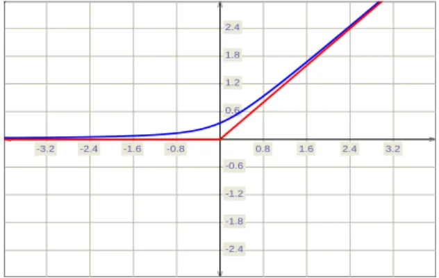
2.4.2 Hyperbolic smoothing functions

The paper[97]was the first instance where the hyperbolic smoothing function was considered. In the paper[98], the problem of the optimal covering of plane domains by circles was solved by applying a hyperbolic smoothing technique and in the paper[99]this technique was applied to solve the cluster analysis problem using its nonsmooth optimization formulation.

The hyperbolic function was introduced for the following function:

f(x) = max{0, x}. (2.13)

The hyperbolic smoothing of this function is as follows:

φτ(x) =

x+√x2₊_τ2

(41)

whereτ >0is a precision parameter.

Proposition 1. The functionφτ(x)has the following properties:

1. φτ(·)is an increasing convexC∞function;

2. f(x)< φτ(x)≤f(x) +

τ

2, ∀x∈IR.

Proof. The proof is straightforward.

The hyperbolic function for smoothing the function (2.13) is illustrated in Figure (2.1) where blue curve shows the smoothing function.

-3.2 -2.4 -1.6 -0.8 0.8 1.6 2.4 3.2 -2.4 -1.8 -1.2 -0.6 0.6 1.2 1.8 2.4

Figure 2.1: Hyperbolic smoothing of the function (2.11).

2.5 Optimization methods in water management

Application of optimization methods in water management is an emerging field in operations re-search. There are several problems in water management where optimization techniques have been successfully applied, such as design and rehabilitation of water distribution systems, operation of wa-ter distribution systems, operations of a reservoir system and groundwawa-ter management (see, for ex-ample,[49,70]and also website of International Federation of Operations Research Societies (IFORS)). Water distribution networks represent one of the largest infrastructure assets of industrial society

(42)

networks worldwide[54,92]. As such, the optimal pump scheduling can save a significant amount of operational cost of the water distribution system. However, finding the best schedule for a number of pumps, supplying water to satisfy a variable demand and reducing the energy consumption, is a very difficult task. The difficulty is mainly due to the discrete nature of the variables and the size of the solution space[91]. This problem can be formulated as an optimization problem which may have a large number of continuous and discrete variables. It also contains many physical and operational constraints depending on the system.

The problem of efficient scheduling of pumps has been subject to research over the last several decades. In the early stage, optimization models for scheduling pump operations explicitly included hydraulic constraints along with other physical and operational constraints[26,76,77]_{. Because}

hy-draulic constraints are very difficult to fully describe for a given water distribution system, it is not easy to design efficient algorithms based on such an approach.

A review of some early optimization approaches to pump scheduling can be found in [75]. An iterative dynamic programming method was developed in[104]to find an optimal schedule of pump operations. This method uses the forecasted demands for 24 hours, the initial and final conditions in the reservoirs as well as the hydraulic properties of the whole system. A linear programming approach was proposed in[79]. The paper[86]describes a multi-objective optimization formulation using both the energy cost and the pump switching criterion as objective functions. In this paper, the genetic algorithm was modified to solve the multi-objective optimization problem. Various versions of the genetic algorithm were developed in[19,27] for solving pump optimization problems. In all above mentioned papers, the authors try to explicitly include hydraulic constraints into the optimization model.

In the paper[18], the authors propose an approach which is based on the maximization of the use of low-cost power (e.g. overnight pumping). They formulate the operational optimization of water distribution networks as a mixed integer nonlinear programming problem. The paper[91] proposes an approach to determine a penalty term in the objective function of the pumping cost minimization problem. This term depends on the degree of failure and on the set pressure criteria. A version of the

(43)

genetic algorithm was developed based on this approach.

In the paper [54], a schedule of pumps is explicitly defined based on time controlled triggers, where the maximum number of pump switches is specified beforehand. A pump schedule is divided into a series of integers with each integer representing the number of hours for which a pump is ac-tive/inactive. An algorithm based on an ant colony optimization was developed to solve the optimal pump scheduling problem. An approach which decomposes a water supply system into several sub-systems and a planning period into operational periods was proposed in[71]. The pump discharges are discretized and arranged by heuristic methods in order to reduce the number of times pumps are switched on. A dynamic programming method is consequently applied to solve the optimization problem.

An adaptive search algorithm is proposed in[80]. This algorithm selects which pumps to switch on or off, using a combination of influence coefficients and pipe network pressure readings. When the pressure increases or drops beyond the allowable values, the pump which has the greatest influence and delivers water at least cost is selected to correct the pressure by either turning it on or off as required. The algorithm iterates between the optimization and the simulation models until the optimal solution is found.

The paper [85] develops an approach for determining the optimal scheduling of pumps in the water distribution system with water quality considerations. In this approach, bound constraints on the state variables are incorporated into the objective function using the augmented lagrangian penalty method. The solution of the optimization problem is obtained by interfacing a hydraulic and water quality simulation code, EPANet, with a nonlinear optimization code, GRG2. In the paper[92], the authors propose algorithms based on the combination of the genetic and direct search methods such as the Hooke and Jeeves, and Fibonacci methods for solving the pumping cost minimization problem. It is demonstrated that the hybrid methods are superior to the pure genetic algorithm in finding a good solution quickly when applied to both a test problem and a large existing water distribution system.

The development of hydraulic simulation packages led to the design of more efficient algorithms for solving pumping cost minimization problems. The use of such packages allows to avoid difficulty

(44)

with explicit inclusion of hydraulic constraints in the optimization models. This approach, which integrates a hydraulic simulation model with an optimization model, is now widely used to optimize pump operations. It should be noted that algorithms proposed in papers[18,54,71,80,85,91,92] iterate between optimization and simulation models to find optimal solutions to the pumping cost minimiza-tion problem.

The discrete (binary) nature of some variables and the size of the solution space are among the main difficulties of optimizing water distribution systems operation[91]. More specifically, the pump-ing cost minimization problem is a mixed integer nonlinear programmpump-ing problem. Conventional op-timization methods are not directly applicable for solving such problems, because these methods are suitable mostly for optimization problems which have only continuous variables. Population based methods such as evolutionary algorithms and various meta-heuristics are well suited to deal with both discrete and continuous variables. These algorithms have been widely used to solve pumping cost minimization problems. However, population based algorithms have the following drawbacks. Firstly, they require a large number of the objective and constraint function evaluations, which is not acceptable when these evaluations are expensive. Secondly, they are inefficient for solving large scale problems. Thirdly, these algorithms sometimes cannot locate a solution with high accuracy and as a result, they may produce only suboptimal solutions.

Conventional deterministic methods of optimization are more accurate than the population based algorithms. Algorithms for solving pumping cost minimization problems contain both optimization and simulation components, and direct search methods are more suitable for their solution than gradi-ent based or Newton-like methods. The significant advantage of direct search methods is that they do not require any gradient or Hessian information, and can be applied for solving optimization problems with noisy input data. This makes direct search methods attractive for solving pumping cost mini-mization problem. The papers[85,92]propose algorithms based on the combination of the population based methods with the various direct search methods. Results presented in these papers demonstrate that such algorithms are able to obtain more accurate solutions than the population based methods. These results also illustrate that population based methods are efficient to generate feasible solutions

(45)

to the pumping cost minimization problem, whereas direct search methods can be applied starting from those identified feasible solutions to get more accurate ones.

Different approaches have been proposed to reduce the number of discrete variables in the pump-ing cost minimization problems. One such approach was proposed in [92] where level of water in tanks is considered as a decision variable.

(46)

Chapter 3

Hyperbolic smoothing function method for

minimax problems

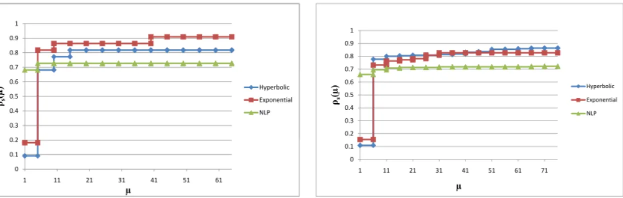
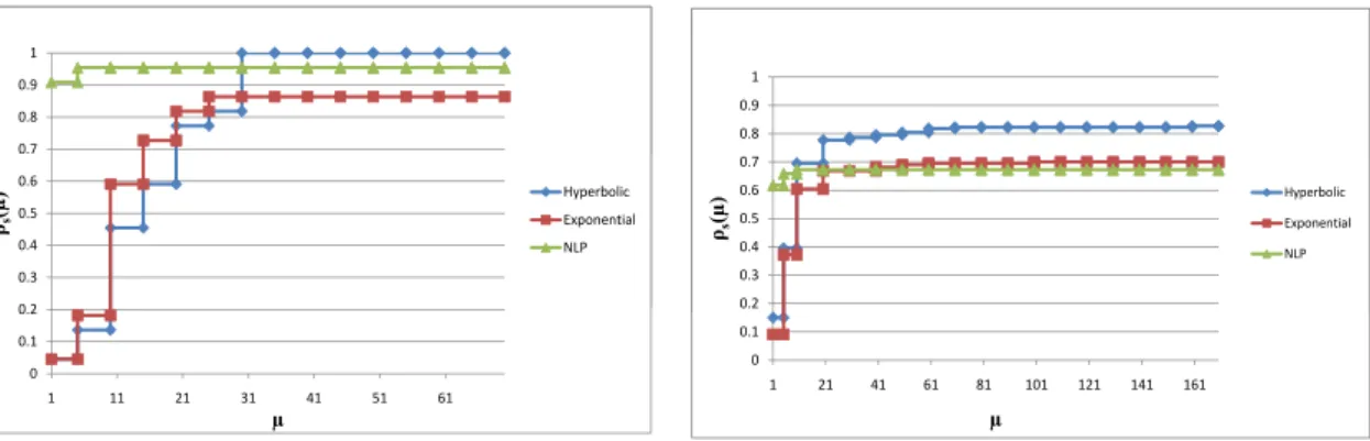
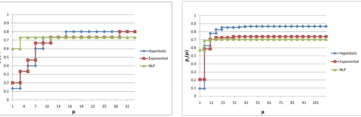
In this chapter we study hyperbolic smoothing technique in more detail. In order to apply the hy-perbolic smoothing to the finite maximum functions we represent them as a sum of maximum of two functions by adding a new variable. We study the relationship between the set of stationary points of the latter function and that of the original maximum function. The new function is approximated using hyperbolic smoothing functions and differential properties of the approximating function are studied. It is demonstrated that smooth optimization solvers can be applied to minimize the approximating function. We present results of numerical experiments using two solvers from GAMS: CONOPT and SNOPT. We also compare these results with those obtained using exponential smoothing and also nonlinear programming reformulations of minimax problems.

The structure of this chapter is as follows. We reformulate the finite maximum function in Section 3.1. Section 3.2 describes the hyperbolic smoothing function for the general maximum functions. The minimization algorithm is described in Section 3.3. Results of numerical experiments are presented in Section 3.4. Section 3.5 concludes the chapter.

3.1 Reformulation of minimax problem

In this section we will reformulate the minimax problem (2.10) to make the application of the hyperbolic smoothing to its objective function possible.

(47)

Consider the following maximum function:

f(x) = max

i∈I fi(x), I ={1, . . . , m}. (3.1)

At a pointx∈IRnconsider the set:

R(x) ={i∈I : fi(x) =f(x)}.

Using an additional variablet∈IRwe introduce the following function:

F(x, t) =t+X

i∈I

max{0, fi(x)−t}. (3.2)

For a given(x, t)the index setI can be represented as follows:

I =I1∪I2∪I3,

where

I1≡I1(x, t) ={i∈I :fi(x)< t},

I2≡I2(x, t) ={i∈I :fi(x) =t},

I3≡I3(x, t) ={i∈I :fi(x)> t}.

Denote byΨi(x, t) = max{0, fi(x)−t}, i∈I. Then for the subdifferential of the functionΨi

we have ∂Ψi(x, t) =                {0n+1}, i∈I1, co{0n+1,(∇fi(x),−1)}, i∈I2, {(∇fi(x),−1)}, i∈I3.

(48)

expression for the subdifferential ofFat the point(x, t)as follows: ∂F(x, t) ={(0n,1)}+ X i∈I1 0n+1+ X i∈I2 co{0n+1,(∇fi(x),−1)}+    X i∈I3 (∇fi(x),−1)    . (3.3)

Proposition 2. Suppose that functionsf andF are defined by (2.11) and (3.2), respectively. Then

f(x) = min

t∈IRF(x, t).

Proof. For any fixedx∈IRndefine the following function:

ϕx(t) =t+

X

i∈I

max{0, fi(x)−t}.

Observe that the functionϕxis convex piecewise linear and

ϕx(f(x)) =f(x) =F(x, f(x)).

Then the functionϕxis subdifferentiable at anyt∈IRand

∂ϕx(t) = [1− |I2| − |I3|,1− |I3|]. (3.4)

Here| · |stands for the cardinality of a set. Fort=f(x)we have thatI2 =R(x)6=∅and therefore

|I2| ≥1. Moreover for thistone hasI3 =∅and|I3|= 0. Then it follows from (3.4) that

0∈∂ϕx(f(x))

andt=f(x)is a global minimizer ofϕx. Furthermore, for any fixedx∈IRn

(49)

This completes the proof.

Proposition 3. 1) Assume that a pointx∗ ∈IRnis a stationary point off. Then(x∗, t∗)is a stationary

point of the functionF wheret∗ =f(x∗).

2) Assume that a point (x∗, t∗) is a stationary point of the function F. Then x∗ ∈ IRn is a

stationary point off.

Proof. 1) First we assume thatx∗is a stationary point of the functionf and will prove that(x∗, t∗)is a stationary point of the functionF wheret∗=f(x∗). Since

t∗ =f(x∗) = max

i∈I fi(x

∗

),

t∗ ≥ fi(x∗)for all i ∈ I and thus I3 = ∅. Moreover, I2 6= ∅ since at least one of the functions

fi, i∈Iis active atx∗. Then the subdifferential of the functionFat the point(x∗, t∗)is as follows:

∂F(x∗, t∗) ={(0n,1)}+

X

i∈I2

co{0n+1,(∇fi(x∗),−1)}. (3.5)

It is easy to see that (∇fi(x∗),0) ∈ ∂F(x∗, t∗). It is also obvious that R(x∗) = I2 at the point

(x∗, t∗). Sincex∗ is a stationary point of the functionf we get that 0n ∈ co{∇fi(x∗) : i ∈ I2}.

Then there existsλi, i∈I2such that

0n= X i∈I2 λi∇fi(x∗), λi ≥0, X i∈I2 λi = 1. (3.6)

The subdifferential∂F(x∗, t∗)is a polytope and it follows from (3.5) that points(∇fi(x∗),0), i∈I2

are among extreme points of this polytope. Then (3.6) implies that0n+1 ∈ ∂F(x∗, t∗), that is the

point(x∗, t∗)is stationary for the functionF.

2) Now assume that (x∗, t∗)is a stationary point of the functionF. We will prove that x∗ is a stationary point of the functionf. There are three cases: