New Solution Approaches for the Quadratic Assignment
Problem
Franklin Djeumou Fomeni
University of the Witwatersrand, Johannesburg School of Computational and Applied Mathematics
Supervised by: Professor Montaz Ali, University of the Witwatersrand, South Africa September 12, 2011
Declaration
I, the undersigned, hereby declare that the work contained in this dissertation is my original work, and that any work done by others or by myself previously has been acknowledged and referenced accordingly. It is being submitted for the degree of Masters of Science at the University of the Witwatersrand, Johannesburg. It has not been submitted before for any degree or examination to any other university.
———————————— Franklin Djeumou Fomeni September 12, 2011
Acknowledgements
I acknowledge the almighty God for the strength He gives me and for His love.
I am very thankful towards my supervisor Professor Montaz Ali who drew my attention to this area of optimization, for his encouragement and his guidance throughout this work. I thank both him and his visitor Dr Elzain of the university of Khartoum for suggesting the way of generating initial strictly feasible solution for the interior point method reported in this dissertation.
My sincere gratitude goes to the African Institute for Mathematical Sciences (AIMS) and the School of Computational and Applied Mathematics (CAM) for their financial support without which this dissertation would not have been possible.
I am indebted to all the staff members of the School of Computational and Applied Math-ematics of the University of the Witwatersrand, for their friendship and assistance, and particularly Prof Momoniat, Prof Banda, Dr Moitsheki, Mrs B. Pickering and Mrs D. Bowes for their supports and advices.
I gratefully acknowledge CAM’s higher degree students for their warm friendship and collab-oration, especially, Naval, Charles, Morgan, Guo-Dong, Innocent, Tumelo, Obakeng, Asha, Dario, Sima, Elimboto, Viren, Terry, Tanya, Gideon, Byron and Rahab.
I am extremely grateful to my former lecturers at the University of Yaounde I in Cameroon, especially Prof F. Wamon, Dr B. Tchapnda , Dr G. M. Mbakop, Dr Y. Emvudu for the strong mathematical background they gave me, and for their continual advices.
To my family relatives, my dear mum Clementine Tientcheu, my dad Barthelemy Tayou, the family Bakam, the family Tayo, Hugue, Chritel, Edith, and my friends, Ludovic, Lydienne, Jeanne, Alain Julio, Silver, Diane, Chrystelle, Bertin, Bruno, Thierry, Daniel, Billy, Frank, Fleur, Ronald, Danielle, Alain, Francine, Arnaud, Tafadzwa and Stephane, I say thanks for their unconditional encouragement and love. Thanks to St Francis-Xavier Martindale, Holy Trinity, Braamfontein Catholic churches for the spiritual support.
Finally, I thank the Family Ketcha for encouraging and advising me.
Abstract
A vast array of important practical problems, in many different fields, can be modelled and solved as quadratic assignment problems (QAP). This includes problems such as university campus layout, forest management, assignment of runners in a relay team, parallel and distributed computing, etc. The QAP is a difficult combinatorial optimization problem and solving QAP instances of size greater than 22 within a reasonable amount of time is still challenging. In this dissertation, we propose two new solution approaches to the QAP, namely, a Branch-and-Bound method and a discrete dynamic convexized method. These two methods use the standard quadratic integer programming formulation of the QAP. We also present a lower bounding technique for the QAP based on an equivalent separable convex quadratic formulation of the QAP. We finally develop two different new techniques for finding initial strictly feasible points for the interior point method used in the Branch-and-Bound method. Numerical results are presented showing the robustness of both methods.
Symbols nomenclature
• QAP: Quadratic assignment problem.
• RSQIP: Reformulated standard quadratic integer programming formulation of the QAP.
• SQIP: Standard quadratic integer programming formulation of the QAP.
• SCQIP: Separable convex quadratic integer programming formulation of the QAP. • CQIP: Convex quadratic integer programming formulation of the QAP.
• M ILP: Mixed integer linear programming formulation of the QAP. • QIP: Quadratic integer programming formulation of the QAP. • T F: Trace formulation of the QAP.
• KF: Kronecker formulation of the QAP. • CR1: Continuous relaxation of (RSQIP). • CR2: Continuous relaxation of (SCQIP). • BL: Barrier logarithmic problem.
• AN LIP: Auxiliary non-linear integer programming problem from (RSQIP). • GA: Genetic algorithm.
• ACO: Ant colony optimization. • SA: Simulated annealing. • TS: Tabu search.
• DDC: Discrete dynamic convexized.
Contents
Declaration i Acknowledgements ii Abstract iii Symbols nomenclature iv 1 Introduction 11.1 Mathematical formulation of the optimization problem . . . 2
1.2 The Quadratic Assignment Problem . . . 4
1.3 Methods for solving the QAP . . . 5
1.4 Structure of the dissertation . . . 6
2 Mathematical background 7 2.1 The quadratic form . . . 7
2.2 Matrix analysis . . . 9
3 Literature review 17 3.1 Formulations of the QAP . . . 17
3.1.1 Quadratic integer programming formulation . . . 17
3.1.2 Trace formulation . . . 18
3.1.3 Kronecker formulation . . . 19
3.1.4 Mixed integer linear programming (MILP) formulation. . . 19
3.2 Applications of the QAP . . . 20
3.3 The lower bounding techniques . . . 22
3.4 Solution methods for the QAP . . . 25
4 Problem formulation and lower bounding techniques 29 4.1 Standard quadratic integer programming formulation (SQIP) . . . 29
4.2 Separable quadratic integer programming formulation . . . 32
4.3 Lower bounds via the continuous relaxation of (RSQIP). . . 33
4.4 Lower bounds via the continuous relaxation of (SCQIP). . . 34
4.4.1 An interior point algorithm for (CR2) . . . 35
4.4.2 Discussions of the interior point algorithm . . . 38
5 Finding a starting point for the interior point algorithm 43 5.1 Description of the first technique . . . 43
5.1.1 The first step . . . 43
5.1.2 The second step . . . 45
5.2 Description of the second technique. . . 46
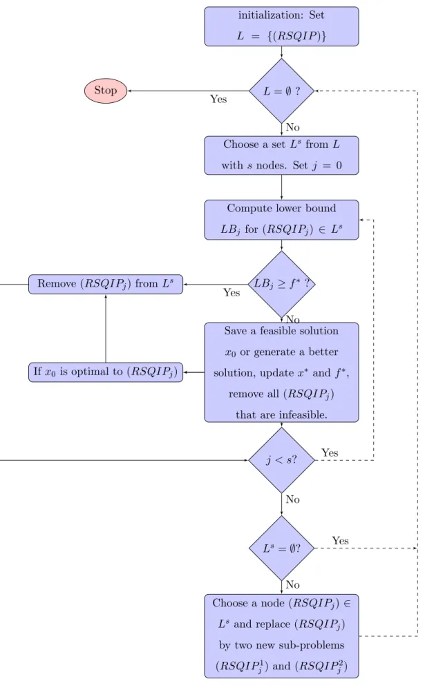
6 New methods for solving the QAP 48 6.1 The Branch-and-Bound method for the QAP . . . 48
6.1.1 Choice of the branching variables . . . 50
6.1.3 TheBranch-and-Bound algorithm . . . 53
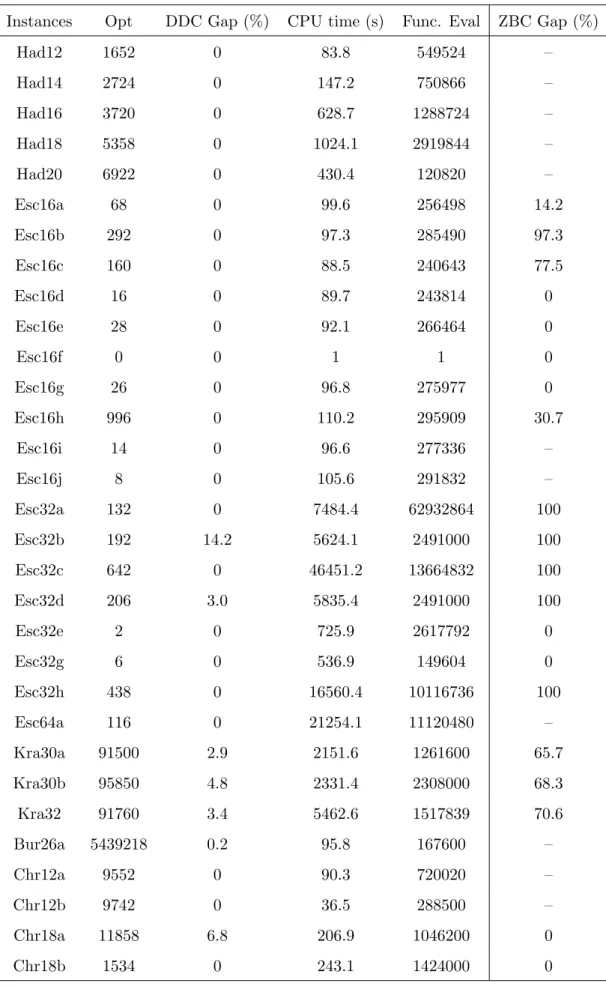
6.2 An auxiliary function-based dynamic convexized method . . . 55
6.2.1 The auxiliary function and its properties. . . 56
6.2.2 The discrete dynamic convexized (DDC) algorithm . . . 62
7 Numerical experiments and results 65 7.1 Computation of lower bounds . . . 65
7.2 A heuristic random enumeration . . . 68
7.3 Implementation of theBranch-and-Bound algorithm . . . 69
7.4 Implementation of the auxiliary function-based method . . . 71
8 Conclusion and further research 82 9 Appendix 84 9.1 Appendix 1: Generalized inverse of a matrix. . . 84
9.2 Appendix 2: Minimizers from the auxiliary function-based method . . . 85
9.3 Appendix 3: Choice of the value of N in the random enumeration . . . 89
List of Figures
1.1 Local optima vs global optima . . . 3
6.1 The Branch-and-Bound flow chart . . . 54
7.1 . . . 78 7.2 . . . 79 7.3 . . . 80 7.4 . . . 81 9.1 . . . 90 9.2 . . . 91 9.3 . . . 92 9.4 . . . 93 viii
List of Tables
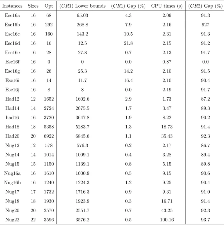
7.1 Lower Bounds from the continuous relaxation of (RSQIP) . . . 67
7.2 Results from the Branch-and-Bound algorithm: Part 1 . . . 74
7.3 Results from the Branch-and-Bound algorithm: Part 2 . . . 75
7.4 Results from the auxiliary function-based method: Part 1 . . . 76
7.5 Results from the auxiliary function-based method: Part 2 . . . 77
9.1 Minimizers of the solutions from the auxiliary function-based method (1) . 86
9.2 Minimizers of the solutions from the auxiliary function-based method (2) . 87
9.3 Minimizers of the solutions from the auxiliary function-based method (3) . 88
1. Introduction
Optimization is an important tool in decision science and in analysis of physical systems. It has application in all branches of Science, Engineering and Management. In nature, physical systems tend to state of minimum energy. The molecules in an isolated chemical system react with each other until the total potential energy of their electron is minimized. Rays of light follow paths that minimize their travel time. Manufacturers aim for maximum efficiency in the design and operation of their production processes. Airline companies schedule crews and aircraft to minimize cost. Investors seek to create portfolios that avoid excessive risks while achieving a high rate of return.
To use optimization, one first needs to identify some objective, which is a quantitative measure of the performance of the system under consideration. This objective could be, the cost, the profit, the time, the potential energy or any quantity or combination of quantities that can be represented by a number. The objective depends on certain characteristics of the system, called variables. In an optimization problem, one’s goal is to find the values of the variables that optimize the objective. In most of the cases, There are constraints in the problem that restrict the values of the variables. The feasible set of the problem is determined by the constraints. Optimization is divided into continuous, discrete and mixed integer programming. In the continuous optimization, the variables used in the objective can assume real values. Continuous optimization comprises linear programming and non-linear programming. A continuous optimization is convex if the objective is a convex1 function of the variables and the feasible set is also convex.
As opposed to continuous optimization, the variables used in the discrete optimization are restricted to assume only discrete values, such as the integers. There are two notable branches of discrete optimization, namely, combinatorial optimization, in which the feasi-ble set is a finite subset of the set of all the integer numbers, and integer programming in
1
Details and characteristics of a convex function are given in Chapter2
Section 1.1. Mathematical formulation of the optimization problem Page 2
which variable are simply constrained to assume only integer values. Discrete optimization problems can also be formulated as a linear, non-linear, convex or non-convex optimization problem. Mixed integer optimization combines both real and integer variables. This disser-tation deals with a combinatorial optimization problem, namely, the quadratic assignment problem.
1.1
Mathematical formulation of the optimization problem
Mathematically speaking, optimization is concerned with finding the maxima or minima of a function subject to restrictions on its variables. An optimization problem is a problem of the formmin
x∈S f(x), (1.1)
wherexstands for the variables,Sis the feasible set or the feasible set, andf :S ⊆Rn−→Y with Y ⊆Ris the objective function. The feasible set is defined by S ={x ∈Rn:g(x)≥
0, h(x) = 0}, whereg(x), h(x) are also real-valued funtions.
If the search space S is continuous, then we have a continuous optimization problem, if it is discrete, then we have a discrete optimization problem.
Definition 1.1.1 (Feasible and strictly feasible points): A pointx∈Rn is said to be feasible for (1.1) ifx∈S.
If the interior of S is non empty, x is said to be strictly feasible for (1.1) if x is in the interior ofS.
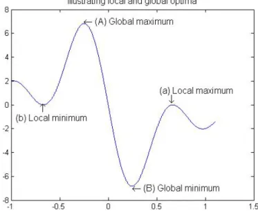
Definition 1.1.2 (Local minimum, local maximum):
A point x∗ ∈ S is said to be a local minimum (local maximum) of f if f(x∗) ≤ f(x)
(f(x∗) ≥ f(x)) for all x in a neighbourhood of x∗. In other words, this means that there exists ε >0 such that f(x∗)≤f(x) (f(x∗)≥f(x)) and kx∗−xk< ε, x∈S.
Section 1.1. Mathematical formulation of the optimization problem Page 3
Definition 1.1.3 (Global minimum, global maximum):
A pointx∗ is said to be a global minimum (global maximum) iff(x∗)≤f(x) (f(x∗)≥f(x))
for all x∈S.
Definition 1.1.4 (Optima):
A pointx∗∈S is called an optimizer of f if x∗ is a minimizer or a maximizer of f.
Figure1.1gives a graphical illustration of local and global optima. In this figure, the points (A) and (B) are global maximum and minimum respectively. While the points (a) and (b) are local maximum and minimum respectively. The global maximum (Minimum) is also a local maximum (Minimum).
Section 1.2. The Quadratic Assignment Problem Page 4
1.2
The Quadratic Assignment Problem
The QAP is one of the fundamental combinatorial optimization problems. It was introduced in 1957 by Koopmans and Beckmann [KB57] as a mathematical model for the location of a set of indivisible economical activities. The QAP considers the problem of allocating a set ofnfacilities to a set ofnlocations, with the cost being a function of the distance and flow between facilities, plus costs associated with a facility being placed at a certain location. The formal definition of the problem is as follows. Let n be the number of facilities and locations,F = (fij)1≤i,j≤n, D= (dkl)1≤k,l≤n and B = (bik)1≤i,k≤n be three n×nmatrices, where fij is the flow between the facilities i and j, dkl, the distance between the locations
k and l, andbik the cost of the facility i being placed at the location k. Let Sn be the set of all the permutations φ:{1, . . . , n} −→ {1, . . . , n}, see Definition 2.2.15 in Chapter2. The QAP was originally defined as follows:
min φ∈Sn n X i=1 n X j=1 fijdφ(i)φ(j)+ n X i=1 biφ(i). (1.2)
The termbiφ(i)in (1.2) is the cost associated with placing facilityiat locationφ(i). On the other hand, the productfijdφ(i)φ(j) represents the cost of placing facilityj at locationφ(j) while facility iis placed at location φ(i).
A lot of interests have been given to the QAP since its introduction in 1957. The QAP has been used as the mathematical model of many real life problems arising in facility location, computer manufacturing, scheduling, building layout design, process communications, etc. Indeed, in Chapter 3 we review some of the direct applications of the QAP in real life. Solving the QAP using exact solution methods is still a challenge. In fact, many problem instances of size n > 20 are still found difficult to be solved with exact algorithm within reasonable computational time. Sahni and Gonzalez [SG76] have shown that the QAP is NP-hard and that even finding an approximate solution within some constant factor from the optimal solution cannot be done in polynomial time unless P=NP.
Section 1.3. Methods for solving the QAP Page 5
1.3
Methods for solving the QAP
The different methods used to achieve a global optimum for the QAP include Branch-and-Bound, cutting planes, Branch-and-Cut, and semi-definite programming (SDP). However, the aim of this dissertation is to develop new solution approaches for the QAP. We identify a mathematical formulation of the QAP, which has not been studied in the literature yet, for which we develop two solution methods. Our first solution method is aBranch-and-Bound
method which is a systematic enumerative scheme that uses lower bounds to eliminate undesired solutions.
Our second solution method is an auxiliary function-based dynamic convexized method. This method consists of building a sequence of minimizers, using a local search algorithm, for the QAP which converges towards the optimum solution of the problem. The dynamic convexized method incorporates some mechanisms that allow it to escape from local minima. It has recently been proposed by Zhu and Ali [ZA09] for solving the general non-linearly constrained non-linear integer programming, and has never been applied to the QAP. This dissertation offers the first application of this method to the QAP. Central to the application of dynamic convexzied method to the QAP is a neighbourhood structure of the QAP that we introduce. This makes the dynamic convexzied method different from the one proposed by Zhu and Ali [ZA09].
In order to improve the efficiency and speed up the convergence of the two solution meth-ods, we have proposed a heuristic random enumerative scheme to identify an initial solution with which to start the new methods proposed in this dissertation. Another major contri-bution in this dissertation is the identification of a strictly feasible solution of the quadratic formulation of the QAP. We have developed two different techniques for finding an initial strictly feasible point for the interior point method, since we used an interior point algo-rithm for our lower bounding technique in the Branch-and-Bound. These two techniques can consequently be applied to other interior point algorithms.
Section 1.4. Structure of the dissertation Page 6
1.4
Structure of the dissertation
The rest of this dissertation is organized as follows:• In Chapter2, we present the mathematical background necessary for the understand-ing of this dissertation.
• In Chapter 3, we review the previous developments in the area of the QAP. This review comprises the different mathematical formulations of the QAP, its applications to real life problems, the existing lower bounding techniques and the existing solution methods.
• Chapter 4, we present a standard quadratic integer programming (RSQIP) formu-lation of the QAP. This is a reformuformu-lation of the standard quadratic integer pro-gramming (SQIP) formulation suggested in [BcPP98]. We then transform this stan-dard quadratic integer programming reformulation, (RSQIP), into a separable convex quadratic integer programming (SCQIP) problem using a decomposition technique. We study (RSQIP) and (SCQIP) in this dissertation. Two lower bounding tech-niques based on these two problem formulations are also presented in this chapter.
• In Chapter5, we develop two different techniques for finding an initial strictly feasible point for the interior point method.
• In Chapter 6, we present in detail the two new solution approaches proposed in this dissertation together with the step-by-step descriptions of the corresponding algo-rithms.
• In Chapter 7, the details of the numerical experiments and a full set of numerical results from the two solution methods are presented.
2. Mathematical background
Since the introduction of the QAP, researchers have been using mathematical theories to advance the reformulations and approximations of the QAP. Reformulations and ap-proximations are used to design algorithms for the QAP. In this dissertation, we develop some mathematical theories and suggest new algorithms for solving the QAP. This chapter presents some mathematical tools useful for an easy understanding of various reformula-tions and approximation of the QAP. We begin with some basic notareformula-tions used throughout the dissertation: Rn ,Zn and Qn denote the set of all real, integer and rational n-vectors,
respectively;Rm×n ,Zm×nandQm×n denote the set of all real , integer and rationalm×n
matrices, respectively. The set of all positive integers is also denoted by Z+ and the set of all rational numbers by Q. The upper script T to any vector or matrix stands for its
transpose.
2.1
The quadratic form
Definition 2.1.1 (Bilinear function): A function
f :E×F −→G, i.e.
(x, y)7−→f(x, y), E ⊆Rm, F ⊆
Rn and G ⊆Rq, m, n, q ∈Z+, is called a bilinear function if it is linear in
each of its variables i.e for all x, x1, x2∈E, y, y1, y2 ∈F and a, b∈Rwe have:
• f(ax1+bx2, y) =af(x1, y) +bf(x2, y), • f(x, ay1+by2) =af(x, y1) +bf(x, y2).
In addition, if E=F, thenf is said to be symmetric iff(x, y) =f(y, x) for allx, y∈E. 7
Section 2.1. The quadratic form Page 8
Definition 2.1.2 (Bilinear form):
A bilinear function f is said to be a bilinear form if Gis reduced to R i.e.
f :E×F −→R.
Definition 2.1.3 (Quadratic form): A quadratic form over E is a function
q:E−→R, i.e. x7−→q(x)
such thatq(x) =f(x, x), where f(•,•) is a symmetric bilinear form overE; f is called the associated bilinear form of q.
Given a quadratic form q, its associated bilinear form f can always be retrieved from q as follows:
f(x, y) = 1
2(q(x+y)−q(x)−q(y)). Any quadratic form q is fully defined by its matrix M i.e.
q(x) = 1 2x
TM x.
Definition 2.1.4 (Positive semi-definiteness and positive definiteness): A matrix M is said to be positive semi-definite if:
xTM x≥0,∀x∈Rm,
it is said to be positive definite if
xTM x >0,∀x∈Rm\ {0}.
Definition 2.1.5 (Convex function):
Let g be a real valued function defined overE ⊆Rn. The function g is said to be a convex
function if it satisfies:
Section 2.2. Matrix analysis Page 9
for all x, y∈E andt∈[0,1], it is said to be strictly convex if
g(tx+ (1−t)y)< tg(x) + (1−t)g(y)
for all t∈(0,1).
It is well known [Cot67] that a quadratic form q(x) =xTM x is convex if its matrix M is positive semi-definite, it is strictly convex ifM is positive definite.
2.2
Matrix analysis
Definition 2.2.1 (Rational elementary row and column operations):
For a rational matrix, the rational elementary row or column operations are:
i) Interchanging two rows or two columns.
ii) Multiplying a row or a column by a non-zero rational number.
iii) Adding a rational multiple of one row (or one column) to another row (or column). Theorem 2.2.2:
Let M be an n×n rational symmetric matrix such that a zeros pivot is never encoun-tered when applying Gaussian elimination with type iii) operations, then there exists a non-singular rational matrix P such that
PTM P =diag( ¯d1, . . . ,d¯n). (2.1)
Proof. LetM be ann×nrational symmetric matrix such that the hypothesis of Theorem
2.2.2 holds . It is well known (Chapter 3 of [Mey00]) that by performing a sequence of rational elementary row and column operations on M, one can decomposeM as M =LU
Section 2.2. Matrix analysis Page 10
matrix and U is an upper triangular matrix, both with non-zero elements on the main diagonal.
It follows from theLU factorization thatUT =L
1U1, where U1 is a diagonal matrix, since all the elements in the upper triangular half of UT are equal to zero, while L1 is a lower triangular matrix.
Therefore we can write M = LU1LT1. Given that M is a symmetric matrix, we have
MT = M ⇐⇒ L1U1LT = LU1LT1 i.e L = L1, since the same elementary operations that are applied to each row will also be applied to the corresponding column.
Hence, if we chooseP = L−1T
and ¯D=U1,Theorem2.2.2holds, where ¯D=diag( ¯d1, . . . ,d¯n).
When transforming the objective function of a quadratic integer programming problem into a separable1 quadratic form, it is desirable that the resulting quadratic program keeps the integral nature.
Considering a quadratic form q(x) = 1 2x
TM x+cTx where M is such that PTM P =
diag( ¯d1, . . . ,d¯n), as in Theorem2.2.2. We set x=P y⇐⇒y =P−1x, then the quadratic formq becomesq(y) = 1 2(P y) TM(P y) +cT(P y) = 1 2y T(PTM P)y+cTP y= 1 2y TDy¯ + ¯cTy with ¯cT = cTP. The new variable y will be ensured to be integral if P−1 is an integer matrix.
Definition 2.2.3 (Congruent matrices):
A matrix A is said to be congruent to a matrix B if there exists a non-singular matrix P
such that PTAP =B. The matrix P is called the congruent matrix of A and B.
The congruence relation is an equivalence relation. Indeed we have:
• ITAI =A i.e the congruence relation is reflexive.
• PTAP =B ⇐⇒(P−1)TB(P−1) =A, the relation is symmetric.
1
Section 2.2. Matrix analysis Page 11
• PTAP = B and QTBQ = C =⇒ (P Q)TA(P Q) = C, with (P Q)−1 = Q−1P−1, the relation is transitive.
Definition 2.2.4 (Unimodular matrix):
A matrix U ∈Rn×n is unimodular if it is integral and det(U) =±1, where det(U) denotes
the determinant of U.
It is easy to see that a matrixP isunimodular if and only ifP−1 isunimodular. Therefore ifP is unimodular, then P y∈Zn⇐⇒y∈Zn. Hence for a quadratic integer programming
problem that hasq(x) = 1 2x
TM x+cTxas the objective function, the transformed separable quadratic program with the objective function q(y) = 1
2y
TDy¯ + ¯cTy, x = P y, D¯ =
PTM P, will be an integer optimization problem as well. However, such a unimodular
congruence transformation does not always exist for all the rational symmetric matrices.
Example 2.2.5: Let M = 0 1 1 0 ,
and suppose that there is an integer matrix
P = a b c d
such that PTM P is diagonal. Then, we must have bc+ad = 0 and ad−bc =±1, which implies 2ad=±1, a contradiction that aand dare both integer numbers. Thus, there does not exist a unimodular congruence transformation for M.
Definition 2.2.6 (Semi-unimodular matrix):
A matrix P is said to be semi-unimodular if P−1 is an integer matrix.
Let us suppose thatP is asemi-unimodular matrix, thereforeP y∈Zn⇐⇒y∈
Section 2.2. Matrix analysis Page 12
For a rational symmetric matrixM with non-zero pivots using typeiii) rational elementary operations under Gaussian elimination, Zheng et al [ZSL10] proposed a procedure of ob-taining asemi-unimodular congruent matrixP such that PTM P is diagonal. Their result is stated in the following theorem.
Theorem 2.2.7 (Integer diagonalisation):
For any rational symmetric matrix M such that the hypothesis of Theorem 2.2.2 holds, there exists a semi-unimodular congruent matrix P such that
PTM P =diag(d1, . . . , dn) (2.2)
Proof. NB: The proof of this theorem is the same as that in [ZSL10].
Let Di(k) be the elementary matrix obtained by multiplying the i–th row of the identity matrix by k and Tij(k) be the matrix obtained by adding k times of the j–th row to the
i–th row of the identity matrix, where kis a rational number.
It follows from2.2.2that there exists a non-singular rational matrixV such thatVTM V =
diag( ¯d1, . . . ,d¯n). Since the elements of M are rational, the elements k in the elementary matrices Di(k) and Tij(k) involved in V are also rational. Thus each element of V−1 is rational. If V−1 is an integer matrix, thenP =V satisfies (2.2). Suppose now thatV−1 is not an integer matrix. Let all the entries of V−1 be written as (vulgar) fractions. Let ki be the least common denominator (lcd) of the i–th row of V−1. Here, we set ki = 1 if all entries of thei–th row are integers. Let
P =V D1 1 k1 . . . Dn 1 kn , then P−1 =Dn(kn). . . D1(k1)V−1 is an integer matrix and
PTM P =diag(d1, . . . , dn), wheredi= ¯di/ki2, i= 1, . . . , n.
Section 2.2. Matrix analysis Page 13
Definition 2.2.8 (Diagonally dominant matrix):
A matrix M = (mij)1≤i,j≤n is said to be diagonally dominant if for every row and column
of M the magnitude of the diagonal entry in a row and column is greater than or equal to the sum of the magnitudes of all other (non-diagonal) entries in the same row and column. In other words, M is diagonally dominant if |mii |≥ P
j6=i
|mij | for all i= 1, . . . , n, M is
strictly diagonally dominant if |mii|> P j6=i
|mij |for all i= 1, . . . , n.
Lemma 2.2.9:
If a matrix M is diagonally dominant with real non-negative diagonal entries, then it is positive semi-definite.
Proof. This lemma is a direct consequence of the Gerschgorin’s circle theorem [S.G31].
Lemma 2.2.10:
In addition to the assumptions ofTheorem 2.2.7, if the matrix M is diagonally dominant then there exists a semiunimodular congruence matrixP such thatPTM P =diag(d1, . . . , dn)
and di ≥0 for all i= 1, . . . , n.
Proof. In the proof of Theorem 2.2.7, the matrixdiag(d1, . . . , dn) is obtained from (2.1) by the relation di = ¯di/ki2 for some rational number ki, i = 1, . . . , n. So to end our proof, it is sufficient to show that if M is diagonally dominant, then every element ¯di in (2.1) is positive. To do so we consider the Gaussian elimination that leads to (2.1), and show that every diagonal element remains positive. Given that the matrix M is non-zero and diagonally dominant, there is no need of interchanging two rows or columns. There is also no need to multiply a row or a column by a non-zero rational number. Thus the only rational elementary operations involved in the Gaussian elimination are operations of type
iii), which corresponds to, for a row Rj, Rj ←−Rj+αRi withα∈Q∗ =Q\ {0}.
If the pivot is fixed at the diagonal entry Mii (which is already positive) on the row Ri, then for any other row Rj, j > i, we will have Rj ←−Rj−
Mji
Mii
Section 2.2. Matrix analysis Page 14
on the rowRj will becomeMjj−
Mji
Mii
Mij. We consider the two cases below:
• IfMij ≤0, thenMjj− Mji Mii Mij ≥0 since|Mji |≤Mii and |Mij |≤Mjj. • IfMij >0, sinceMji≤Mii, therefore Mjj− Mji Mii Mij ≥Mjj−Mij ≥0.
Thus every diagonal entry of the resulting matrix will be left positive. Hence ¯di ≥ 0 for
i= 1, . . . , n.
Theorem 2.2.11 (Eigenvalue factorization):
Let M be an n×n symmetric matrix, there exists an orthogonal matrix P such that
M =PTDP, where D is a diagonal matrix with eigenvalues of M on the diagonal. Definition 2.2.12 (Trace of a matrix):
The trace of ann×nmatrixM denoted bytr(M) is the sum of all the element on its main diagonal, i.e. tr(M) = n X i=1 mii.
Given any twon×n-matricesF andD, some well known properties of the trace are given by:
• tr(F D) =tr(DF), • tr(F) =tr(FT),
• forF =FT and for anyn×n-matrix X, we havetr(F XDTXT) =tr(F XDXT).
Definition 2.2.13 (Kronecker product):
Section 2.2. Matrix analysis Page 15
B, denoted A⊗B, is defined by:
A⊗B = a11B a12B . . . a1nB . . . . . . . . . am1B am2B . . . amnB
which is the mp×nq matrix formed from all possible pairwise element products of A and
B. Example 2.2.14: A= 1 2 2 4 3 1 and B = 5 1 1 2 then A⊗B = B 2×B 2×B 4×B 3×B B (2.3) = 5 1 10 2 10 2 1 2 2 4 2 4 20 4 15 3 5 2 4 8 3 6 1 2 . (2.4) Definition 2.2.15 (Permutation):
A permutation of the set {1, . . . , n} is a one-to-one correspondence from {1, . . . , n} onto itself.
Definition 2.2.16 (Permutation matrix):
A permutation matrix is a square binary matrix that has exactly one entry 1 on each row and each column and 0’s everywhere else. We denote by Xn the set of all permutation matrices of size n×n.
Section 2.2. Matrix analysis Page 16
Definition 2.2.17 (Vector norm):
Let E be a sub-vector space of Rn. A norm on E is an application ρ : E −→ R which
satisfies the following properties:
i) ρ(x)≥0, for all x∈E,
ii) ρ(ax) =|a|ρ(x), for all x∈E and a∈R,
iii) ρ(x+y)≤ρ(x) +ρ(y), for all x, y∈E, iv) If ρ(x) = 0, then x= 0.
On the vector spaceRn, we define the the following norms:
• kxk1= n P i=1
|xi |, it is called the Taxicab norm.
• kxk2= n P i=1 x2i 1/2
, it is called the Euclidean norm.
• kxk∞= max
3. Literature review
In this chapter, we present a review on the QAP so that the reader can see how different is the current work to what have been done in this area already. Since its introduction, the QAP has gained a lot of attentions from researchers all over the world. This is due to its applications in a wide range of applied areas and its challenging difficulty. In this chapter, we review some important mathematical reformulation of the QAP, some of the real life applications of the QAP, the lower bounding techniques used in different solution approaches, and finally the exact and heuristic solution methods that have been adopted for the QAP.
3.1
Formulations of the QAP
Since its introduction, the QAP has been formulated in many different ways ranging from the linear form to the SDP form. Here we present some selected mathematical formulations.
3.1.1 Quadratic integer programming formulation
Considering the fact that for every permutation of{1, . . . , n}, there is a corresponding ele-mentXinXn, whereX= (xij)1≤i,j≤n. The permutationφin the original QAP formulation (1.2) can therefore be replaced by a permutation matrix X= (xij)1≤i,j≤n where
xij =
1 if facilityiis placed at location j,
0 otherwise.
(3.1)
Using this notation, Koopmans and Beckmann [KB57] gave the following quadratic integer programming formulation: (QIP) min n X i=1 n X j=1 n X k=1 n X l=1 fijdklxikxjl+ n X i=1 n X j=1 bijxij, s.t. (3.2) 17
Section 3.1. Formulations of the QAP Page 18 n X i=1 xij = 1 forj= 1, . . . , n, (3.3) n X j=1 xij = 1 fori= 1, . . . , n, (3.4) xij ∈ {0,1} fori, j= 1, . . . , n, (3.5) where fij is the flow between facility iand facility j, dkl the distance between location k and location l and bij the cost of placing facility i at location j. This formulation can be found in most of the linearisation approaches for the QAP.
3.1.2 Trace formulation
Considering a QAP instance with flow matrixF, distance matrixDand cost matrixB, we set ¯D=XDTXT, which leads to ¯dji =dφ(i)φ(j) fori, j= 1, . . . , n. It then follows that
tr(F XDTXT) =tr(FD¯) = n X i=1 n X j=1 fijd¯ji = n X i=1 n X j=1 fijdφ(i)φ(j),
whereφ is the permutation associated with the permutation matrixX.
Therefore the original formulation of the QAP can equivalently be reformulated in the following form:
min tr(F XDT +B)X, s.t. (3.6)
X ∈ Xn, (3.7)
which is equivalent to
Section 3.1. Formulations of the QAP Page 19
XTe=e, (3.9)
Xe=e, (3.10)
xij ∈ {0,1} for all i, j, (3.11) where e is the column n–vector of ones. This formulation was introduced by Edward [Edw80]. The spectral theory was applied to this formulation to develop the eigenvalue lower bounding and some other lower bounding techniques, see [FBR87,HRW90,Had94,KR95].
3.1.3 Kronecker formulation
Given ann×n-matrix X, we define vec(X) to be the n2-vector formed by the columns of
X. The QAP can thus be formulated as:
(KF) min xT(F ⊗D)x+bTx, s.t. (3.12)
XTe=e, (3.13)
Xe=e, (3.14)
xi∈ {0,1}for all i= 1, . . . , n2, (3.15) wherex=vec(X) andb=vec(B). This formulation was suggested in a survey by Burkard et al. [PRW94] in 1994 but has not been studied further.
3.1.4 Mixed integer linear programming (MILP) formulation
In the MILP formulation, the QAP formulation (3.2)–(3.5) is simplified by adding some new variables, see [LW76]. These variables together with the MILP formulation are pre-sented below. Let us consider the objective function of the quadratic integer programming formulation given by equation (3.2). In this function, we set Cijkl =fijdkl ifi6=j ork6=l
Section 3.2. Applications of the QAP Page 20
and Ciikk =fiidkk+bik. The new variables are now defined as yijkl=xikxjl fori, j, k, l= 1, . . . , n and the QAP is transformed into the following MILP:
(M ILP) min n X i=1 n X j=1 n X k=1 n X l=1 Cijklyijkl, s.t. (3.16) n X i=1 xik = 1 fork= 1, . . . , n, (3.17) n X k=1 xik = 1 fori= 1, . . . , n, (3.18) n X i=1 yijkl=xjl forj, k, l= 1, . . . , n, (3.19) n X j=1 yijkl=xik fori, k, l= 1, . . . , n, (3.20) n X k=1 yijkl=xjl fori, j, l= 1, . . . , n, (3.21) n X l=1 yijkl=xik fori, j, k = 1, . . . , n, (3.22) xij ∈ {0,1} fori, j= 1, . . . , n, (3.23) yiikk=xik fori, k = 1, . . . , n, (3.24) 0≤yijkl ≤1 fori, j, k, l= 1, . . . , n. (3.25)
3.2
Applications of the QAP
The QAP was originally introduced by Koopmans and Beckmann [KB57] to model the assignment of activities in economy. Afterwards, the QAP has been successfully used to model problems arising from many different areas. For example, the QAP has been applied in the backboard wiring. The backboard wiring is concerned with placing the computer’s elements on the backboard while minimizing a bounded numeric norm. The norm is
cal-Section 3.2. Applications of the QAP Page 21
culated as the product of the inter-connexion between the elements, and the length of wire needed to connect elements placed at given positions. The problem was casted into math-ematical formulation by Steinberg [Ste61]. As an application of mathematics in sports, Heffley [Hef77] pointed out that the assignment of runners in a relay team leads to the QAP. Geoffrion and Graves [GG76] used a quadratic assignment formulation to treat the problem of scheduling parallel production lines with changeover costs. Here the production orders for a number of products must be scheduled on a number of production lines, so as to minimize the sum of products costs. The total cost consists of the changeover costs, pro-duction costs and the cost involving time restrictions. Pollatscheck et al. [PGR76], on the other hand, used the QAP to define the best design typewriter keyboard and control panels.
The application of the QAP in Chemistry has also been reported by Forsberg et al [FDZ+94] who used the QAP in the analysis of some chemical reactions. In the area of numerical analysis, the combinatorial solution for the least-square uni-dimensional scaling of symmet-ric proximity matsymmet-rices is known to be very sensitive to the starting point. Brusco and Stahl [BS00] proved that using the solution to a QAP as a starting point substantially improves the final seriation quality and the computational efficiency of this problem.
The QAP has a number of applications in the location problem. For example, in university
campus layout problem, where there is a need for a university to enlarge its campuses while minimizing the amount of required travel for students and staff. The QAP happened to be the solution as was mathematically formulated so by Dickey and Hopkins [DH72]. Similarly, the problem of locating hospital department with the aim of minimizing the total distance travelled by patients was formulated by Elshafei [Els77] as a QAP. Jan Bos [Bos93] used the QAP formulation to solve the zoning problem which arose in forest management. This problem is concerned with the planning of territorial structures by designating area units for specific purpose.
Section 3.3. The lower bounding techniques Page 22
In addition to the above examples, several applications of the QAP also arise in electron-ics. For example, Rabak and Schiman [RS03] showed that the problem of optimizing the automatic electronic components insertion in a particular inserting machine corresponds to a QAP. Miranda et al. [MLMF05] used the QAP formulation to model the electronic board design problem. In this problem, one needs to place electronic components to some locations in a printed circuit card so as to minimize the distance among the components that have greater levels of interactivity and energy or data flow, in order to avoid excessive signal delay. On the other hand, the index assignment which has to do with error control in communications was proved by Ben-David and Malah [DM05] to be a special case of the QAP. Wess and Zeitlhofer [WZ04] represented the problem of memory layout optimization in signal processor as a QAP. Many other QAP’s applications can be found in the literature [LAN+07].
3.3
The lower bounding techniques
Ever since the QAP was originally suggested, many researchers have been working on var-ious solution techniques [LAN+07]. The ability of some QAP instances to be solved, both exactly and approximately, depends on their lower bounding techniques. The lower bound-ing techniques are used within implicit enumeration algorithms, such asBranch-and-Bound, in order to perform a limited search of the feasible region of the problem, until an optimal solution is found. Therefore many researchers have focused on developing lower bounds for the QAP instances. Based on the mixed integer linear programming (MILP) formula-tion (3.16), Gilmore [Gil62] and Lawler [Law63] independently derived similar lower bounds (known as the Gilmore-Lawler lower bounds) for the QAP by constructing a solution matrix in the process of solving a series of linear assignment problem. The Gilmore-Lawler lower bounds have been widely used for roughly three decades because of their cheap computa-tional cost.
Section 3.3. The lower bounding techniques Page 23
Using the linear programming relaxation of the MILP formulation (3.16), Resende and Ra-makrishnan [MRD95] computed lower bounds for the QAP instances via an interior point method. In their work, they used the primal simplex algorithm and the interior point algo-rithm, both available in the commercial linear programming solver CPLEX. For about 80% of the problem instances available in the QAP library [BcKR], Resende and Ramakrishnan produced lower bounds tighter than the Gilmore-Lawler lower bounds. Another bounding technique that shares the basic idea with the Gilmore-Lawler lower bounding technique has been developed by Hahn and Grant [HG98]. This lower bounding technique is based upon a dual formulation. It extends the Hungarian algorithm [Kuh55] for the linear assignment problem to the QAPs. Karisch et al. [KR95] investigated this dual-based lower bounding technique. They revealed that it is an iterative approach in which the dual of some linear programming relaxation of the original problem is solved, and reformulated at each itera-tion. The reformulation step makes use of the information provided in the preceding step.
Given that linear programming problems are easy to solve, many researchers have focused on the MILP formulation (3.16) in order to develop good quality lower bounds. For exam-ple, Frieze and Yadegar [FY83] gave a MILP reformulation of the QAP. They studied the Lagrangian relaxation of it, and developed two sub-gradient optimization-based algorithms to approximately solve the MILP. They were able to give lower bounds better than the Gilmore-Lawler lower bounds. Adams and Johnson [AJ94] proposed another MILP refor-mulation of the QAP similar to the reforrefor-mulation idea of Frieze and Yadegar [FY83]. In their work, the number of constraints of the problem is considerably reduced compared to the MILP reformulation by Frieze and Yadegar [FY83]. Adams and Johnson obtained lower bounds simply by considering the continuous relaxation of their problem reformulation. On the other hand, Karisch et al [KR95] studied a theoretical relationship between the two lower bounding techniques by Adams and Johnson [AJ94] and Hahn and Grant [HG98]. It was reported that, unlike other Gilmore-Lawler-like bounds, the Hahn and Grant bounds cannot be obtained by applying the algorithm of Adams and Johnson (to solve the Lagrangian
re-Section 3.3. The lower bounding techniques Page 24
laxation). However, both Adams and Johnson [AJ94] and Hahn and Grant [HG98] bounds can be obtained as feasible solutions of the dual of the continuous relaxation of the mixed integer linear programming reformulation by Adams and Johnson.
In 1990, Hadley et al. [HRW90] used the trace formulation (3.6) to develop the projection lower bound for the QAP. They obtained additional improvements by making an efficient use of a tractable representation of the orthogonal matrices having constant row and col-umn sum. Based on the relationship of the objective function of the trace formulation (3.6) and the eigenvalues of its coefficient matrices, Finke et al.[FBR87] developed the “Eigen-values lower bounds”. The bounds obtained were tighter than the Gilmore-Lawler bounds. However, Clausen et al. [CKPR98] showed that the computation of these bounds is time expensive, and therefore not good for theBranch-and-Boundmethod. Based upon this gen-eral eigenvalue bounding idea, many researchers have applied some reduction techniques to the quadratic term in the objective function of the trace formulation (3.6) with the aim of improving the quality of the lower bound. These reduction techniques have significantly contributed to the improvement of the existing lower bounds [BcKR].
Another important lower bounding technique for the QAP is the one via SDP relaxation. In the literature of this lower bounding technique, valid bounds are obtained by solv-ing the SDP relaxation ussolv-ing interior point methods [Kar95], and cutting plane meth-ods [ZKRW98, Zha96]. The lower bounds obtained by this methods are very competitive [BcKR]. Burer and Vandenbussche [BV06] computed lower bounds for the general binary programming via a lift-and-project relaxation, an SDP-based relaxation, which performed very well and provided challenging bounds for the QAP instances. Further research using the SDP was carried out by Rendl and Sotirov [RS07] who combined SDP relaxation together with the bundle method to compute lower bounds. More recently, Ding and Wolkowicz [DW09] introduced a new SDP relaxation for generating lower bound for the QAP in the trace formulation (3.6). The authors applied a majorization to obtain a relaxation of the orthogonal similarity set of the quadratic part of the objective function. This exploits the
Section 3.4. Solution methods for the QAP Page 25
matrix structure of the QAP and results in a relaxation with much smaller dimension than the previous suggested SDP relaxations by Rendl and Sotirov [RS07], Karisch [Kar95], Zhao et al. [ZKRW98] and Zhao [Zha96].
3.4
Solution methods for the QAP
Despite the calculation of quality bounds for the QAP instances, the great challenge of solving the QAP to optimality still remains. In order to achieve optimality for some QAP instances, exact solution methods for combinatorial optimization such asBranch-and-Bound
and cutting-plane have been used in the literature [BcKR]. Enumerative schemes that use lower bounds to eliminate undesired solutions started with Gilmore [Gil62] and Lawler [Law63]. Hahn et al. [HGH98] proposed aBranch-and-Bound algorithm based on the Hun-garian method [Kuh55]. For problem instances of size up to 22, this Branch-and-Bound
[HGH98] requires significantly less computational time than other methods. Brixius and Anstreicher [BA01] developed aBranch-and-Bound algorithm for the QAP that uses a con-vex quadratic programming relaxation to obtain a bound at each node. An exhaustive list of applications of the Branch-and-Bound methods for the QAP can be found in a recent QAP survey by Loiola et al. [LAN+07]. Zhang et al [ZRC10] have recently analysed the variables and constraints reduction of the QAP. In their work, they considered the linear programming formulation of the QAP by Adams and Johnson [AJ94]. They finally used the Branch-and-Bound algorithm available in the integer programming solver CPLEX in Matlab to solve the reduced problem.
It appears that there have been less applications of thecutting-plane method for the QAP than theBranch-and-Bound and the heuristic methods. Kaufman and Broekx [KB78] first used acutting-plane method to solve an equivalent linear formulation of the QAP. Bazaraa and Sherali [BS82] solved a concave equivalent formulation of the QAP using acutting-plane
Section 3.4. Solution methods for the QAP Page 26
method as well. A recent implementation of thecutting-plane method for solving the QAP is the one by Miranda et al. [MLMF05]. They used Benders Decomposition to deal with a motherboard design problem. The reason why polyhedral cutting plane is not widely used in the context of the QAP is due to the dearth of knowledge about the QAP polytopes. Some contributions have been made in this direction by J¨unger and Kaibel [JK96] and Blanchard et al. [BEFW03]. On the other hand, Gasimov and Ustun [GU07] implemented a generalized version of the modified sub-gradient algorithm. This enabled them to solve some QAP instances of sizes 12,15,18,32 and 64.
Hahn et al. [HZGS10] provide a survey of the latest methods available for solving exactly a growing class of assignment problems which includes the QAP. These techniques mainly consist of the well known reformulation linearization technique (RLT) [HG98,Zhu07]
Given that exact solution methods have not been successful enough in solving the larger QAPs within reasonable amount of time, the development of heuristic methods, which in-tend to have near-optimal solution within acceptable computational time, has been of great interest for some researchers. In this direction, Nissen and Paul [NP95] proposed a modifi-cation of the threshold accepting heuristic method for the QAP. Gilmore [Gil62] proposed a constructive method which is an iterative approach that usually starts with an empty permutation, and iteratively complete a partial permutation into a solution of the QAP by assigning some facilities that have not been assigned yet to some free locations. Other heuristic methods include a local search scheme, which intend to improve a given solution by searching in its neighbourhood for a better solution. For this type of heuristic, the defini-tion of the neighbourhood structure is very important. Therefore Frieze et al. [FYEHP89] introduced the “pair-exchange” neighbourhood structure. Here, for a given solution of the QAP, its neighbours in the form of permutation matrices can be obtained by applying a transposition1 to this solution.
1
A matrix transposition is a permutation which exchanges two rows or two columns of a matrix while keeping all others fixed.
Section 3.4. Solution methods for the QAP Page 27
Another technique that has also been somewhat successfully applied to the QAP is the
Metaheuristic method which includes Genetic Algorithm (GA) [Hol75], Tabu Search (TS) [GL], Simulated Annealing (SA) [KGV83], Greedy Randomized Adaptive Search Procedure
(GRASP) [FR95],Ant Colony Optimization (ACO) [CDM+95], Bees Algorithm [PGK+05,
FW10] etc.
Tabu Search was developed by Fred Glover [GL] as a metaheuristic optimization tool. Skorin-Kapov appliedTabu Search to find near-optimal solutions for the QAP with a fixed Tabu-list. Taillard [Tai91], on his own, proposed a robust Tabu Search technique by ran-domizing the size of the Tabu-list between a maximum and a minimum value. Misevicius [Mis05] implemented Tabu Search algorithm for the QAP with an efficient use of mutation applied to the best solution found so far. The application of the mutation may allow the algorithm to escape from local optima. More recently, Rego et al. [RJG10] presented a new tabu search algorithm for the quadratic assignment problem (QAP) that utilizes an embedded neighbourhood construction called an ejection chain.
Since its introduction by Kirkpatrick, SA had never been used for the QAP until Burkard and Rendl [BR84] proposed its first application to the QAP. Subsequently, Whilhelm and Ward [WW87] presented a new equilibrium component of the SA. Connolly [Con90] also proposed a SA algorithm for solving the QAP, by employing the “pair-exchange” neigh-bourhood structure of Whilhelm and Ward. However, the two approaches differ on the implementation of the “cooling schedule”.
Introduced by Holland [Hol75], the GA is a nature inspired approach for combinatorial optimization problems. It adapts the evolutionary mechanism acting in selection process in nature to combinatorial optimization problems. Tate and Smith [TS95] proposed a stan-dard GA method for the QAP. Experimental results show that this algorithm has difficulties
Section 3.4. Solution methods for the QAP Page 28
to generate the best known solutions even for QAP instances of small to moderate sizes. Fleurent and Ferland [FG99] proposed a combination of the GA techniques and TS . On the other hand, good results were obtained with the greedy Genetic Algorithm proposed by Ahuja et al. [AOT00]. Ji et al. [JWL06] presented a recent implementation of GA for the QAP. They proposed a hybrid GA to examine the solvability of the QAP instances. Their numerical results are better than those of Ahuja et al. [AOT00].
The GRASP is a combination of greedy elements with random search elements in a two phase heuristic. It was introduced by Feo and Resende [FR95]. It consists of a construction phase in which good solutions from available feasible space are constructed, and a local improvement phase where the neighbourhood of the solution constructed in the first phase is investigated for possible improvement. There is a number of applications of GRASP to the QAP, see the references [FR95,LPR94,RPL96,OPR04,FG99,AOT00].
ACO is a class of algorithms whose first member calledAnt System was initially proposed by Colorni et al. [CDM+95]. The main underlying idea, loosely inspired by the behaviour of real ants, is that of a parallel search over several constructive computational threads based on local problem data and a dynamic memory structure containing informations on the quality of previously obtained result. The collective behaviour emerging from the in-teraction of the different search threads has been proved effective in solving combinatorial optimization problems. St¨utzle and Dorigo [SD99] applied ACO algorithm to the QAP and obtained good results for the QAP instances. These are available in the QAPLIB library [BcKR].
A recent advanced metaheuristics for the QAP is the incorporation in a single framework of GA, SA and TS. This work was done by Song et al. [SLSD09] to find good approximation of the solution of large QAP instances.
4. Problem formulation and lower
bounding techniques
We have noticed that in the literature, most of the attentions have been given to the lineari-sation techniques and the SDP formulation of the QAP. To the best of our knowledge, very few researchers have considered the standard quadratic integer programming formulation (SQIP) of the QAP. This formulation was originally suggested by Burkard et al. [BcPP98] in their survey paper on the QAP, but has not been investigated further. Bazaraa and Sherali [BS82] used this form to construct an equivalent concave quadratic integer pro-gramming formulation of the QAP that they solved using a cutting-plane method. In this chapter, we present a reformulated standard quadratic integer programming (RSQIP) for-mulation of the QAP which has been modified from (SQIP). We present an equivalent separable convex quadratic integer programming reformulation (SCQIP). These two for-mulations will be studied in this dissertation for the computation of lower bounds as well as for developing solution methods for the QAP. We also discuss in this chapter two lower bounding techniques. Firstly, we consider the continuous relaxation of the reformulated standard quadratic integer programming (RSQIP) formulation of the QAP. We used this lower bounding technique within the Branch-and-Bound method. Secondly, we consider the continuous relaxation of its equivalent separable convex quadratic integer programming (SCQIP) reformulation. The lower bounds obtained in this case were too weak to be con-sidered for the Branch-and-Bound method. Nonetheless, we have presented some results on this, see section7.1.
4.1
Standard quadratic integer programming formulation
(
SQIP
)
Let us consider the n×n×n×ncost matrix C = (Cijkl) as constructed in section 3.1.4,
Cijkl =fijdkl ifi6=j ork6=l and Ciikk =fiidkk+bik. We define ann2×n2-matrix S in
Section 4.1. Standard quadratic integer programming formulation (SQIP) Page 30
such a way that the element Cijkl of the matrix C is on the row (i−1)n+k and column (j−1)n+lofS and letx=vec(X). With the above notations, the QAP can be formulated as [BcPP98]:
(SQIP) min xTSx, s.t. (4.1)
XTe=e, (4.2)
Xe=e, (4.3)
xij ∈ {0,1}, for alli, j= 1, . . . , n. (4.4)
We now present a variation of (SQIP). We begin with the definition of the following matrices. LetE and R be the twon×n2 matrices such that
E= e 0 · · · 0 0 e 0 0 .. . 0 . .. 0 0 0 · · · e T =In⊗eT, e∈Rn and R= (Rij) with Rij = 1 if j=kn+ifor all k= 0,· · ·,(n−1), 0 otherwise.
It can easily be seen thatR=eT ⊗In, whereInis the n-dimensional identity matrix. The constraintXTe=ecan be written asEx=eand the constraintXe=ecan also be written asRx=e. We set A1 = E R and b= e e . Lemma 4.1.1:
The matrix A1 defined above is of rank 2n−1.
Proof. This result emanates from the study of the QAP polytopes by J¨ungle and Kaibel [JK96].
Section 4.1. Standard quadratic integer programming formulation (SQIP) Page 31
From the results of Lemma4.1.1, we consider throughout this dissertation that A1 is of full row rank. Using the notations described above, we can reformulate (SIQP) as follows:
(RSQIP) min xTSx, s.t. (4.5)
A1x=b, (4.6)
0≤x≤e, (4.7)
x∈Zn2. (4.8)
Bazaraa and Sherali [BS82] explored the objective function of (RSQIP) and transformed it into an equivalent concave quadratic programming. More specifically, the objective function of (RSQIP) can be transformed into an equivalent concave quadratic function by subtract-ing a positive constant term on the diagonal of S, see [BS82]. It can also be transformed into a convex quadratic programming by adding a positive constant term to the diagonal of S and this is also what we investigate in this dissertation. The reformulated standard quadratic formulation (RSQIP) has never been investigated in the literature. In addition, the convex equivalent formulation of (RSQIP) is an interesting problem. The convex for-mulation is achieved by adding a non-negative constant, sayα, to the diagonal ofS. Indeed, ifα is a real constant number, then we have:
xT(S+αI)x=xTSx+αxTx=xTSx+αn. (4.9) It can be shown that the optimizer of (RSQIP) remains the same ifSis replaced byS+αI, withα chosen to be larger than the maximum row sum or column sum of S. Indeed, (4.9) shows that replacing S in (RSQIP) by S +αI only changes the objective function of (RSQIP) by a constant, therefore does not change minimizers.
Section 4.2. Separable quadratic integer programming formulation Page 32
4.2
Separable quadratic integer programming formulation
In this section, we transform (RSQIP) into a convex quadratic programming problem by replacing the matrix S in its objective function with a matrix Q = 2(S +αI) where α is chosen to be larger than the maximum row sum of S. This leads to the following convex quadratic integer programming formulation:(CQIP) min 1 2x TQx, s.t. (4.10) A1x=b, (4.11) 0≤x≤e, (4.12) x∈Zn2. (4.13)
Note that (CQIP) is equivalent to (RSQIP), since the feasible sets are the same and the objective functions only differ by a constant as shown in (4.9). The matrixQis a symmetric positive definite matrix.
Given the eigenvalue decomposition, seeTheorem2.2.11, one can easily transform (CQIP) into a separable quadratic program by using the eigenvalue decomposition of the matrixQ. There exists an orthogonal matrix U such that UTQU = diag(λ1, . . . , λn2) = D1, where
λ1, . . . , λn2 are the eigenvalues of Q. We then set x =U y and plug this in (CQIP). The
objective function becomes:
1/2(U y)TQ(U y) = 1/2yT(UTQU)y= 1/2yTD1y,
which is now a separable quadratic function, since D1 is a diagonal matrix. However, the change of variable, x = U y ⇐⇒ y = U−1x, may not guarantee the integrability of y. Therefore, the initial problem (CQIP) might lose its integrability nature.
A good way of making (CQIP) separable while keeping its integrability nature can be achieved by using the integer diagonalization of the matrix Q (Theorem 2.2.7). Let U
Section 4.3. Lower bounds via the continuous relaxation of (RSQIP) Page 33
be semiunimodular congruent to Q such that UTQU = D = diag(d
1, . . . , dn2). We set
x = U y ⇐⇒ y = U−1x. U−1 being an integer matrix, x ∈ Zn2
⇐⇒ y ∈ Zn2
and the following problem is equivalent to (CQIP):
(SCQIP) min 1/2yTDy, (4.14)
s.t Ay=b, (4.15)
0≤U y≤e, (4.16)
y∈Zn2, (4.17)
where A=A1U.The above problem is a separable convex quadratic integer programming problem.
4.3
Lower bounds via the continuous relaxation of
(
RSQIP
)
The computation of lower bounds for integer programming problems is of crucial importance for both exact and heuristic solution methods. The quality of a lower bound is measured in terms of how tight or how close it is to the exact solution of a problem, and also in terms of its computational time and complexity requirements. This section presents our first lower bounding technique which consists of relaxing the integrability requirements of (RSQIP). In particular, we consider the quadratic programming problem:
(CR1) min xTSx, s.t (4.18)
A1x=b, 0≤x≤e.
Any standard optimization method for quadratic programming such astrust-region, active-set, interior-point method for non convex non-linear programming can be used to solve
Section 4.4. Lower bounds via the continuous relaxation of (SCQIP) Page 34
(CR1) efficiently. We have used the built-in functionQUADPROG from Matlab within the implementation of the Branch-and-Bound method for solving (CR1). The Matlab built-in function QUADPROG implements an interior point algorithm which requires an initial strictly feasible solution to be provided. QUADPROG incorporates a default heuristic procedure of generating the strictly initial solution.
4.4
Lower bounds via the continuous relaxation of
(
SCQIP
)
In this section, we propose our second lower bounding technique for the QAP by considering the continuous relaxation of (SCQIP) which is as follows:
(CR2) min 1/2yTDy, (4.19) s.t Ay =b, (4.20) Cy−s=d, (4.21) s≥0, (4.22) whereC= −U U ∈Q2n 2×n2 ,d= −e 0
a 2n2-vector andsis the excess variable for the inequality constraints. (CR2) is a separable convex quadratic programming problem. Nimrod and Arie [MT93] have shown that such a problem is not more difficult than linear programming to be solved using interior point methods. Hence we have decided to used an interior point method. Next, we present an interior point algorithm to solve (CR2).
Section 4.4. Lower bounds via the continuous relaxation of (SCQIP) Page 35
4.4.1 An interior point algorithm for (CR2)
In order to eliminate the non-negativity constraintss≥0 in (CR2), we introduce the barrier logarithmic problem as follows:
(BL) min 12yTDy−µ 2n2 X i=1 lnsi, (4.23) s.t Ay =b, (4.24) Cy−s=d. (4.25)
The corresponding Lagrangian function will then be:
L= 12yTDy−µ
2n2
X
i=1
lnsi−λT(Ay−b)−zT(Cy−s−d).
Since (BL) is convex, therefore the first order optimality conditions will be sufficient and necessary.
The KKT first order optimality conditions are given by : ∇yL=∇sL=∇λL=∇zL= 0, which is equivalent to:
Dy−ATλ−CTz= 0, (4.26)
Ay−b= 0, (4.27)
Cy−s−d= 0, (4.28)
SZe=µe, (4.29)
s, z >0, (4.30) where e= (1, . . . ,1), S =diag(s1, . . . , s2n2) andZ =diag(z1, . . . , z2n2). The interior point
Section 4.4. Lower bounds via the continuous relaxation of (SCQIP) Page 36
that converges toward the solution of the (KKT) system. In our solution method, we have adopted a predictor corrector algorithm, as presented by Mehrotra [Meh92], which controls the step-length of the sequence in order to ensure that all the points of the sequence remain feasible for (CR2). The full step-by-step description of the interior point method is presented by Algorithm 1. We also provide description of the main steps in section 4.4.2.
Section 4.4. Lower bounds via the continuous relaxation of (SCQIP) Page 37
Algorithm 1 : The interior point algorithm for (CR2)
Step 1: (initialization): Set k = 0, set a starting point (yk, λk, zk, sk) which is strictly feasible for (CR2), and a parameterτ ∈[2,4].
Step 2: If stopping criteria is met then stop, else compute µ= (zk)Tsk/2n2.
Step 3: Solve for (δyk, δλk, δzk, δsk): D −AT −CT 0 A 0 0 0 C 0 0 −I 0 0 Sk Zk δyk δλk δzk δsk =− rDk rkA rkC rzk , (4.31) where Sk=diag(sk1, . . . , sk2n2), Zk=diag(zk1, . . . , z2kn2), rDk =Dyk−ATλk−CTzk, rkA=Ayk−b, rCk =Cyk−sk−d, rkz =ZkSke.
Step 4: Calculate αaf f to be the largest value in (0,1] such that (zk, sk) +
αaf f(δzk, δsk)≥0.
Step 5: Set µaf f = (zk+αaf fδzk)T(sk+αaf fδsk)/2n2, set σ= (µaf f/µ)τ. Step 6: Solve for (∆yk,∆λk,∆zk,∆sk):
D −AT −CT 0 A 0 0 0 C 0 0 −I 0 0 Sk Zk ∆yk ∆λk ∆zk ∆sk =− rDk rkA rkC rkµ , (4.32)
where rµk = ZkSke − σµe + ∆Zk∆Ske, ∆Zk = diag(∆z1k, . . . ,∆z2kn2) and ∆Sk =
diag(∆sk1, . . . ,∆sk2n2).
Step 7: Calculate αmax to be the largest value in (0,1] such that (zk, sk) +
αmax(∆zk,∆sk)≥0.
Step 8: Choose ρ∈(0, αmax).
Step 9: (yk+1, λk+1, zk+1, sk+1) ←− (yk, λk, zk, sk) +ρ(∆yk,∆λk,∆zk,∆sk). Set k :=
Section 4.4. Lower bounds via the continuous relaxation of (SCQIP) Page 38
The algorithm deals with the solution of two systems of equations, namely (4.31) and (4.32) which involve the predictor and the corrector direction respectively. At iteration k, the direction obtained from (4.32) can be viewed as an approximate second-order step toward a point (yk+1, λk+1, zk+1, sk+1) at which the conditions (4.26), (4.27) and (4.28) are satisfied, and in addition, the pairwise products zik+1ski+1 are all equal to σµ. The heuristic for σ
yields a value in the range (0,1), so the step usually produces a reduction in the average value of the pairwise product from their current average µ.
The successive corrections attempt to:
• increase the steplengthρ that can be taken along the final direction,
• bring the pairwise product zi+s+i whose values are either much larger than or much smaller than the average into closer correspondence with the average.
4.4.2 Discussions of the interior point algorithm
In this section, we elaborate on the main steps of Algorithm 1.
• Solution of the linear systems (4.31) and (4.32)
There are two large linear systems of equation (4.31) and (4.32) to be solved in Al-gorithm 1. This can be time consuming for the algorithm if the left hand matrices are not reduced. Given some properties of (CR2) stated in Lemma 4.4.1, we can reduce these systems and make them easy to solve.
gen-Section 4.4. Lower bounds via the continuous relaxation of (SCQIP) Page 39
erality, we can write this system here without the superscripts k.
D∆y−AT∆λ−CT∆z=−rD, (4.33)
A∆y=−rA, (4.34)
C∆y−∆s=−rC, (4.35)
S∆z−Z∆s=−rµ. (4.36)
Equality (4.35) implies that ∆s=C∆y+rC. Replacing this in (4.36), we have ∆z=S−1(−r
µ−ZC∆y−ZrC). We now plug this in (4.33) and using (4.34), we obtain
∆λ= (AP A)−1(−rA−AP R2), ∆y=P(AT∆λ+R2),
∆z=S−1(−rµ−ZC∆y−ZrC), ∆s=C∆y+rC,
whereR2=−rD−CTS−1rµ−CTS−1ZrC and P = (D+CTS−1ZC)−1. The above technique is also repeated for the solution of (4.31).
Lemma 4.4.1:
The matrix D+CTS−1ZC is invertible. Hence the existence ofP.
Proof. The matrixS−1Z is a diagonal 2n2×2n2-matrix with positive elements on the diagonal. Let T1 be the first n2×n2 diagonal bloc of S−1Z and T2 be the second
n2×n2 diagonal bloc of S−1Z. We then have S−1Z = T1 0 0 T2 . Recall that
Section 4.4. Lower bounds via the continuous relaxation of (SCQIP) Page 40 C= −U U . Therefore we have CTS−1ZC = −U U T T1 0 0 T2 −U U = (−UT, UT) −T1U T2U =UTT1U +UTT2U. Therefore, D+CTS−1ZC=D+UTT1U +UTT2U =UTQU+UTT1U +UTT2U, sinceUTQU =D, =UT(Q+T1+T2)U,
withQbeing a symmetric strictly diagonally dominant matrix with positive diagonal entries, adding positive1 numbers to its diagonal will yield another strictly diagonally dominant matrix which is invertible. HenceD+CTS−1ZC =UT(Q+T1+T2)U is invertible.
• Calculation of the step lengths αmax and αaf f in Step 4 and Step 7:
InAlgorithm1, we have to findαmaxandαaf f to be the largest values in (0,1] such that
(zk, sk) +αmax(∆zk,∆sk)≥0 (4.37) and
(zk, sk) +αaf f(δzk, δsk)≥0. (4.38) For the easiness of reading, we will deal with (4.37) without using the superscripts
k. We consider (z, s) + α(∆z,∆s) ≥ 0 ⇐⇒ z+αz∆z ≥ 0, s+αs∆s ≥ 0 i.e
1