Advances in parallel programming for electronic design automation

(1)

c

(2)

ADVANCES IN PARALLEL PROGRAMMING FOR ELECTRONIC DESIGN AUTOMATION

BY

CHUN-XUN LIN

DISSERTATION

Submitted in partial fulfillment of the requirements

for the degree of Doctor of Philosophy in Electrical and Computer Engineering in the Graduate College of the

University of Illinois at Urbana-Champaign, 2020

Urbana, Illinois

Doctoral Committee:

Professor Martin D. F. Wong, Chair Professor Wen-Mei Hwu

Professor Deming Chen

(3)

ABSTRACT

The continued miniaturization of the technology node increases not only the chip capacity but also the circuit design complexity. How does one efficiently design a chip with millions or billions transistors? This has become a chal-lenging problem in the integrated circuit (IC) design industry, especially for the developers of electronic design automation (EDA) tools. To boost the performance of EDA tools, one promising direction is via parallel computing. In this dissertation, we explore different parallel computing approaches, from CPU to GPU to distributed computing, for EDA applications.

Nowadays multi-core processors are prevalent from mobile devices to lap-tops to desktop, and it is natural for software developers to utilize the avail-able cores to maximize the performance of their applications. Therefore, in this dissertation we first focus on multi-threaded programming. We begin by reviewing a C++ parallel programming library called Taskflow. Cpp-Taskflow is designed to facilitate programming parallel applications, and has been successfully applied to an EDA timing analysis tool. We will demon-strate Cpp-Taskflow’s programming model and interface, software architec-ture and execution flow. Then, we improve Cpp-Taskflow in several aspects. First, we enhance Cpp-Taskflow’s usability through restructuring the soft-ware architecture. Second, we introduce task graph composition to support composability and modularity, which makes it easier for users to construct large and complex parallel patterns. Third, we add a new task type in Cpp-Taskflow to let users control the graph execution flow. This feature empow-ers the graph model with the ability to describe complex control flow. Aside from the above enhancements, we have designed a new scheduler to adap-tively manage the threads based on available parallelism. The new scheduler uses a simple and effective strategy which can not only prevent resource from being underutilized, but also mitigate resource over-subscription. We have evaluated the new scheduler on both micro-benchmarks and a very-large-scale

(4)

integration (VLSI) application, and the results show that the new scheduler can achieve good performance and is very energy-efficient.

Next we study the applicability of heterogeneous computing, specifically the graphics processing unit (GPU), to EDA. We demonstrate how to use GPU to accelerate VLSI placement, and we show that GPU can bring sub-stantial performance gain to VLSI placement. Finally, as the design size keeps increasing, a more scalable solution will be distributed computing. We introduce a distributed power grid analysis framework built on top of DtCraft. This framework allows users to flexibly partition the design and automatically deploy the computations across several machines. In addition, we propose a job scheduler that can efficiently utilize cluster resource to improve the framework’s performance.

(5)

(6)

ACKNOWLEDGMENTS

First I would like to express sincere gratitude to my advisor, Prof. Martin D. F. Wong, who has patiently guided me through my doctoral study. I want to thank him for giving invaluable advice on research direction and helping me develop research skills. Specifically, I am grateful to him for all our meetings where I can always gain new insights from the discussion. I am also grateful to my doctoral committee, Prof. Wen-Mei Hwu, Prof. Deming Chen and Dr. Jinjun Xiong. I want to thank them for listening to my presentation, and providing many useful comments and suggestions to this dissertation.

I want to thank Dr. Chih-Hung Liu for encouraging me to study abroad and helping me greatly with my PhD application. Many thanks to Dr. Tsung-Wei Huang for teaching me many research techniques and much pro-gramming knowledge, and I am fortunate to participate in those interest-ing projects with him. I want to thank my lab-mates Zigang Xiao, Leslie Hwang, Daifeng Guo, Haitong Tian, Tin-Yin Lai, Guannan Guo and Chih-Shin Wang for their assistance in my research, and for helping me clarify my thoughts via numerous stimulating discussions. I am also grateful to my friends Jhih-Chian Wu, Iou-Jen Liu, Hsiao-Lun Wang, Hsi-Ping Chu, Pao-Yi Tang, Chen-Hsuan Lin and Sitao Huang for sharing their life stories and work experience with me and bringing so much joy and fun to my life. I want to thank two visiting scholars: Prof. Fan Zhang for showing me around the office when I joined the lab, and Prof. Hung-Ming Chen from NCTU for sharing his study and career experience with me.

Last but not least, I want to express my deepest gratitude to my parents, sister and brother. With their endless love and support, I am able to get over all the difficulties and pursue my goal wholeheartedly.

(7)

CHAPTER 1 DISSERTATION OVERVIEW

The dissertation can be divided into three parts: Chapters 2, 3 and 4 are dedicated to multi-threaded programming, and especially we will focus on a parallel programming library called Cpp-Taskflow. In Chapter 5 we demon-strate how the performance of VLSI placement can benefit from GPU. Chap-ter 6 presents a distributed computing framework for power grid analysis. We give a brief overview of subsequent chapters below.

Chapter 2 reviews Cpp-Taskflow which is a C++ parallel programming library developed by our group [1]. Cpp-Taskflow arises from the need of an efficient approach to parallelize an EDA application with complex parallel patterns. The goal of Cpp-Taskflow is to enable programmers to quickly parallelize their applications with task-based programming model. For this purpose, Cpp-Taskflow adopts task dependency graph as the programming model, and provides intuitive tasking interface for ease of programming. Cpp-Taskflow is open-source [2] and has been used in several applications. In this chapter we will go over Cpp-Taskflow’s programming interface, software architecture and internal execution flow, then we introduce the new elements that we add to Cpp-Taskflow in Chapters 3 and 4, respectively.

In Chapter 3, we present an efficient work-stealing scheduler to execute the task dependency graph of Cpp-Taskflow. Maintaining a scheduler to man-age a pool of threads is a frequently used method in parallel programming libraries, as this method can prevent the overhead of repeatedly spawning threads. The scheduler has a great impact on the overall library’s perfor-mance as it controls the thread activities and coordinates task execution. It employs a simple and efficient strategy to adapt the number of active threads to available parallelism. This strategy not only can prevent resource underutilization but can also minimize resource waste to achieve substantial energy saving. In addition, the scheduler can maintain decent throughput in a shared environment where multiple parallel processes are running

(10)

con-currently. We provide an analysis on the scheduler’s thread management to prove the effectiveness of our scheduler. The experimental results show that our scheduler can deliver good performance, energy efficiency and throughput on a VLSI timing analysis tool.

In Chapter 41

, we propose several enhancements to Cpp-Taskflow’s pro-gramming model. The first and foremost enhancement is to separate the task graph and executor. This allows users to create multiple task graphs and graphs can be executed multiple times and in arbitrary order. The sec-ond enhancement is the graph composition which allows users to compose small and simple graphs into a large and complex graph. Last but not least, we add a new tasking type: conditional tasking to enable users to control the graph execution flow at runtime. The conditional tasking is a revolu-tionary breakthrough as it removes the restrictions that a task graph must be acyclic, and each task must be executed exactly once. Users can use con-ditional tasking to iterate parts of a graph multiple times, or concon-ditionally bypass the execution of some tasks. These new capabilities make it very easy to build task graphs for applications with complex control flow.

In Chapter 52

, we develop GPU techniques to accelerate VLSI placement. VLSI placement decides the positions of cells on the chip, and the place-ment result will have a significant impact on subsequent steps in the physical design flow. To derive a good placement, state-of-the-art VLSI placement methods adopt an analytic approach which typically involves a huge amount of computation and is therefore very time-consuming. In this chapter, we propose to use GPU to accelerate the wirelength and density computations in VLSI placement. We utilize the sparse graph property to speed up the wirelength computation via sparse matrix multiplication, For density com-putation, we come up with a computation flattening technique to mitigate the load balancing issue, and we take advantage of the CUDA stream to overlap the data transfer with computation to further reduce the overhead. The experiment results show GPU can bring considerable performance gain to VLSI placement.

1

Part of the content in this chapter was published in IEEE High Performance Extreme Computing Conference, 2019 [3], and is used here with permission.

2

The content of this chapter was previously published in Design, Automation and Test in Europe Conference, 2018 [4], and is used here with permission.

(11)

Finally, in Chapter 63

, we demonstrate a distributed power grid analy-sis framework using DtCraft [6]. DtCraft is a distributed execution engine that takes a stream graph and automatically deploys the computations on the machines in a cluster. In the stream graph model, users encapsulate the computations in nodes which will be invoked when data arrive, and the directed edges specify the data flow between nodes. With the stream graph abstraction, the proposed framework can perform flexible domain decom-position regardless the available hardware resources. We have conducted experiments to show the framework’s flexibility. In addition, we also propose a new scheduler that can better utilize the cluster resource to improve the performance.

3

The content of this chapter was previously published in Great Lakes Symposium on VLSI, 2018 [5], and is used here with permission.

(12)

CHAPTER 2 CPP-TASKFLOW PROGRAMMING

SYSTEM

In this chapter, we review a C++ parallel programming library: Cpp-Taskflow proposed by Huang et al. [1]. Cpp-Taskflow is motivated by an EDA applica-tion: OpenTimer [7], which is a circuit timing analysis tool. Timing analysis is a crucial part of the physical design flow and is very time-consuming. To speed up OpenTimer, the authors need an efficient way to program the parallel patterns which are highly irregular. As a result, they develop Cpp-Taskflow to serve for this purpose. Compared to existing parallel program-ming libraries such as OpenMP [8] and Intel Threading Building Blocks (TBB) [9], writing parallel code with Cpp-Taskflow is relatively easy, es-pecially for complex parallel patterns. The evaluation of OpenTimer has shown that Cpp-Taskflow can achieve comparable performance to OpenMP with taking much less coding effort [1]. We will go over Cpp-Taskflow’s pro-gramming model, user interface, software architecture and execution flow in the following sections.

2.1 Task Dependency Graph

The programming model of Cpp-Taskflow is task dependency graph which is a directed acyclic graph. In task dependency graph, a node is a task which encapsulates a computation to be executed on a thread, and the directed edges describe the dependency between nodes. To use Cpp-Taskflow, users have to first decompose the application into dependent tasks, and then specify the task dependency by adding directed edges between tasks. Listing 2.1 is an example of using Cpp-Taskflow to construct a task dependency graph. In this example, we first create an object of type tf::Taskflow, and then use the emplace method to add four lambda objects to create four tasks. The

(13)

method to specify the dependency between those task objects. The lambda objects will be stored in the tasks and invoked during runtime. For the tasks which do not take any input argument, we call them static tasking. Static tasking means those tasks will not make any change to the task dependency graph at runtime.

In contrast to static tasking, dynamic tasking allows a task to spawn new task dependency graph during graph execution. Both static and dy-namic taskings are constructed by the emplace method, and the major dif-ference is that dynamic tasking has to take an input argument of type tf::SubflowBuilder. Listing 2.2 shows an example of dynamic tasking. The subflow object can be used to create a task dependency graph via the afore-mentioned graph construction methods. The task graph in the subflow ob-ject will be scheduled to execution after the parent task ends. There are two modes that users can select to schedule the subflow graph: joined and detached modes. The joined mode guarantees the subflow graph will fin-ish before scheduling the successor tasks of its parent task, while in detached mode there is no restriction on the execution order between the subflow graph and the parent graph. Dynamic tasking allows users to flexibly create task dependency graphs during runtime to generate more parallelism. Another benefit of dynamic tasking is to enable users to implement common comput-ing patterns such as recursion, where the number of tasks in those patterns cannot be known before execution

When the task dependency graph is constructed, the graph can be dis-patched to execution via either the taskflow object’swait for all,dispatch

orsilent dispatchmethod. Thewait for allmethod will block the caller until the task graph finishes execution. In contrast, the dispatch method returns a std::shared future object to let the caller query the execution status asynchronously, while the silent dispatch method does not return anything. Once a task dependency graph is dispatched to execution, the task graph will be destroyed at the end of execution.

1 t f : : Taskflow f l o w ; 2

3 i n t a , b , c , d ; 4

(14)

6 auto A = f l o w .emplace( [ & ] ( ){ a = 1 ; }) ; 7 auto B = f l o w .emplace( [ & ] ( ){ b = a + 1 ; }) ; 8 auto C = f l o w .emplace( [ & ] ( ){ c = a + 1 ; }) ; 9 auto D = f l o w .emplace( [ & ] ( ){ d = b + c ; }) ; 10

11 // S p e c i f y dependency

12 A.p r e c e d e(B, C) ; 13 B . p r e c e d e(D) ; 14 C. p r e c e d e(D) ;

Listing 2.1: Create a task dependency graph using Cpp-Taskflow. 1 t f : : Taskflow f l o w ;

2

3 // Dynamic t a s k i n g

4 auto S = f l o w .emplace( [ ] (auto &s u b f l o w ){

5 // Use s u b f l o w t o c o n s t r u c t a t a s k dependency graph

6 auto S1 = s u b f l o w .emplace( [ ] ( ){ p r i n t f (” S1\n”) ; }) ; 7 auto S2 = s u b f l o w .emplace( [ ] ( ){ p r i n t f (” S2\n”) ; }) ; 8 auto S3 = s u b f l o w .emplace( [ ] ( ){ p r i n t f (” S3\n”) ; }) ; 9 auto S4 = s u b f l o w .emplace( [ ] ( ){ p r i n t f (” S4\n”) ; }) ; 10 11 S1 .p r e c e d e( S2 , S3 , S4 ) ; 12 }) ;

Listing 2.2: Dynamic tasking in Cpp-Taskflow.

2.2 Software Architecture and Execution Flow

In this section, we will go over Cpp-Taskflow’s main data structures and describe the task graph execution flow. A taskflow object internally stores a task graph (tf::Graph) and an executor(tf::Executor). A task graph is a list of nodes (tf::Node) where each node stores acallable object [10], and other graph related data such as pointers to successors and a dependency counter (number of predecessors). Whenever the emplace method is called, the taskflow object creates a node and forwards the given task to the node’s

(15)

callable object. The callable object will invoke the task and schedule its successor tasks at runtime. Algorithm 1 is the content of the callable object. In the invoke task function, the captured task is invoked first based on its tasking type (line 1-17). For static tasking, we simply invoke the task without giving any input argument (line 1-4). If the task is dynamic tasking, we invoke the task with a subflow object (line 6-9). Next, if the dynamic tasking is in joined mode, we let the sink tasks of the subflow object precede parent task (line 10-12) and schedule the source tasks (line 13), and then terminate the invoke task function (line 15). The direct termination is to ensure correct execution order in joined mode, where the new spawned task graph needs to finish before scheduling the parent task’s successors. Otherwise, if the mode is detached we directly schedule the source tasks in the subflow object (line 13) and proceed to schedule the successor tasks. After the task has been invoked, we decrement the dependency of its successor tasks (line 19-27). The successor tasks whose dependency is met will be immediately dispatched to execution (line 21-25).

An executor is a thread pool that maintains a set of threads to carry out dispatched tasks, and Cpp-Taskflow adopts a work-stealing method to balance the workload between threads [11]. The executor spawns a set of threads (denoted as workers) on initialization. Each worker has a local queue and a cache to store the tasks ready for execution. The local queue is a double-ended queue which allows the owner to add and pop tasks from the bottom, while others can only steal tasks from the top [12]. The cache is a task holder that enables a worker to reserve a ready task for continuous execution. In addition to the local queues, the executor maintains a master queue for non-worker threads to add tasks. A worker will first carry out all tasks in local queue and cache. Then, the worker tries to randomly steal tasks from other workers and the master queue. Once the steal succeeds, the worker will execute the task and repeat the whole procedure. If the worker fails to obtain any task after a fixed number of steals, the executor suspends the worker by adding the worker into a idler list. To improve both load balancing and performance, a worker will attempt to wake up a suspended worker based on a probability.

Here we use Figure 2.1 as an example to illustrate task dependency graph execution with two workers: W1 and W2. For simplicity, we assume workers will not be suspended before the graph finishes execution, and workers can

(16)

Algorithm 1: The invoke taskfunction.

Input: node

Input: task: the given task stored in node

Input: executor

Input: w: the worker 1 if t == static tasking then

2 /* Static tasking */

3 invoke(t); 4 else

5 /* Dynamic tasking */

6 subflow ←node.subgraph(); 7 if t has never been invoked then 8 invoke(t, subflow); 9 end 10 if subflow.joined() then 11 subflow.sink tasks().precede(node); 12 end 13 schedule(subflow.sources()); 14 if subflow.joined() then 15 return ; 16 end 17 end

18 /* Update the dependency of successor tasks */

19 for s ∈ node.successors() do

20 if AtomDec(s.dependencies) == 0 then

21 /* If the dependency is met, dispatch the successor

task to execution */

22 if w.cache 6= NIL then

23 executor.schedule(w.cache);

24 end

25 w.cache ← s; 26 end

27 end

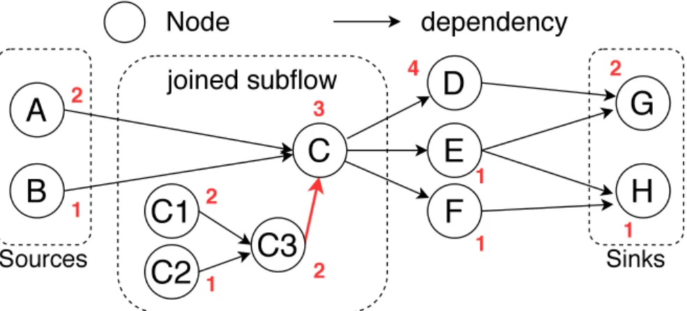
immediately steal the task if there exists one. Figure 2.1 is a task dependency graph with eight tasks (not including the graph spawn by dynamic tasking). Whenever a graph is dispatched to execution, Cpp-Taskflow first creates an object of type tf::Topology to record the runtime data of the graph. The topology object collects the tasks without predecessors (denoted as source tasks, e.g. task A and B) in the task graph, and lets the tasks without successors (denoted as sink tasks, e.g. task G and H) precede a node which

(17)

Figure 2.1: An example to illustrate executing a task dependency graph. The numbers in red are the required execution time of tasks. The red edge is added deliberately by executor to respect the execution order.

will set up the future object at the end of execution. After the topology object has built up, the source tasks are added into the executor’s master queue to initiate the execution. In this example we assume W1 gets task A and W2 gets task B in the beginning. Next we illustrate the task execution along the timeline below:

1. T=1, task B finishes and W2 decrements the dependency of task C. Since W2 has no remaining tasks, W2 will start stealing tasks randomly. 2. T=2, task A finishes and W1 decrements the dependency of task C. Since

task C’s dependency is met, W1 will continue executing task C.

3. T=5, task C finishes and a new task graph is spawned. W1 lets task C3 precede its parent task C. Then, W1 will cache task C1 and add C2 to W1’s local queue. W2 subsequently steals task C2 from W1.

4. T=6, task C2 finishes and W2 decrements the dependency of C3. 5. T=7, task C1 finishes and W1 continues execution on task C3.

6. T=9, task C3 finishes. W1 will revisit task C and decrement the depen-dency of task D, E and F. Task D will be cached by W1 and tasks E and F will be added to W1’s local queue. Then, W2 steals task E from W1’s queue.

7. T=10, task E finishes and W2 decrements the dependency of task G and H. W2 steals task F from W1’s queue.

(18)

8. T=11, task F finishes and W2 decrements the dependency of task H. W2 continues executing task H.

9. T=12, task H finishes. W2 has no tasks in local queue and thus starts random stealing.

10. T=13, task D finishes and W1 decrements the dependency of task G. W1 continues executing task G.

11. T=15, task G finishes. Now all sink nodes are executed and W1 will set up the future object and mark the task graph as finished.

(19)

CHAPTER 3 ADAPTIVE WORK-STEALING

SCHEDULER

3.1 Introduction

Work stealing has been proved to be an efficient approach for parallel task scheduling on multi-core systems and has received wide research interest over the past two decades [11, 13, 14, 15, 16, 17, 18, 19, 20, 21, 22, 23]. Several task-based parallel programming libraries and language have adopted work-stealing scheduler as the runtime for thread management and task dispatch such as Intel Threading Building Blocks (TBB) [9, 24], Cilk [13, 25], X10 [19, 26], Nabbit [27], Microsoft Task Parallel Library (TPL) [28], and Golang [29]. The efficiency of the work-stealing scheduler can be attributed to the way it manages the threads: The scheduler spawns multiple threads (denoted as workers) on initialization. Each worker has a double-ended queue storing the tasks ready for execution, and a worker can only add newly spawned tasks into its queue. A worker first carries out all tasks in its queue, and then becomes a thief to randomly steal tasks from others. When a thief has successfully stolen a task, it restores to a normal worker and commences executing the task. The key is to have thieves actively steal tasks. By doing this the scheduler is able to balance the workload and maximize the performance.

However, implementing an efficient work-stealing scheduler is not an easy job, especially when dealing with a task dependency graph where the par-allelism could be very irregular and unstructured. Due to the decentralized architecture, developers have to sort out many implementation details to ef-ficiently manage workers such as deciding the number of steals attempted by a thief and how to mitigate the resource contention between workers. The problem is even more challenging when considering throughput and en-ergy efficiency, which have emerged as critical issues in modern scheduler

(20)

designs [15] [30]. The worker management can have a huge impact on these issues if it is not designed properly. For example, a straightforward method is to keep workers busy in waiting for tasks. Apparently, this method con-sumes too much resource and can result in a number of problems, such as decreasing the throughput of co-running multithreaded applications and low energy efficiency [15] [30]. Several methods have been proposed to remedy this deficiency, e.g., making thieves relinquish their cores before stealing [16] or backing off a certain time [17] [24], or modifying OS kernel to directly control CPU cores [15]. Nevertheless, these approaches still have drawbacks, especially from the standpoints of solution generality and performance scal-ability.

In this chapter, we propose a work-stealing scheduler with provably good worker management for executing task dependency graphs. Our scheduler employs a simple yet effective strategy that adaptively adjusts the number of thieves by tracking the number of workers that are executing tasks. This strategy has three advantages: First, it ensures one thief will keep looking for tasks when any worker is executing tasks, which can prevent resource from being underutilized. Second, our strategy only uses a reasonable number of workers to meet the parallelism at any time, which can minimize the resource waste without compromising performance. Lastly, this strategy has very little overhead. Workers can quickly carry out their tasks without being slowed down by the extra management work. With this strategy, our scheduler can make efficient use of workers to achieve good performance under different parallelism. Meanwhile, this strategy effectively mitigates the resource waste by reducing unnecessary steals, and therefore our scheduler is energy-efficient and can maintain good throughput when co-running multithreaded processes. We summarize the contributions of our scheduler below:

• An adaptive scheduling strategy: We develop an adaptive scheduling strategy for executing task dependency graph. The strategy is simple; no sophisticated data structures or complex algorithms are required and thus the overhead is small. The experimental results show our scheduler can efficiently utilize CPU resource to achieve good performance.

• Provably good worker management: We proved our scheduler can prevent the under-subscription problem and effectively mitigate the over-subscription problem. Our scheduling algorithm is efficient in balancing

(21)

working threads on top of available task parallelism.

• Energy efficiency: Our scheduler is very energy-efficient in that it re-serves thieves to steal only when there exists a worker executing tasks. We also show that our scheduler will put most thieves put into sleep when tasks are scarce, which effectively reduces resource waste and saves energy. We evaluated the proposed scheduler on two benchmark sets: a set of micro-benchmarks and a very-large-scale integration (VLSI) timing analyzer. We use the Linux utility perf to measure the CPU utilization, runtime and energy usage of ours and the scheduling approach proposed by Aurora et al. [16] (denoted as ABP) and a modified approach from Ding et al. [15]. The micro-benchmarks show our scheduler can utilize the computing resources ef-fectively to accommodate different degrees of parallelism. Specifically, in an extreme case with linear task graph, the CPU utilization of our scheduler is 1.2 while ABP is 31.9, which highlights the effectiveness of our sched-uler’s worker management. The second experiment is a real workload: VLSI static timing analysis. This experiment demonstrates that the scheduler not only achieves scalable performance but is also energy-efficient. On the largest circuit, our scheduler achieves 15% less runtime and 36% less energy consumption than ABP. Finally, we show the scheduler can maintain good throughput when co-running multithreaded applications.

3.2 Adaptive Work-Stealing Scheduler

In this section we present the details of the proposed work-stealing scheduler. We first outline our scheduler’s architecture and associated data structures. Next we describe the proposed worker management approach and its imple-mentation with pseudo code. Lastly, we provide an analysis on our worker management to show its efficiency.

3.2.1 Scheduler Overview

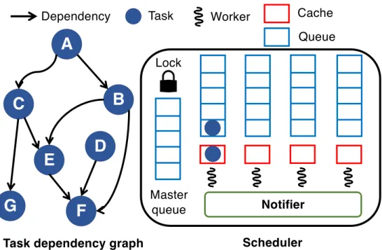
Figure 3.1 shows a task dependency graph (left) and the architecture of the proposed scheduler (right). Our scheduler consists of a set of workers, a master queue, a lock and a notifier. On initialization our scheduler spawns

(22)

A

C

D

B

E

F

G

Dependency Task Master queue Worker Cache Queue Notifier Scheduler Task dependency graph

Lock

Figure 3.1: A task dependency graph and the architecture of our scheduler. workers waiting for tasks. Each worker is equipped with a queue and a cache to store tasks ready for execution. After users create a task graph, they add the source nodes to the master queue and notify workers via the notifier to start execution. Algorithm 2 is the pseudo code of task insertion from users. In Algorithm 2, users first acquire the lock (Algorithm 2 line 1) which prevents concurrent insertion to the master queue. Then users add tasks into the master queue (Algorithm 2 line 2:4) and notify waiting workers (Algorithm 2 line 6). A worker will continue pulling tasks from its queue or others (including the master queue) for execution. When a worker finishes a task, it automatically adds successive tasks ready for execution to its own queue or cache. A worker’s queue allows only the owner to add tasks, while only non-worker threads (such as the main thread controlled by users) can add tasks into the master queue. A cache is simply a task holder and only the owner can access its cache. The cache enables the worker to prefetch a task when the worker adds tasks. For example, in Figure 3.1 a worker can add the task B into its cache and C to its queue after it finishes the task A. With the cache, we can facilitate task retrieval by reducing the queue access.

(23)

Algorithm 2: Task insertion from users

Input: tasks: a set of ready tasks 1 lock();

2 for t in tasksdo

3 master queue.push(t); 4 end

5 unlock();

6 notifier.notify one();

3.2.2 Data Structures

The queue and the notifier are two important data structures in our scheduler. We implement the queues (both the worker’s queue and master queue) based on the Chase-Lev algorithm [12] [31]. Access to the queue is non-blocking and the queue capacity can grow if more space is needed. The queue provides three operations:

1. Push: Add a task into the bottom of the queue. Only the queue’s owner can use this operation.

2. Pop: Retrieve a task from the bottom of the queue. Only the queue’s owner can use this operation.

3. Steal: Retrieve a task from the top of the queue. Any worker can use this operation.

Thenotifieris a synchronization component that is capable of (1) putting workers that are waiting for tasks into sleep and (2) notifying one or all wait-ing workers when new tasks are present or the scheduler terminates. In our scheduler, we use the EventCount struct from the Eigen library [32] as the

notifier. The usage of EventCount is similar to a condition variable. The notifying thread sets a condition to true and then signals waiting workers via EventCount. On the other side, a worker first checks the condition and returns to work if the condition is true. Otherwise, the worker updates the

EventCount to indicate it is waiting and checks the condition again. If the condition is still false, the worker is put into sleep via the EventCount.

(24)

3.2.3 Worker Management

Recall that our scheduler spawns workers on initialization and Algorithm 3 contains the pseudo code for spawning workers and a worker’s control flow. In the spawn function, the scheduler spawnsN workers where N is specified by users. The scheduler makes workers execute the worker loop function after they are spawned. The worker loop function consists of two steps. In the first step exploit task, a worker executes a ready task and the tasks in its queue (Algorithm 3: line 10) until its queue becomes empty. Next, the worker leaves the exploit task and calls the wait for task (Algorithm 3: line 11) to start stealing tasks. If the worker successfully steals a task, it returns from the wait for task and repeats the first step. Otherwise, the worker is put into sleep via the notifier to wait for task notification. When the scheduler terminates, the wait for task returns false and the worker exits the while-loop.

Algorithm 3: spawn

Input: N: number of workers 1 Function spawn(N):

2 for i←0 to N do

3 workers.emplace back(worker loop(i));

4 end

5 ;

6 Function worker loop(id): 7 w ←workers[id];

8 t ← NIL; 9 while true do

10 exploit task(t, w);

11 if wait for task(t, w) == false then

12 break;

13 end

14 end 15 return

One major contribution of this work is the adaptive scheduling algorithm, which is implemented in the exploit task and wait for task functions. The main idea of this algorithm is to maintain at least one thief (except when all workers are executing tasks) when a worker is executing tasks. This is different from prior research where they unconditionally keep one or more thieves busy in waiting tasks [15][16], whereas we keep thieves only when

(25)

there exists potential parallelism. We achieve this by using two counters:

num actives and num thieves to adaptively adjust the number of thieves. Algorithm 4 is the pseudo code ofexploit taskfunction. In this function, the worker first increments thenum actives(Algorithm 4: line 2) and checks the num thieves (Algorithm 4: line 2). If num thieves is zero and this is the first increment on num actives, then the worker notifies a waiting worker (Algorithm 4: line 3) and proceeds to execute the task. The worker continues fetching and executing tasks from its cache (Algorithm 4: line 8) and queue (Algorithm 4: line 10) until both become empty. Then the worker decrements the num actives (Algorithm 4: line 13) and returns. Obviously, the num actives records the number of workers that are executing tasks, and a non-zero num actives implies there could be tasks in a queue.

After a worker returns fromexploit task, the worker starts stealing tasks by invoking the wait for task function. Algorithm 5 is the pseudo code of thewait for taskfunction. In thewait for task, the thief first increments the num thieves (Algorithm 5: line 2) and conducts random stealing by invoking the explore task function (Algorithm 5: line 4). Algorithm 6 is the pseudo code of the explore task function. In the explore task, the thief first randomly selects a victim (Algorithm 6: line 4) which could be other workers or the master queue. Then it tries to steal a task from the victim (Algorithm 6: line 5:9). If the steal fails, the thief will attempt to steal for a certain number of times. When the number of failed steals is greater than a pre-defined threshold, steal bound (Algorithm 6: line 14), the thief invokes a yield system call every time after each failed steal. A thief stops stealing if it still cannot obtain any task after yielding yield bound times (Algorithm 6: line 17). The thief returns from explore task in either one of the three conditions:

• The thief successfully steals a task (Algorithm 6: line 11). • The scheduler terminates (Algorithm 6: line 3),

• The thief fails to obtain any task after a fixed number of attempts (Algo-rithm 6: line 18).

In the first case, the thief decrements num thieves (Algorithm 5: line 5) and notifies a waiting worker if it is the last thief (Algorithm 5: line 6). For the other two cases, the thief first updates the notifier (Algorithm 5: line

(26)

10) to indicate it is waiting. Next the thief checks the master queue and tries to steal a task if the queue is non-empty (Algorithm 5: line 11:22). The thief returns (Algorithm 5: line 18) if it successfully steals a task from the master queue or goes back to steal tasks if it failed (Algorithm 5: line 20). Otherwise, the thief proceeds to check the scheduler’s status. If the scheduler shuts downs (Algorithm 5: line 23), the thief notifies all waiting workers (Algorithm 5: line 25) and then decrements the num thieves and returns. If all preceding conditions do not hold, the thief decrements the

num thieves and then either continues to steal if num actives is non-zero (Algorithm 5: line 31) and it is the last thief, or goes into sleep (Algorithm 5: line 33).

Algorithm 4: exploit task

Input: t: a task holder,w: the worker’s data structure 1 if t6=NIL then

2 if AtomInc(num actives) == 1 and num thieves == 0 then 3 notifier.notify one();

4 end

5 do

6 execute(t);

7 if w.cache6=NIL then

8 t ←w.cache;

9 else

10 t ←pop(w.queue);

11 end

12 while t6=NIL;

13 AtomDec(num actives); 14 end

3.2.4 Analysis

We show the scheduler’s worker management is very efficient in two fronts: (1) At least one thief exists when there is a worker executing tasks. (2) It mitigates the thieves over-subscription problem by putting most thieves into sleep after they failed to steal. We first define the states of a worker:

Definition A worker is active if it is exploiting tasks (Algorithm 4: line 2:13), otherwise, the worker is inactive.

(27)

Algorithm 5: wait for task

Input: t: a task,w: the worker’s data structure

Output: A Boolean value to indicate continuation of worker-loop

1 wait for task:

2 AtomInc(num thieves);

3 explore task:

4 if explore task(t, w) and t6=NILthen 5 if AtomDec(num thieves) == 0 then 6 notifier.notify one();

7 end

8 returntrue; 9 end

10 notifier.prepare wait(w);

11 if master queue is not empty then 12 notifier.cancel wait(w);

13 t← steal(master queue); 14 if t6=NIL then

15 if AtomDec(num thieves) == 0 then 16 notifier.notify one(); 17 end 18 return true; 19 else 20 go to explore task; 21 end 22 end

23 if scheduler stops then 24 notifier.cancel wait(w); 25 notifier.notify all(); 26 AtomDec(num thieves); 27 returnfalse;

28 end

29 if AtomDec(num thieves) == 0 and num actives > 0 then 30 notifier.cancel wait(w);

31 go towait for task; 32 end

33 notifier.commit wait(w); 34 returntrue;

Definition An inactive worker is sleeping if it has been suspended by the notifier (Algorithm 5: line 33).

(28)

(Algo-Algorithm 6: explore task

Input: t: a task holder,w: the worker’s data structure

Output: t

1 num f ailed steals← 0; 2 num yields← 0;

3 while scheduler not stops do 4 victim ← random(); 5 if victim == w then

6 t ←steal(master queue); 7 else

8 t ←steal task from(victim);

9 end

10 if t6=NIL then

11 break;

12 else

13 num f ailed steals ←num f ailed steals+ 1; 14 if num f ailed steals≥steal boundthen

15 yield();

16 num yields ←num yields + 1; 17 if num yields== yield bound then

18 break;

19 end

20 end

21 end 22 end

rithm 4: line 2:13) nor sleeping.

Lemma 1. When a worker is active and at least one worker is inactive, one thief always exists.

Proof. Assume there exists one active worker and one inactive worker. The inactive worker is either awake (Algorithm 5: line 1:28) or sleeping (Algo-rithm 5: line 33). If the inactive worker is awake, then it is a thief and the lemma holds. Otherwise the inactive worker is sleeping and it must have decremented the num thieveswithout seeing any active worker (Algo-rithm 5: line 29). This happens only when the active worker just enters the

exploit taskfunction and is about to incrementnum actives(Algorithm 4: line 2). Subsequently the active worker shall wake up a thief (Algorithm 4: line 3) and the lemma holds.

(29)

Lemma 1 is important to our scheduler as it prevents theunder-subscription problem.

Definition An under-subscription problem means: T = 0 and 0< Q < W where

Q: number of non-empty queues (excluding the master queue) T : number of thieves

W : number of total workers

In the following discussion we exclude two special conditions where all workers are active and all workers are inactive. An under-subscription prob-lem occurs when all thieves go into sleep (i.e. T = 0) while at least one queue is non-empty. The under-subscription problem degrades the sched-uler’s performance since the scheduler does not fully exploit the available parallelism. With Lemma 1, we show that our scheduler does not have the under-subscription problem:

Lemma 2. Our work-stealing scheduler always has 0< T if 0< Q < W

Proof. In our scheduler a worker is active if its queue is non-empty (Algo-rithm 4):

Q≤A

where A is the number of active workers, and by Lemma 1: T ≥1 if 0< A < W

Combining these two inequalities, we have:

(30)

Lemma 2 guarantees at least one thief exists when there is a non-empty queue, which prevents the under-subscription problem. Lemma 2 also enables us to offload the task notification from active workers to thieves. In our scheduler workers do not need to notify waiting workers when spawning new tasks. Instead, a thief will notify a waiting worker when the steal succeeds and it is the last thief that decrements the num thieves (Algorithm 5: line 5:6). This allows active workers to quickly add new tasks without being stalled by the notification.

Our scheduling method not only prevents the under-subscription problem but can also mitigate the over-subscription problem. The over-subscription problem means the number of thieves is greater than the number of available tasks. Mitigating the over-subscription problem is very important for two reasons: First, excessive thieves will cause substantial resource wasted on failed steals if they persist for a long time. Second, excessive thieves and active workers might contend for resource, which can result in inefficient resource utilization. We now show the scheduler will put most thieves into sleep within a time bound if they fail to steal any task.

Definition Assume there exists more than one thief. We call these thieves a group and a thief leaves the group if it goes into sleep (Algorithm 5: line 33) or successfully steals a task (Algorithm 6: line 10).

Given a group, we prove that only one thief exists in the group after a certain time. This implies most thieves will go into sleep when there are no sufficient tasks. In the following proof, we assume the master queue is empty since thieves will check the master queue before going to sleep. For better description, we denote the constants steal bound and yield bound

in Algorithm 6 as α and β, respectively.

Lemma 3. Given a group of thieves, only one thief in the group exists after O((α+β)∗S+C) time, where S is the time to perform a steal and C is a constant.

Proof. Given a group of thieves, we call the thief that lastly decrements the num thieves (Algorithm 5: line 5 and 29) in this group as thelast thief. Thieves in a group except the last thief must either (1) become active workers if they successfully steal tasks (Algorithm 5: line 4) or (2) go into sleep (Algorithm 5: line 33) after they decrement the num thieves. Therefore,

(31)

eventually only one thief stays in the group when the last thief performs the decrement. Next we analyze the runtime taken by the last thief to do the decrement. There are two cases: the last thief either successfully steals a task (Algorithm 5: line 4) or fails to steal any task (Algorithm 5: line 29). For the first case, the runtime is bounded by O((α+β)∗S) where S is the time of conducting one steal and (α+β) is the maximum number of steals that can be attempted. For the second case, the last thief will go through following steps:

1. Perform (α+β) steals (Algorithm 5: line 4). 2. Prepare for sleep (Algorithm 5: line 10).

3. Check the master queue (Algorithm 5: line 11) and the scheduler status (Algorithm 5: line 23).

Because steps 2 and 3 are simple routines, we use a constant C to denote the maximal total runtime took by these two steps. Then the runtime of the second case is bounded by O((α+β)∗S+C). Therefore, the runtime for the last thief to perform the decrement will be bounded byO((α+β)∗S+C).

To sum up, we proved our scheduler can prevent the under-subscription problem (Lemma 2) and effectively mitigate the over-subscription problem (Lemma 3). Our scheduling algorithm is simple and efficient in balancing working threads on top of available task parallelism. We will demonstrate the practical performance in the experiment results.

3.3 Evaluation

We evaluated our scheduler using a set of micro-benchmarks and a timing analyzer for VLSI systems. We compare our scheduler with two approaches: the ABP method [16], and the MBWS which is modified from the BWS of Ding et al. [15]. For fair comparison, we implement all scheduling methods in Cpp-Taskflow. We briefly summarize our implementation of ABP and MBWS: ABP lets thieves repeatedly steal until they succeed, and thieves will invokeyieldsystem call every time before attempting a steal. BWS [15] introduces two methods to enhance ABP’s resource utilization: (1) BWS modifies the OS kernel so that workers can query the running status of others

(32)

and yield their cores directly to others. (2) BWS uses two counters, a wake-up and a steal counter, to make thieves wake wake-up two sleeping workers for busy workers and limit the number of steals a thief can attempt. We modify BWS as follows: First, we do not modify the OS kernel as we aim for a portable solution that does not introduce system-specific hard code. To compensate for this, we associate each worker with a status flag which is set by the owner to inform its current status, and thieves do not yield their cores. Second, we implement the modified counter-based approach in the

explore task function. As multiple thieves can concurrently modify the wake-up counter, we use atomic compare-and-swap operation to decrement the wake-up counter. A deficiency of BWS is that all thieves could be sleeping while the parallelism changes. To resolve this problem, BWS has to keep one watchdog worker which never goes into sleep to prevent missing parallelism. We also implemented this mechanism in MBWS by having a thief continue to steal if it is the last one that decrements the num thieves. Notice that the modified BWS may not be reflective of the true implementation but it provides a good reference to implement the wake-up-two heuristic.

We conducted all experiments on a machine with two Intel Xeon Gold 6138 processors (2 NUMA nodes) and 256 GB memory. Each processor has 20 cores with 2 threads per core. The OS is Ubuntu 19.04 and the compiler is GCC 8.3.0. We compile all source code with the optimization flag O2

and C++ 17 standard flag (-std=c++17). To reduce the impact of thread migration, we use the system command taskset to bond the threads to a set of cores, and we split the threads evenly on the two processors. The

steal bound is set to 2∗(number of workers + 1) and the yield bound is 100. For MBWS we adopt 64 as the SleepThreshold, which is the same as the experiment setting in [15]. We report the results measured by Linux profiling utility perf.

3.3.1 Micro-benchmarks

We select four micro-benchmarks with different kinds of parallelism. This experiment is to provide insight into the schedulers’ CPU utilization under various task dependency graphs.

(33)

one successor and one predecessor except the first and last tasks. Each task increments a counter by 1. The size of the graph is 8388608.

• Binary tree: The task graph is a binary tree, i.e. each task has one prede-cessor and two sucprede-cessors except the root and leaf tasks. The task has no computation. The size of the graph is 8388607.

• Graph traversal: We generate a task graph where the dependency is ran-domly determined, and the number of successors of a node is bounded by a given value. Each task sets a Boolean variable to true to indicate the associated node is visited. The size of the graph is 4000000.

• Matrix multiplication: Given three matrices (2-D array with size 2048x2048), we create a task graph to perform the matrix multiplication. The task graph has two levels: (1) In the first level each task initializes the elements in a row of a matrix. (2) In the second level each task computes a row in the resulting matrix. Tasks in the same level are independent of each other and we create an empty task to synchronize the first level before starting the second level.

In this experiment, we vary the number of cores among 1, 4, 8, 12, 16, 20, 24, 28, 32, 36 and 40. We first compare the schedulers’ performance and CPU utilization in all four cases. Then we vary the task granularity of two benchmarks with irregular and regular dependency to observe their performance, CPU utilization and energy consumptions. For each scheduler we report the average value of ten runs on each benchmark (the command is

perf stat -r).

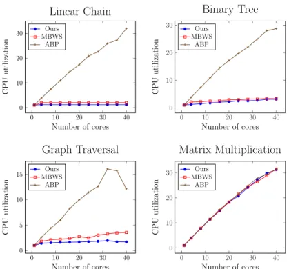
Figures 3.2 and 3.3 show the runtime and CPU utilization of each bench-mark, respectively. For the linear chain, the runtime does not decrease when adding more cores. This is expected as the linear chain has no parallelism at all and one core should suffice for the execution. The CPU utilization of ABP increases along with the number of cores while both MBWS and ours remain nearly uninfluenced. In fact, the CPU utilizations of MBWS and ours stay around 2.0 and 1.2 from 4 to 40 cores respectively.

(34)

0 10 20 30 40 3 4 5 6 7 8 Number of cores R u n ti m e (s ) Linear Chain Ours MBWS ABP 0 10 20 30 40 3 4 5 6 Number of cores R u n ti m e (s ) Binary Tree Ours MBWS ABP 0 10 20 30 40 3 3.5 4 4.5 5 5.5 Number of cores R u n ti m e (s ) Graph Traversal Ours MBWS ABP 0 10 20 30 40 0 10 20 30 40 Number of cores R u n ti m e (s ) Matrix Multiplication Ours MBWS ABP

Figure 3.2: Runtime comparisons between ours, MBWS, and ABP on micro-benchmarks. 0 10 20 30 40 0 10 20 30 Number of cores C P U u ti li za ti on Linear Chain Ours MBWS ABP 0 10 20 30 40 0 10 20 30 Number of cores C P U u ti li za ti on Binary Tree Ours MBWS ABP 0 10 20 30 40 0 5 10 15 Number of cores C P U u ti li za ti on Graph Traversal Ours MBWS ABP 0 10 20 30 40 0 10 20 30 Number of cores C P U u ti li za ti on Matrix Multiplication Ours MBWS ABP

Figure 3.3: CPU utilization comparisons between ours, MBWS, and ABP on micro-benchmarks.

(35)

0 10 20 30 40 4 6 8 Number of cores R u n ti m e (s )

0.5M iterations per task

Ours MBWS ABP 0 10 20 30 40 4 6 8 10 12 Number of cores R u n ti m e (s )

1M iterations per task

Ours MBWS ABP 0 10 20 30 40 5 10 15 Number of cores R u n ti m e (s )

Ours MBWS ABP 0 10 20 30 40 5 10 15 20 Number of cores R u n ti m e (s )

Ours MBWS

ABP

Figure 3.4: Runtime comparisons between different task granularities (number of iterations). 0 10 20 30 40 0 5 10 15 Number of cores C P U u ti li za ti on

Ours MBWS ABP 0 10 20 30 40 0 5 10 15 20 Number of cores C P U u ti li za ti on

Ours MBWS ABP 0 10 20 30 40 0 5 10 15 Number of cores C P U u ti li za ti on

Ours MBWS ABP 0 10 20 30 40 0 5 10 15 20 Number of cores C P U u ti li za ti on

Ours MBWS

ABP

Figure 3.5: CPU utilization comparisons between different task granularities (number of iterations).

(36)

0 10 20 30 40 0 10 20 30 40 Number of cores R u n ti m e (s )

4 rows per task

8 rows per task

16 rows per task

32 rows per task

Ours MBWS

ABP

Figure 3.6: Runtime comparisons between different task granularities (number of rows per task).

0 10 20 30 40 0 10 20 30 Number of cores C P U u ti li za ti on

4 rows per task

8 rows per task

16 rows per task

32 rows per task

Ours MBWS

ABP

Figure 3.7: CPU utilization comparisons between different task granularities (number of rows per task).

(37)

1 4 8 12 16 20 24 28 32 36 40 0 1,000 2,000 3,000 4,000 Number of cores E n er gy u sa ge (J ou le )

4 rows per task

Ours MBWS ABP 1 4 8 12 16 20 24 28 32 36 40 0 1,000 2,000 3,000 4,000 Number of cores E n er gy u sa ge (J ou le )

8 rows per task

16 rows per task

32 rows per task

Ours MBWS

ABP

Figure 3.8: Energy usage of ours, MBWS, and ABP on matrix multiplication with different numbers of rows per task.

This example shows that although a thief can possibly yield its core to other workers before stealing, keeping thieves awake can still incur high CPU utilization. For the binary tree and graph traversal, the runtimes of all schedulers drop to a stable point after 4 cores. Adding more cores does not improve the performance as the workload of their tasks is very small and a worker might quickly carry out all tasks in its queue before thieves discover them. ABP has the highest CPU utilization among all schedulers and ours is the lowest in both cases. The CPU utilization of ABP also grows more rapidly than others in these two cases.

For the matrix multiplication, which has better scalability than the pre-vious three cases, the runtimes of all schedulers are very close and their CPU utilizations exhibit similar growth trends. There are two main reasons accounting for this: (1) In the matrix multiplication, intra-level tasks are independent of each other and those tasks have nearly equal workload. (2) The multiplication is compute-intensive and thus the runtime is dominated

(38)

12 16 20 24 28 32 36 40 0 200 400 600 800 Number of cores E n er gy u sa ge (J ou le )

16 rows per task

Ours MBWS ABP 12 16 20 24 28 32 36 40 0 200 400 600 800 Number of cores E n er gy u sa ge (J ou le )

32 rows per task

Ours MBWS

ABP

Figure 3.9: Energy usage of ours, MBWS, and ABP on matrix multiplication with 16 and 32 rows per task.

by the computation rather than the scheduling overhead.

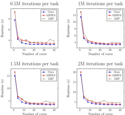
Next, we further evaluate these schedulers by tuning the task granularity. In this experiment we select two benchmarks: graph traversal and matrix multiplication, The former has irregular dependency between tasks, while in the latter tasks in the same layer are independent. For each task in the graph traversal benchmark, we deliberately add a for-loop which iteratively performs division, and we change the loop’s number of iterations to adjust the tasks’ workload. The numbers of iterations tested in this experiment are 5 × 105

, 1 ×106

, 1.5× 106

and 2 ×106

. Figure 3.4 and 3.5 are the runtime and CPU utilization of all schedulers under different numbers of iterations, respectively. In general, in all scenarios adding more cores can improve all schedulers’ performance. The CPU utilizations of all schedulers increase along with the number of iterations. The reason for this could be that with more iterations a worker will take longer to execute a single task, and this will give more time for the idle workers to steal tasks. We observe that ABP has a noticeable fluctuation in CPU utilization, while the CPU utilizations of ours and MBWS increase steadily. Under the same number of iterations, ABP has the highest CPU utilization; nevertheless the runtime of ABP is higher than others. On the contrary, our scheduler can get better performance than both ABP and MBWS with less CPU utilization.

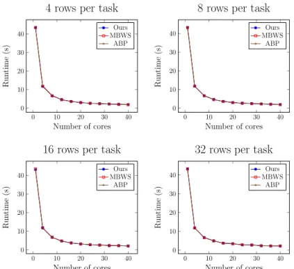
Finally for the matrix multiplication benchmark, we delegate the compu-tations of multiple rows in the resulting matrix to each task to vary the work-load. Figure 3.6 and 3.7 are the runtime and CPU utilization of all schedulers under different numbers of rows, respectively. Regarding the performance, all

(39)

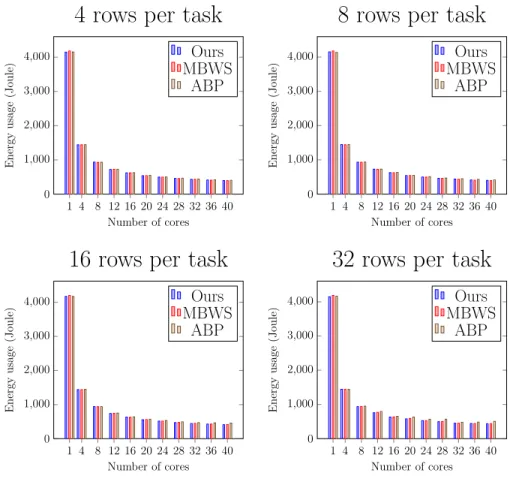
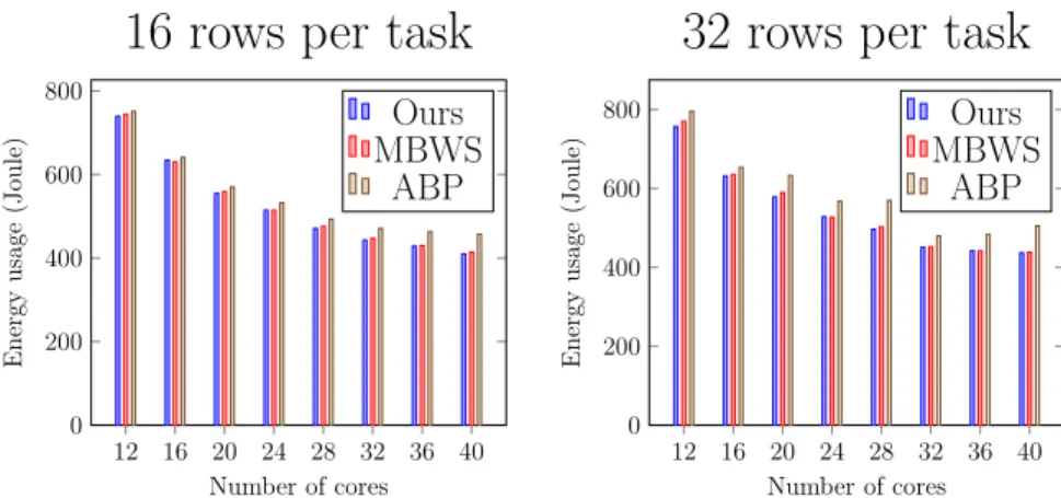
schedulers have very similar runtime and scalability in all workloads. For the CPU utilization, we found that ABP has higher CPU utilization when a task is given more rows, especially when the number of available cores increases. Because the total number of tasks is inversely proportional to the number of rows in a task, this result shows that ABP can cause excessive CPU usage when there is no sufficient task. Over-subscription of the CPU resource can lead to inefficient energy use which is shown in Figure 3.8. To clearly demon-strate the difference, we specifically single out the energy consumptions of 16 and 32 rows with using more than 8 cores in Figure 3.9, which shows that ABP consumes more energy than the others. For instance, ABP consumes 13.2% and 13.5% more energy than MBWS and ours respectively, when there are 40 cores and a task is assigned 32 rows.

To conclude, our scheduler can deliver comparable performance to others under various task dependency graphs and is more efficient in CPU utiliza-tion. The latter can contribute a lot to the energy efficiency and throughput of co-running multithreaded applications, which will be demonstrated later in a large-scale workload.

3.3.2 VLSI Timing Analysis

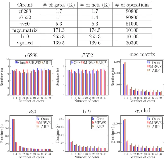
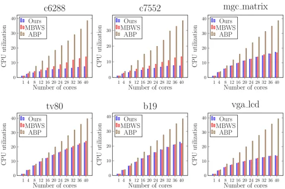
Next we evaluate the schedulers on a real-world application: VLSI timing analyzer. Static timing analysis (STA) plays a critical role in the circuit design flow. For a circuit to function correctly, its timing behavior must meet all requirements under different design constraints and environment settings. Thus, circuit designers have to apply STA to verify the circuit’s timing behavior during different stages in the design flow. STA calculates the timing-related information by propagating through the gates in a circuit, and this workload can be naturally described using a task dependency graph. In this experiment, we use these schedulers to execute the task graph built in OpenTimer [7], an open-source VLSI timer. We randomly generate a set of operations which incrementally modify a given circuit and then perform STA to update the timing. We use the circuits from TAU 2015 timing contest [33] and the statistics of the circuits are listed in Table 3.1. For each circuit we ran OpenTimer five times and report the average runtime and CPU utilization recorded byperf. Figure 3.10 and 3.11 show the runtime and CPU utilization

(40)

Table 3.1: Statistics of circuits

Circuit # of gates (K) # of nets (K) # of operations

c6288 1.7 1.7 80800 c7552 1.1 1.4 80800 tv80 5.3 5.3 51000 mgc matrix 171.3 174.5 10100 b19 255.3 255.3 10100 vga lcd 139.5 139.6 30300 1 4 8 12 16 20 24 28 32 36 40 0 2 4 6 8 10 Number of cores R u nt im e (s )

c6288

Ours MBWS ABP 1 4 8 12 16 20 24 28 32 36 40 0 2 4 6 Number of cores R u nt im e (s )

c7552

Ours MBWS ABP 1 4 8 12 16 20 24 28 32 36 40 500 1,000 1,500 Number of cores R u nt im e (s )

mgc matrix

Ours MBWS ABP 1 4 8 12 16 20 24 28 32 36 40 0 200 400 600 800 Number of cores R u nt im e (s )

tv80

Ours MBWS ABP 1 4 8 12 16 20 24 28 32 36 40 0 1,000 2,000 3,000 4,000 Number of cores R u nt im e (s )

b19

Ours MBWS ABP 1 4 8 12 16 20 24 28 32 36 40 0 1,000 2,000 3,000 Number of cores R u nt im e (s )

vga lcd

Ours MBWS ABP

Figure 3.10: Runtime comparisons between ours, MBWS, and ABP on OpenTimer.

of each circuit respectively.

We categorize the circuits into different groups based on their sizes and discuss the results. For those small circuits c6288 and c7552, their runtimes do not scale with the number of cores. The CPU utilizations of all schedulers on these two circuits increase along with the number of cores, and ABP has the highest CPU utilization followed by the MBWS and ours is the smallest. Next for the medium size circuit tv80, the runtimes of all schedulers decrease after adding more cores. ABP is faster than others except at single core and the runtimes at 40 cores are 60.4 (ours), 60.8 (MBWS) and 52.5 (ABP), respectively. We attribute this to the overhead of notifying workers. Both

(41)

1 4 8 12 16 20 24 28 32 36 40 0 10 20 30 40 Number of cores C P U u ti li za ti on

c6288

Ours MBWS ABP 1 4 8 12 16 20 24 28 32 36 40 0 10 20 30 Number of cores C P U u ti li za ti on

c7552

Ours MBWS ABP 1 4 8 12 16 20 24 28 32 36 40 0 10 20 30 40 Number of cores C P U u ti li za ti on

mgc matrix

tv80

b19

vga lcd

Ours MBWS ABP

Figure 3.11: CPU utilization comparisons between ours, MBWS, and ABP on OpenTimer.

ours and MBWS will put thieves into sleep and notify them when tasks present, while in ABP all thieves are kept busy in waiting for tasks. In terms of the CPU utilization, ABP is still the highest and ours and MBWS are very close. Lastly, for those large circuits with over 100,000 gates: mgc matrix, b19, and vga lcd, the performance scales with the number of cores in all schedulers. When using multiple cores, ABP is slower than others even though ABP’s CPU utilization remains the highest. Take the largest circuit b19 with 40 cores as an example; the runtime of ours is 5% and 15% less than MBWS and ABP, respectively, and the CPU utilizations are 22.7 (ours), 21.7 (MBWS) and 38.5 (ABP). This experiment shows that our scheduler has competitive performance, and can utilize the CPU resource in a reasonable way under a large-scale workload.

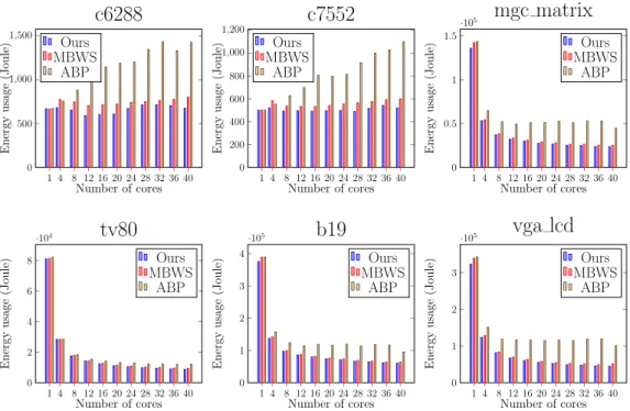
Next we demonstrate the energy usage and power consumption of each scheduler with OpenTimer. Intel has provided users the Running Average Power Limit (RAPL) [34] interface for power management on recent proces-sors. We use perf, which can access the RAPL interface, to measure the energy consumed by two packages (2 NUMA nodes) during the execution (the command is perf stat -e power/energy-pkg/ -a), and we let perf

(42)

1 4 8 12 16 20 24 28 32 36 40 0 500 1,000 1,500 Number of cores E n er gy u sa ge (J ou le)

c6288

Ours MBWS ABP 1 4 8 12 16 20 24 28 32 36 40 0 200 400 600 800 1,000 1,200 Number of cores E n er gy u sa ge (J ou le)

c7552

Ours MBWS ABP 1 4 8 12 16 20 24 28 32 36 40 0 0.5 1 1.5 ·105 Number of cores E n er gy u sa ge (J ou le)

mgc matrix

Ours MBWS ABP 1 4 8 12 16 20 24 28 32 36 40 0 2 4 6 8 ·104 Number of cores E n er gy u sa ge (J ou le)

tv80

Ours MBWS ABP 1 4 8 12 16 20 24 28 32 36 40 0 1 2 3 4 ·105 Number of cores E n er gy u sa ge (J ou le)

b19

Ours MBWS ABP 1 4 8 12 16 20 24 28 32 36 40 0 1 2 3 ·105 Number of cores E n er gy u sa ge (J ou le)

vga lcd

Ours MBWS ABP

Figure 3.12: Energy usage of ours, MBWS, and ABP on OpenTimer. report the average value of five runs.

Figure 3.12 is the average energy usage reported byperf, and we divide the energy usage by the runtime to derive the power consumption which is shown in Figure 3.13. For energy usage, ABP is the highest in all cases. MBWS is very close to ours with ours performing slightly better in most cases. For small circuits like c6288 and c7552, the energy usage of ABP increases along with the number of cores even the performance does not scale. For example, in c6288 the energy usage of ABP is 2x of ours at 40 cores but the runtime of ABP is only 8% less than ours. For other circuits, the energy usage of all schedulers decreases after adding more cores as those circuits have good scalability. However, ABP’s energy usage is still much higher than others. For example, in the largest circuit b19 ABP’s energy usage is 1.57x of ours and 1.48x of MBWS when using 40 cores. Next for the power consumption, ABP’s power consumption increases along with the core numbers in all cases. The result shows that thieves can still consume substantial power even mak-ing them yield frequently. This is especially evident in small circuits c6288 and c7552 where ABP’s power consumption doubles when the number of cores increases from 1 to 40. In contrast, the power consumptions of ours and MBWS do not show substantial growth after adding more cores in these

(43)

1 4 8 12 16 20 24 28 32 36 40 0 50 100 150 200 250 Number of cores P ow er co n su m p ti on

c6288

Ours MBWS ABP 1 4 8 12 16 20 24 28 32 36 40 0 50 100 150 200 250 Number of cores P ow er co n su m p ti on

c7552

mgc matrix

tv80

b19

vga lcd

Ours MBWS ABP

Figure 3.13: Power consumption (energy/runtime) of ours, MBWS, and ABP on OpenTimer.

two circuits. For larger circuits, the power consumption of all schedulers increases along with the core numbers, and again ABP’s grows faster than others. In the largest circuit b19 with 40 cores, the power consumptions of ours and MBWS are 26% and 25% less than ABP, respectively.

In the last experiment, we measure the effect of co-running multiple Open-Timers. This experiment is to simulate real working environment which is typically shared by multiple users such as servers or cloud computing plat-forms. In those environments users can run multithreaded applications con-currently, and applications might request computing resources more than their actual parallelism.

In this experiment, we run multiple OpenTimers simultaneously on the same circuit and every timer can use all the cores (40 on our machine). The number of OpenTimers in the co-runs ranges from 2 to 8 and we use the

time command to measure the runtime (wall clock time) of each timer. We repeat each co-run five times and use the average as the throughput. For each scheduler, we take the runtime of its solo-run as the baseline and compute the throughput using the speedup method [15] [35]. The weighted-speedup method sums the weighted-speedup of each process in the co-runs, where the

(44)

2 3 4 5 6 7 8 0

2 4 6

Number of co-run timers

T h ro u gh p u t

c6288

Ours MBWS ABP 2 3 4 5 6 7 8 0 2 4 6

T h ro u gh p u t

c7552

Ours MBWS ABP 2 3 4 5 6 7 8 0 1 2 3

T h ro u gh p u t

mgc matrix

Ours MBWS ABP 2 3 4 5 6 7 8 0 1 2 3

T h ro u gh p u t

tv80

Ours MBWS ABP 2 3 4 5 6 7 8 0 0.5 1 1.5 2 2.5

T h ro u gh p u t

b19

Ours MBWS ABP 2 3 4 5 6 7 8 0 1 2 3 4

T h ro u gh p u t

vga lcd

Ours MBWS ABP

Figure 3.14: Throughput comparisons of co-running multiple OpenTimers. speedup is defined asTbaseline/Tper proc. Figure 3.14 shows the throughputs of all schedulers on different circuits. ABP has the lowest throughput in all co-runs regardless the circuit size. For example, when co-running 8 OpenTimers, the throughputs of ABP are 1.49 and 2.74 on b19 and c7552, respectively, while ours is 1.89 and 5.9 and MBWS is 1.95 and 4.2. MBWS and ours have similar throughput except at c6288 and c7552 where ours is much higher.

3.4 Conclusion

In this chapter, we have introduced a work-stealing scheduler for executing task dependency graph. We have designed an efficient worker management method that adaptively adjusts the number of thieves by tracking the number of workers that are executing tasks. This method not only effectively prevents resource from being underutilized but also mitigates resource waste. We have evaluated the scheduler on a set of micro-benchmarks and a VLSI timing analyzer. The results show our scheduler achieved comparable performance to existing approaches, with effective resource utilization and good energy efficiency.

(45)

CHAPTER 4 TASK GRAPH COMPOSITION AND

CONDITIONALS

4.1 Introduction

The key to make developers productive in writing software is composability. We use libraries written by other developers to compose a large program, or we decompose a job into smaller pieces to tame the complexity in soft-ware development. Composability is especially important in developing fast market-expanding applications such as high-performance machine learning, data analytics, and parallel simulation engines [36]. These applications ex-hibit both regular and irregular compute patterns, and are often combined with other functions to compose large software that will be deployed on a multicore machine or a distributed cloud [37, 38]. However, composable paral-lel processing is rarely addressed as the first-class concept by existing parallel programming libraries [39]. Many libraries were designed to solve a single hard problem as fast as possible, leaving users to decide composition with their own practice. This can create a lot of pain and data engineering tasks for developers of different teams to collaborate on a large parallel application. Some common problems include confusing API mix-uses, unwanted coupling layers, error-prone dependency wrappers, inconsistent threading models, and suboptimal scheduling results.

The traditional interface for program decomposition is function call. De-velopers break down a large sequential program into a specific set of tasks each wrapped in a function call with clear definition of data exchange. These function calls are often modular and reusable to make the codebase main-tainable and readable. However, composable parallel programming is much more challenging. Modern parallel workloads typically combine a broad mix of algorithms, functions, and libraries. Each library manages its own threads and task execution, making it difficult to perform optimization across

Advances in parallel programming for electronic design automation

ABSTRACT

ACKNOWLEDGMENTS

TABLE OF CONTENTS

CHAPTER 1

DISSERTATION OVERVIEW

CHAPTER 2

CPP-TASKFLOW PROGRAMMING

SYSTEM

2.1 Task Dependency Graph

2.2 Software Architecture and Execution Flow

CHAPTER 3

ADAPTIVE WORK-STEALING

SCHEDULER

3.1 Introduction

3.2 Adaptive Work-Stealing Scheduler

3.2.1 Scheduler Overview

A

C

D

B

E

F

G

3.2.2 Data Structures

3.2.3 Worker Management

3.2.4 Analysis

3.3 Evaluation

3.3.1 Micro-benchmarks

4 rows per task

8 rows per task

16 rows per task

32 rows per task

16 rows per task

32 rows per task

3.3.2 VLSI Timing Analysis

c6288

c7552

mgc matrix

tv80

b19

vga lcd

c6288

c7552

mgc matrix

tv80

b19

vga lcd

c6288

c7552

mgc matrix

tv80

b19

vga lcd

c6288

c7552

mgc matrix

tv80

b19

vga lcd

c6288

c7552

mgc matrix

tv80

b19

vga lcd

3.4 Conclusion

CHAPTER 4

TASK GRAPH COMPOSITION AND

CONDITIONALS

4.1 Introduction