CENTRE D’ETUDES ET DE RECHERCHES SUR LE DEVELOPPEMENT INTERNATIONAL
Document de travail de la série Etudes et Documents
Ec 2001.06
Does the Balassa-Samuelson effect apply to the Chinese provinces?
by
Sylviane GUILLAUMONT JEANNENEY*
and Ping HUAa*
CERDI-IDREC, CNRS-Université d’Auvergne
October 2001, 35 p.
a Corresponding author: P. Hua, CERDI, 65, boulevard François Mitterrand, 63000 Clermont-Ferrand, France.
Tel: 33 4 73 17 74 17; Fax: 33 4 73 17 74 28; Email: [email protected]
* The authors would like to thank the participants in the international conference on the Chinese Economy entitled “Has China become a market economy?” May 17-18, 2001, in Clermont-FD, particularly Xinpeng Xu, Bruno Valersteinas and Patrick Guillaumont and an anonymous referee of this Journal for their helpful comments and suggestions. All remaining errors are our own.
Does the Balassa-Samuelson effect apply
to the Chinese provinces?
Sylviane GUILLAUMONT JEANNENEY and Ping HUA
CERDI-IDREC, CNRS-Université d’Auvergne
Abstract
The Balassa-Samuelson effect is employed to explain the observed differences in inflation between the Chinese provinces. A three-good model is proposed to better take account of the specific features of China. This model which includes, besides Balassa-Samuelson effect, demand side factors, is tested for 29 Chinese provinces using cross-sectional and panel data for the 1992-1999 period. The econometric results show that the hypothesis that the Balassa-Samuelson effect explains the durable differences in inflation between provinces is not refuted. This suggests that the Chinese economy broadly works as a market economy.
JEL: F31, F41, O33, O53
Introduction
A striking fact of the economic evolution of China during its transition towards a
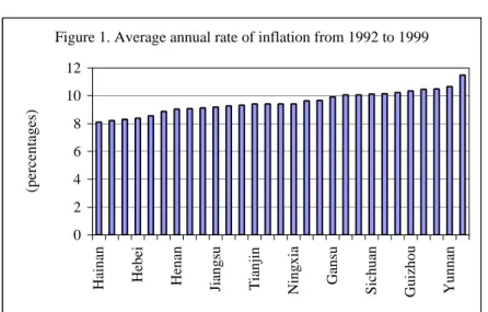
market economy was the difference between the rates of inflation of the provinces, not only for each year, but also in the long run. Thus, during recent years (from 1992 to 1999), the average annual rates of variation for the consumer price index in the Chinese provinces have ranged from 8.1 % for Hainan province to 11.5 % for Beijing municipality (figure 1), corresponding to a maximum gap in the rates of inflation of 40 % over ten years.
The diversity in the provincial rates of inflation in China is a priori surprising, as the twenty-nine Chinese provinces considered in this study constitute a monetary union1. If we apply the Mundell-Fleming model to a monetary union, the growth of the money supply in the different provinces would not differ on a long-term basis. Indeed, in an environment of free internal movement of goods and capital, a credit expansion which occurs more quickly in one province than in the rest of the monetary union causes a balance of payments deficit for this
1China is composed of 22 provinces (Hebei, Shanxi, Liaoning, Jilin, Heilongjiang, Jiangsu, Zhejiang, Anhui,
Fujian, Jiangxi, Shangdong, Henan, Hubei, Hunan, Guangdong, Guangxi, Hainan, Sichuan, Guizhou, Yunnan Shaanxi, Gansu and Qinghai), four autonomous municipalities under the direct control of the central government (Beijing, Tianjin, Shanghai and Chongqing), and five autonomous regions (Inner Mongolia, Guangxi, Tibet, Ningxia and Xinjiang). In our econometric analysis, the autonomous region of Tibet is absent due to a lack of statistics; the statistics for Chongqing, created in 1997, have been included with those for Sichuan, which means that 29 provinces, in the general sense of the word, have been retained.
Figure 1. Average annual rate of inflation from 1992 to 1999
0 2 4 6 8 10 12
Hainan Hebei Henan Jiangsu Tianjin Ningxia Gansu Sichuan
Guizhou Yunnan
province vis-à-vis the other provinces, and consequently a reduction in the money supply. That being the case, prices in the different provinces tend towards the same level.
However, price convergence does not really occur in every monetary union. Persistent differences in inflation between major American cities have been noted, as well as between the different states of the European Monetary Union (ECB, 1999). This divergence is explained by the Balassa-Samuelson effect, according to which the equality of general price levels expressed in the same currency unit, called purchasing power parity, does not hold between countries with differing levels of development (Balassa, 1964; Samuelson, 1964). The ground of this effect applied to a monetary union is that the prices of non-tradable goods in each country depend on the level of productivity in the sector of goods traded between member countries of the union. This explanation concurs with the working of a market economy. Indeed, it supposes that the competition between states in the union is sufficiently strong for the prices of traded goods to be identical. It implies the existence of a genuine labor market with mobility of labor between sectors (but not between countries) and workers’ remuneration based on their productivity, as well as mobility of capital between sectors and countries.
Does this explanation apply to the Chinese economy? An alternative explanation has been suggested, according to which the differences in inflation between the Chinese provinces could result from the decentralization of monetary power causing a strong dispersion of the growth rate of bank credits in a context of weak economic and financial integration (Boyreau-Debray, 2000 and 2001). Indeed, when China first began its transition towards a market economy, trade barriers existed between the Chinese provinces. There were even export or import bans between provinces. These barriers were only gradually diminished (World Bank, 1994), but still exist today. Similarly, for a long time, the foreign exchange markets and the inter-bank markets were specific to each province. They were only unified in 1994. On the
other hand, the inequality in the per capita product growth of the different provinces favors the explanation provided by the Balassa-Samuelson effect.
In the following article, we attempt to estimate the extent to which the Balassa-Samuelson effect explains the observed differences in inflation between the Chinese provinces during the nineties. This analysis is an indirect way of testing whether China has become a market economy. The first section provides a theoretical analysis of the Balassa-Samuelson effect applied to a monetary union such as that of China. A three-good model is proposed. The second section presents two econometric models that are estimated on cross sectional and panel data.
1. The theoretical analysis of the differences in inflation between the Chinese
provinces based on the Balassa-Samuelson effect
The Balassa-Samuelson effect was first presented in order to explain why the exchange rate between two countries (with different currencies) deviates from the purchasing power parity, even in the long run, if the levels of per capita income are different. If one applies the same analysis to states or provinces (referred to here as countries) belonging to a monetary union, the temptation is to directly explain the differences in inflation within the union by the differences in per capita product growth, as the exchange rate between the member countries of the union is, by definition, constant (ECB, 1999). But in this case, one only considers the trade relations within the union, distinguishing goods and services which are traded between member countries and those which are not (called non-tradables).
The shortcoming in this procedure is that it leaves out the trade relations of the countries of the union with the states outside the union. However, the barriers to trade within the union are normally smaller than those presented to states outside the union, leading to a distinction between internationally traded goods and goods traded only within the union.
Moreover, the foreign trade partners of each member country of the union can be different, as can the kind and quality of the exported and imported goods, such that the prices of the internationally tradables in each of the member countries of the union develop in a different manner.
These two hypotheses would seem to be realistic for China. Although the transition of the Chinese economy towards a market economy was accompanied by a liberalization movement with respect to foreign trade, this mainly concerned manufactured goods and, to a much smaller degree, industrial raw materials as well as foodstuffs. Furthermore, although Japan and the US are the major foreign trade partners of most of the provinces, as well as Hong Kong with respect to exports from China, their share in the trade of each province is noticeably different. So, the share of imports coming from the US ranges from 33 % for Yunnan to 4 % for Tibet in 1998, and those coming from Japan range from 63 % for Tibet and 9 % for Inner Mongolia (see appendix 1). In a country as vast as China, the geographic position of the provinces necessarily influences the direction and the nature of their trade. Thus the northern provinces engage in a greater degree of trade with the countries of the former Soviet Union than the other provinces (for example Xinjiang).
This is why, in order to apply the Balassa-Samuelson effect to the Chinese provinces, we need take into account the double nature of their external trade: international trade and trade with the other Chinese provinces. This leads us to present a three-good model and the way in which the price of each good category is defined.
Moreover, the Balassa-Samuelson effect is only a supply-side explanation of the real exchange rate. It relies on strong hypotheses of constant returns to scale and perfect international and internal mobility of capital. If we relax these hypotheses, which would seem necessary in the case of China, we are forced to complete the initial model by introducing demand shifts (Gregorio et alii. 1994 a and b).
1.1 A three-good model
The Balassa-Samuelson effect is based on the distinction between prices of internationally tradable goods (PT) and the prices of non-tradable goods (PNT). Here, we suppose that there exists another category of goods, called semi-tradables, often protected by the government, such as some mineral and agricultural goods. These goods are protected either to satisfy the domestic market or to guarantee the revenues of producers.
For province ‘i’ of China, the price of the non-tradable goods (PiNT) depends on purely provincial supply and demand, whereas the price of internationally tradables (PiT) is exogenously determined by its foreign partners. The price of semi-traded goods (PiST) depends on supply and demand in the whole of China because of the government protection policy. It is also exogenously determined for each province. These three categories of goods correspond approximately to craftsmen’s goods and services for non-tradable goods, to manufactured goods and export crops for internationally tradables and to consumer’s energy products and foodstuffs, strongly protected vis-à-vis the exterior, for semi-tradable goods within China.
By expressing the price indices in logarithms, we can formulate for province ‘i’ two equations defining its general price index and the average of these same indices for its foreign trade partners ‘ji’. The price index in province ‘i’ is defined as following
NT i ST i T i i P P P P =α +β +(1−α −β) (1)
where α, β and 1−α −β represent the percentage of tradables, semi-tradables and non tradables in the price index respectively. The average price index for the foreign trade partners ‘ji’ of province ‘i’ is defined as2
2 In order to obtain a simple and testable model, it is necessary to suppose by simplification that the weighting of
each category of goods in the general price index (industrial goods, food and services) for the Chinese provinces and for their foreign countries is approximately the same. Although this hypothesis is not always reasonable, it is an usual one in studies testing the Balassa Samuelson effect. It is however less opened to criticism if the consumer price index is used to calculate the real exchange rate as in our following econometric analysis (Chinn 1997b).
NT ji ST ji T ji ji P P P P =α +β +(1−α −β) (2)
Thus, the real effective or average exchange rate of province ‘i’, called ri, can be defined as the ratio of the general price index for this province to the average of the general price indices of its trade partners, expressed in the same currency. We can assert this definition in logarithmic form as following:
i ji i
i P P n
r = − + (3)
where ni denotes the nominal effective or average exchange rate of province ‘i’ vis-à-vis its main foreign trade partners (ji)3.
1.2The determination of prices in the three goods categories and of the real effective
exchange rate of each province
We examine the determination of the prices of the three categories of goods before formulating an equation for the real effective exchange rate.
1.2.1 The price of internationally tradable goods
According to Balassa-Samuelson, we first assume that the relative purchasing power parity prevails only for tradable goods (due to commodity arbitrage), so that the prices of internationally tradable goods in each province (piT) and its foreign trade partners (
T ji
P ), converted into the same currency unit using the exchange rates, develop in the same manner. From this, maintaining the logarithmic expression, it follows that
i T ji T i P n P = − (4)
3 The nominal effective exchange rate of each province is defined as a geometric average of the indices of the
exchange rates of the renminbi in terms of the currencies of its main foreign partners, weighted by the relative value of the trade with these last ones.
In the same way, the average prices of internationally tradable goods in China as a whole (pcT) are equal to its foreign trade partners (
T jc
P ), converted into the same currency unit using the exchange rates as following:
c T jc T c P n P = − (5)
with nc the nominal effective or average exchange rate of China as a whole vis-à-vis its main foreign trade partners, calculated using the exchange rates of the renminbi in terms of foreign currencies4.
1.2.2. The price of non-tradable goods
An other main hypothesis of the Balassa-Samuelson effect is that, “under the assumption that prices equal marginal costs, intercountry wage-differences in the sector of traded goods will correspond to productivity differentials, while the internal mobility of labor will tend to equalize the wages of comparable labor within each economy” (Balassa, 1964, p586).
To illustrate this proposition, we follow De Gregorio, Giovannini and Wolf (1994). From the production functions of the two sectors (tradable and non tradable goods), these authors derive an equation of the relative price of non tradable goods which depends on the total productivity of factors in each province (for demonstration see appendix 2).
So, always log-differentiating the expression for prices, in any country,
NT T T NT T NT P P θ θ γ γ − = − +constant (6)
4 Although the Chinese provinces have all the same money (the renminbi), the nominal effective exchange rates,
called for each province ni and for China as a whole nc, are different since the direction of trade of each province
with θT
and θNT
are respectively the total factor productivity in the sector of tradable goods and in the sector of non tradable ones, while γTand γNTrepresent the output-labor elasticity in each sector (or the factor shares).
Most work on the link between real exchange rates and sectoral productivity has employed labor productivity rather than the total factor productivity measure suggested by the theory (see by example Strauss, 1999). But De Gregorio, Giovannini and Krueger (1994) have shown that this substitution is not innocuous, “since labor shedding may introduce substantial differences between changes in labor productivity and changes in total factor productivity” (De Gregorio & Wolf, 1994). This biais may be particularly relevant in developing countries with rapid growth as China.
We apply the equation (6) to each Chinese province and to its foreign partners, so,
NT i T i i NT i T i NT i P P θ θ γ γ − = − +constant (7) NT ji T ji T ji NT ji T ji NT ji P P θ θ γ γ − = − +constant (8)
Knowing that the price of tradable goods is determined internationally (equation 4), and by subtracting (8) from (7), we obtain:
− − − = + − NT ji T ji T ji NT ji NT i T i T i NT i i NT ji NT i P n P θ θ γ γ θ θ γ γ +constant (9)
1.2.3. The price of semi-tradable goods or goods traded within China
We refer again to the Balassa-Samuelson effect to explain the prices of goods traded within China, i.e. non-tradable internationally. Now we consider China as a whole. If we assume, as before, that the average nominal wage is the same in the sectors of tradables and semi tradables, in China as well as in its foreign trade partners, and that the relative prices of
these two categories of goods in China and in its foreign trade partners are equal to the inverse of their total factor productivity (corrected by factor shares):
ST c T c ST c ST c T c ST c P P θ θ γ γ − = − +constant (10) ST c T jc ST jc ST jc T jc ST jc P P θ θ γ γ − = − +constant (11)
Knowing that the prices of tradable goods is determined internationally (equation 5), and by subtracting equation (11) from equation (10), we obtain:
− − − = + − ST jc T jc T jc ST jc ST c T c T c ST c c ST jc ST c P n P θ θ γ γ θ θ γ γ +constant (12)
Finally, we may replicate the same argument for the foreign trade partners of China as a whole vis-à-vis the foreign trade partners of each province5, thus
− − − = + − − ST ii T ji T ji ST ji ST jc T jc T jc ST jc i ST ji c ST jc n P n P θ θ γ γ θ θ γ γ (13)
1.2.4. The equation for the real effective exchange rate of each province
Let us recall that the real effective exchange rate of province i is defined as the ratio of the general price index for this province to the average of the general price indices of its trade partners, expressed in the same currency, as
i ji i
i P P n
r = − + (3)
By subtracting equation (1) from equation (2),
) )( 1 ( ) ( ) ( jiNT NT i ST ji ST i T ji T i ji i P P P P P P P P − =α − +β − + −α −β −
From equations (4), (9), (12) and (13), we derive the following equation of the real effective exchange rate of each province (see appendix 3 for the detail of the derivation).
− − − + − − − − − = ST ji T ji T ji ST ji ST c T c T c ST c NT ji T ji T ji NT ji NT i T i T i NT i i r θ θ γ γ θ θ γ γ β θ θ γ γ θ θ γ γ β α ) 1 ( +constant (14)
All variables being in logs, the real effective exchange rate of a province i appears to be first a function of the difference between the gap of the total factor productivity of tradables sector vis-à-vis the non tradables one in province i and the same gap in its main foreign trade partners. Second it is a function of the difference between the gap of the total factor productivity of tradables sector vis-à-vis the semi tradables one in China as a whole and the same gap in the main foreign trading partners of the province i.
In order to estimate directly this last equation, we might classify the industry as tradable goods, the agriculture as semi-tradables and services as non tradables. But on one hand, these “proxies” of each sector are highly debatable, and on the other hand we could not estimate the total factors productivity for the Chinese provinces and for their foreign partners due to the lack of reliable data, mainly on the stock of capital by sector6.
That is the reason why we use the last assumption of Balassa who supposes that the “international difference in productivity is smaller in the services than in the production of tradable goods” (Balassa, 1964). It results that the relative productivity of the tradable goods sector to the non tradables one in the various countries might be a positive function of per capita product (Kravis and alii, 1983, Dollar 1992). Although the semi tradables are not services, but mainly food goods, we shall widen the Balassa’s assumption to suppose that the international difference of productivity are smaller in agriculture than in the manufacturing sector. So, the relative total factor productivity of the sector of tradables vis-à-vis the semi
6 The stock of capital is often approximately estimated from investment in fixed assets. However, the data of this
last one divided by industry, agriculture and services sectors are not available for all foreign trade partners of the Chinese provinces. As in many studies, we might replace total factors productivity by labor productivity, despite the substitution problem between labor and capital explained in De Gregorio Giovannini and Wolf (1994). We have thus calculated the labor productivity by sector for the foreign trade partners of the Chinese provinces according to the World Development Indicators 2001 of World Bank. But we then observed that the data relative to value added and employment for agriculture, industry and service sectors are not available for all the foreign trade partners of the Chinese provinces. Moreover, the obtained results seem unreliable for several countries (for
tradables one, in China as for the provinces’ foreign trade partners, is assumed a positive function of their per capita product7.
If we suppose that this function is linear, it results a new equation of the real effective exchange rate of the Chinese provinces which is the following (see appendix 3 for the derivation). ) ( ) )( 1 ( i ji i c i y y y y r = −α − −β − +constant (15)
The real effective exchange rate of each province is thus a function of the ratios of its per capita product both to that of its foreign trade partners and to that of China as a whole. This last equation may be easily estimated.
1.3. Public expenditure, terms of trade, rate of bank credits and the real effective
exchange rate equation
Rogoff (1992) and De Gregorio et alii (1994) demonstrated that it is only in the case of perfect international and domestic capital mobility that the relative price of non tradable goods depends only on productivity across sectors. This assumption eliminates the role of demand side factors in the determination of relative prices. If we assume at the opposite that the capital is internationally as well as intersectorally immobile, the production of each sector is now subject to decreasing returns to scale.
That being the case, an exogenous increase in the demand for non-tradable goods, mainly due to an increase in public expenditure for which the content of non-tradable goods is higher than that of private consumption, needs an increase in their relative price to shift labor to this sector (De Gregorio et alii 1994a).
Thus, equation (15) relating to the real exchange rate should be completed as follows:
example, the productivity ratio between the industrial sector and agriculture one is less 0.05 for Denmark, and 0.10 for Canada, while it is more than 250 for Vietnam).
C g y y y y ri =(1−α)( i − ji)−β( i − c)+(1−α−β)γi i + (16)
Similarly, a variation in the terms of trade has an effect on the relative price of non-tradable goods. Indeed, a rise in the price of exported goods, which is an improvement in the terms of trade for given prices of imports, has two effects. First, a rise in the price of exported goods causes a rise in wages, which tends to increase the price of non-tradable goods. Second, by increasing global income, the improvement in the terms of trade increases the demand for non-tradable goods implying a further increase in their price in order to re-establish market equilibrium. The effect of a rise of the price of imported goods, corresponding conversely to a deterioration in the terms of trade, is unclear. Although the first effect via the increase in wages in the sector of importable goods is the same and thus implies the increase in the price of non-tradable goods, the fall in income causes, on the contrary, a reduction in the demand for and production of non-tradable goods, and thus a decline in their relative price8.
Since the beginning of its transition towards a market economy, China has experienced progressive and partial openness of the capital account. The most realistic hypothesis would seem to be that of imperfect mobility of capital9. It therefore seems desirable to introduce the two factors of demand defined above into the equation for the real effective exchange rate for the Chinese provinces. Indeed, the rate of public spending for the Chinese provinces experienced a different evolution during the nineties (Guillaumont Jeanneney and Hua, 2001b). Moreover, it is probable that the terms of trade did not evolve in the same way.
Thus, equation (15) relating to the real exchange rate should be completed as
7 According the data of World Development Indicators 2001 of World Bank, the differences of labor productivity
between in the United States and China are 63607, 35188 and 23395 US dollars per employee in 1997 (constant 1995 US$), respectively for industry, agriculture and services sectors.
8
The Balassa-Samuelson model, completed by public spending and terms of trade, concurs with the analysis of the determinants of the long-term equilibrium real exchange rate for developing countries (Edwards, 1989; Hinkle and Montiel, 1999). The three “fundamentals” (per capita product, the rate of public spending and the terms of trade) are completed by variables representing foreign trade policy and international debt. These last two factors are eliminated here as they intervene for the whole of China.
9 In the hypothesis of total immobility of capital, De Gregorio (1994b) showed that the expected effect of
productivity growth in tradable goods activities becomes unclear. However, this hypothesis is extreme, as recognized by the author.
follows10: C T g y y y y ri =(1−α)( i − ji)−β( i − c)+(1−α −β)γi i +(1−α −β)δi i + (17)
with g= the ratio of public spending to GDP T= terms of trade
Finally, we completed the theoretical model by introducing a variable representing credit policy, specific to each province, in order to test the alternative explanation of dispersion of the inflation rates by province, linked to the fragmentation of the Chinese economy (Boyreau Debray, 2000).
C c T g y y y y ri =(1−α)( i − ji)−β( i − c)+(1−α−β)γi i +(1−α−β)δi i +(1−α−β)λi i+ (18)
with ci = rate of bank credits to the GDP of province i.
The equations from 15 to 18 are successively estimated econometrically in terms of two models, one based on cross sectional data, and the other based on panel data. The estimation on yearly panel data enabled us to increase the number of our observations and to estimate theoretical model, i.e. equations 15, 16, 17 and 18 directly.
The first complete estimated model is thus:
i i i i i i c i ji i i d y y d y y dg dT dc dr =(1−α) ( − )−β ( − )+(1−α−β)γ +(1−α−β)δ +(1−α−β)λ
which can also be expressed as:
c i i i i i i ji i i dy dy dg dT dc dy dr =(1−α−β) −(1−α) +(1−α−β)γ +(1−α−β)δ +(1−α−β)λ +β
This model implicitly supposes that the real exchange rates and the per capita products follow a determinist trend.
The final term of the equation (βdyc), which depends on the rate of growth of China, corresponds to the constant of the equation. It is possible that this constant also reflects the factors, common to China as a whole, which could have influenced its real effective exchange
10
A complete model should take into account the variables relative to public expenditure and terms of trade for foreign trade partners for each province and for China as a whole in the hypothesis of non-perfect capital
rate, such as a liberalization of foreign trade policy acting in the direction of a depreciation of this rate.
The second complete model, estimated in panel and the variables again expressed in logarithmic form, is as follows:
c c T g y y y y ri =(1−α)( i− ji)−β( i− c)+(1−α−β)γi i +(1−α−β)δi i+(1+α+β)λi i+ +fixed effects
Here, the difference between the logs of per capita products of province i and of its foreign trade partners on the one hand, and between that of province i and China on the other hand, become explanatory variables. Fixed effects are necessary, as the estimated variable is an index, the identical base of which for all the provinces cannot take into account the relative initial price level in the different provinces. We present the calculation of the variables before the results of the two models.
2. Econometric estimation of the real effective exchange rates of the Chinese
provinces
As we have seen, determining the real effective exchange rate of the Chinese provinces, according to the Balassa-Samuelson analysis, supposes that the Chinese economy broadly works like a market economy. That is why we have limited our estimation for a recent period, i.e. 1992-1999. Indeed, since 1992, the economic liberalization has sharply increased after several years of reform inertia in order to fight against economic overheating. The first model based on cross sectional data is thus estimated using the average rates of growth for the period 1992-1999, except for the rate of growth of the foreign trade partners of each province which is calculated for the period 1992-1998. The second model is based on yearly panel data for the 1992-1998 period. 11
mobility in these countries. We have dropped them for simplification.
11 As an anonymous referee suggested to us, it is interesting to repeat the estimation for a period prior to 1992,
which would strengthen the argument if the results appear to be different. But one innovation of our model is to take in account the diversity of foreign trade partners of the Chinese provinces. Unhappily the data for the
2.1. Presentation of the variables
2.1.1. The dependent variable: the real effective exchange rate of each province
Since the beginning of the Chinese transition towards a market economy, its exchange rate policy has experienced two phases (Guillaumont Jeanneney and Hua, 2001a). Until 1994, that is during the first two years of our period of estimation, China maintained two exchange rates of the dollar vis-à-vis the yuan for trade operations; an official rate and a higher “swap” rate, determined on the foreign exchange markets but in fact strictly controlled by the central authorities. Export companies were to sell 20 % of the foreign currency earned at the official rate and could either use the remaining 80 % for their own imports or sell them on the foreign exchange markets at the swap rate. The imports considered by the government as having priority were financed at the official rate and the other imports at the swap rate. The latter depreciated dramatically in 1992, while the official rate was devalued before the unification of the two exchange rates at the beginning of 1994. Having experienced a depreciation in the first year, the unique exchange rate has slightly appreciated since then.
Thus, for the period 1992-93, an exchange rate of the dollar vis-à-vis the yuan was calculated as a weighted average of the official and swap rates, the weighting resulting from the sum of the transactions on the exchange markets compared to imports. The real effective exchange rate indices of the Chinese provinces were calculated, with a base of 1990 = 100, as the ratio of the consumer price index of each province to the weighted geometric average of the consumer price indices, converted into yuans, the weighting resulting from the import
direction of trade of the provinces are only available since 1995. (They are not published, but can be obtained from China’s Customs General Administration.) As the structure of foreign partners is very different for China as a whole in 1980s and in 1990s, it is likely to be the same for each province. Korea Republic, Taiwan province and Vietnam did not trade with China for example before 1990. However we still did a tentative estimation for the period 1984-1991, using the same structure of foreign trade partners as for the period 1992-1999, after having removed out Korea, Taiwan and Vietnam.
structure of the first fifteen trade partners for imports by province 12 in 199813. The above choice of import-side for weightings is justified by the fact that the prices of imported goods seem to influence the consumer price level more than the prices of exported goods.
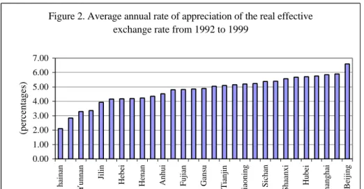
The nominal weighted exchange rate of yuan against dollars is not the same in 1992 and 1993 for all the provinces because the swap rate is different for each province (Khor, 1993). Even though the Chinese provinces have the same nominal exchange rate against dollar for the rest of the estimation period, their real effective exchange rate has evolved differently due to the disparities in their inflation rates and the diversity of their foreign trade partners. Over the whole of the estimation period 1992-1999, the average annual appreciation of the real effective exchange rates of the Chinese provinces ranges from 2.1 % for the province of Hainan to 6.6 % for the municipality of Beijing (cf. figure 2).
12
Unfortunately, we were obliged to eliminate some countries of the former Soviet Union, for which data pertaining to the exchange rate were not available. The exchange rate and consumer price indices are taken from the IMF, International Financial Statistics for the foreign trade partners of the Chinese provinces. The import structure data of each province are from China’s Customs general Administration. The consumer prices indices of each province are from China Statistical Yearbook. The swap rates of the Chinese provinces in 1992 and 1993 are originated from Khor (1993).
13 Year for which we were able to procure the origin of imports in the different provinces from China’s Customs
General Administration.
Figure 2. Average annual rate of appreciation of the real effective exchange rate from 1992 to 1999
0.00 1.00 2.00 3.00 4.00 5.00 6.00 7.00
hainan Yunnan Jilin Hebei Henan Anhui Fujian Gansu Tianjin
Liaoning Sichan Shaanxi
Hubei
Shanghai Beijing
2.1.2. The independent variables
The per capita GDP of China (yc)and of each province (yi) was calculated as the ratio of GDP, expressed in yuans (constant 1995 value) and converted into dollars by the 1995 exchange rate of the yuans vis-à-vis the dollar (i.e. according to the method of the World Bank), to the population. The data are drawn from the Comprehensive Statistical Data and Materials on 50 years of New China, and China Statistical Yearbook 2000. We also used the GDP divided by the population in employment, which did not alter the results. The per capita GDP of the foreign partner countries of each province (yji) corresponds to the weighted geometric average of their GDP also expressed in dollars at the constant 1995 value and divided by the population. The weighting is identical to that used to calculate the real effective exchange rates. The GDPs are taken from the World Bank World Development Indicators, and the populations from the IMF, International Financial Statistics.
The rate of budget expenditure of each province (gi) is the ratio of budgetary spending (taken from China’s Statistical Yearbook) to the GDP. We chose here to use the rate of budgetary spending in its strictest sense, eliminating extra-budgetary expenditure, because only the former corresponds exclusively to consumer spending (Guillaumont Jeanneney and Hua 2001b) for which we can consider that the content in non-tradable goods is higher than that of private spending. We would have preferred to use a rate of public spending in volume, but unfortunately this was not available to us14. The average rate of budgetary spending of the provinces from 1992 to 1999 varies between 5.5 % for Jiangsu and 20.2 % for Yunnan (cf. figure 3).
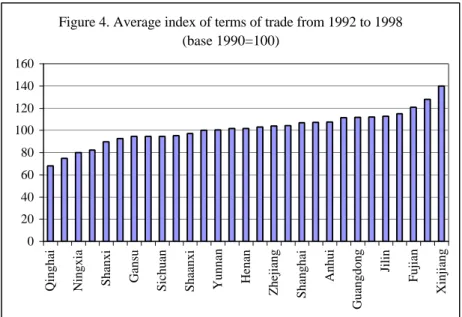
The terms of trade were not officially published for China as a whole, not a fortiori for each province for the 1992-1999 period. They have been calculated using the data of China’s Customs General Administration with the base 100 in 199015. The terms of trade for each province, defined as the ratio of export unit value index relative to import unit value index, varies significantly because their foreign trade partners and the nature of their exported and imported goods are very different. The average index of terms of trade of the provinces for the 1992-1998 period varies between 68 for Qinghai and 140 for Xinjiang (cf. figure 4).
15 We thank Yue Changjun for the calculation of the terms of trade. The data used to calculate the provincial
terms of trade (TOT) are from China’s Customs General Administration, according to 4-digit Standard International Trade Classification (SITC), given by province of export (import), countries of purchase (sale), unit of quantity, value, and quantity. These data, only available in 1990s, are not published, but can be obtained from China’s Customs General Administration. This is another reason why we have limited our estimation in 1990s. Export or import unit value is firstly calculated for each product as the ratio of its export or import value to its quantity for each year from 1991 to 1998. Those products, which are not exported or imported in the former year, are dropped, as well as those whose price indices are either higher than 150% or lower than 50% relative to the preceding year. Second, the export or import unit value index is computed for each province as the weighted geometric average of the export or import unit value index for each product. The ratio of export or import value of each product relative to the total export or import value of each province is used for the weighting. The TOT is obtained by dividing the export unit value index by the import unit value index, taking first the preceding year as the base 100, and then 1990 as the unique base year.
Figure 3. Average ratio of budgetary expenditure to GDP from 1992 to 1999 0 5 10 15 20 25
Jiangsu Hebei Anhui Hunan Jiangxi Guangxi Shaanxi Hainan Gansu Qinghai
Finally, credit policy was represented by the rate of growth of bank credits to the economy in each province in the cross-sectional model and by the ratio of these credits to the GDP of each province in the panel model (the data relating to bank credit are taken from
China Regional Economy, A Profile of 17 Years of Reform and Opening-Up and Comprehensive Statistical Data and Materials on 50 years of New China). Figure 5 shows that each province presents a different ratio of bank credits to GDP for the 1992-1998 period, varying from 45 % for Zhejiang to 129 % for Qinghai.
Figure 4. Average index of terms of trade from 1992 to 1998 (base 1990=100) 0 20 40 60 80 100 120 140 160
Qinghai Ningxia Shanxi Gansu Sichuan Shaanxi Yunnan Henan Zhejiang
Shanghai Anhui Guangdong Jilin Fujian Xinjiang
2.2. The results of the econometric estimation16.
2.2.1 Preliminary tests: stationarity and exogeneity
In recent years, numerous authors have attempted to apply the Balassa-Samuelson effect to the OECD countries, basing their work on an analysis of co-integration of the price and productivity variables (Asea and Mendoza 1994, Canzoneri et alii 1996, Chinn 1997a). Strauss (1999), however, showed that, contrary to the most commonly accepted opinion, using a panel stationarity test allowed that the null of stationarity for the same OECD countries cannot be rejected. The Im-Pesaran-Shin test is used here to examine the null of stationarity of real effective exchange rate, the two differences of products, ratio of budgetary expenditure, terms of trade and ratio of bank credits. The panel t-statistics, reported in table 2, allow us to significantly reject at the 1% level the null hypothesis of a unit root for these variables.
Given the role played by the evolution of the real effective exchange rate in the growth of Chinese exports (Guillaumont Jeanneney and Hua, 1996), and thus in the rhythm of
16 STATA 6.0 and Eview 3.1 are used in econometric estimation.
Figure 5. Average ratio of bank credits to GDP for 1992-1998 period 0 20 40 60 80 100 120 140 Zhejiang Fujian Henan Shangdong Jiangxi Guizhou Inner Mongolia Shanghai Ningxia Jilin (percentages)
economic growth, the endogeneity of the growth variable of the Chinese provinces is likely. The risk of endogeneity is greater for panel estimation using annual data than for cross sectional analysis. Indeed, the causality relation running from the real exchange rate towards growth is a short-term phenomenon, whereas the inverse relation, which corresponds to the Balassa-Samuelson effect, is a long-term relation. So in the first model, we test the exogeneity of the average per capita product growth rate of the Chinese provinces and in the second model, that of the differences between the per capita income in each province and either the average per capita income for China or the average per capita income of its foreign trade partners, all variables being then expressed in logs.
In the first model on cross sectional data, the instrumental variables of the per capita product growth rate of the Chinese provinces are the population density (popd92 ) and thei real per capita product (y92 ) in 1992 as well as the education variables. These last variables,i calculated as an average for the 1992-1998 period, measure the human capital of each province and correspond to the proportions of the population having received up to primary, secondary and university education respectively (edupi,edusi,and eduui) (Démurger, 1998). The impact of the initial product can be positive if it represents the endowment in capital, notably in infrastructure, or negative if there is a convergence effect. With respect to the second model on panel data, the instrumental variables retained for the difference in income between each province and its foreign partners are the per capita product of the foreign trade partners (yji), the three education variables and the rate of industrial production compared to global production (prodi) (China Statistical Yearbook). Indeed, this last variable, structural in nature, is representative of the growth potential of each province and is not correlated to the real exchange rate. However, population density noted annually is influenced by the competitiveness of the economy.
growth rate in the Chinese provinces proved to be exogenous by the application of the Davidson-MacKinnon exogeneity test, completed by Sargan’s over-identification test. On the other hand, in the second model on panel data the differences in per capita product appeared to be endogenous in the second model and we thus proceeded to carry out estimation by TSLS.
2.2.2 The results on cross sectional and panel data
The results of the two models of the real effective exchange rate of the Chinese provinces are shown respectively in tables 1 and 2.
With respect to the first model, the per capita product growth rate of each province and the rate of budgetary spending have the expected signs with a significance of 5 % and 1 % respectively. The appreciation of the real exchange rate of each province appears to be a positive function of its per capita income growth and of the growth rate of its budgetary expenditure ratio. Nonetheless, the growth rate of foreign trade partners has the expected negative sign, but with a very weak significance (22%). This disappointing result could be due to the fact that it was impossible to include certain countries from the former Soviet Union, although these countries are important trade partners of certain provinces. The rate of variation of the rate of budgetary expenditures is also very significant while this is not the case for the variation of terms of trade. We know that for this last variable the expected sign is ambiguous.
Let us also note that the constant in the equation, equal to (βdyc) according to the theoretical model, corresponds to a per capita average growth rate for China over the period 1992 to 1999 of 7.15 % (regression 3) for an observed growth of 9.6 %.
Introducing the bank credit growth rate, whose coefficient is not significantly different from zero, enables us to refute the explanation of a durable difference in inflation between the provinces by the disparity in bank credits (regression 4).
The final column of table 1 presents, in parallel, the results of an estimation of the inflation rate for each province as a function of its per capita product growth rate. The poor result of this estimation shows that the influence exercised by the growth rate on prices cannot be brought to light without taking into account the impact of trade between the provinces and the outside, a fact which permits the estimation of the real effective exchange rate17.
Table 2 presents the results of the estimation based on panel data now distinguishing the estimations in OLS and TSLS. The two estimations of the basic model (regressions 8 and 12) differ little. All the variables, even the terms of trade are significant at the 1% level, with the exception of the coefficient for the difference in income between each province and China, which is only significant at 10 % in TSLS. The real exchange rate of each province (on an annual base) is well a positive function of the gap of its real per capita income to the average per capita income of its foreign partners, of its budgetary expenditure ratio and of its terms of trade. It is a negative function of the gap of its per capita income to that of China as a whole. If we compare regression (12) in table 2 to regression (3) in table 1, it appears that the coefficients αand β are rather similar, i.e. αequals respectively 0.20 and 0.12 whileβequals 0.64 and 0.74. Thus, there is very little difference between the results of the Balassa-Samuelson effect estimations whether they are cross sectional or panel.
However, when we introduce the rate of bank credits into the panel estimation (regression 13), the latter is statistically significant at the 1% level, whereas the difference in the product of each province compared to that of China no longer is. This result suggests that
17 This conclusion is strengthened by the fact that if the real exchange rate of each province is only regressed on
its per capita product growth, this last variable is no longer significant. In fact, if we suppose that the foreign trade partners are the same for each province, the equation 15 becomes the simple relation between real exchange rate of each province and its per capita product. That is the reason why, due to the lack of data on the direction of trade of the Chines provinces in the1980s, replicating the estimation of the real exchange rate for a previous period is a little hazardous (cf. note 11). However we may note that the same regression for the previous period 1984-1991 does not give significant results for the rate of growth of the provinces, as well as for that of their foreign trade partners. This justifies the choice of a recent period for testing the Balassa-Samuelson effect (Results not reported in the table).
monetary policy, which is not uniform throughout China, exercises a short-term influence both on the level of production and on the price level (Brandt and Zhu, 2000), and that, effectively, mobility of capital and merchandises between the provinces is not perfect at least in the short term.
Conclusion
Although the econometric analysis was limited by the availability of data, it does not refute the hypothesis that the Balassa-Samuelson model explains the durable differences in inflation between the Chinese provinces. It suggests that the Chinese economy broadly works as a market economy, even if there remain some obstacles to the exchange of goods and capital between provinces. With respect to economic policy, it implies that an identical inflation objective for all the Chinese provinces would not necessarily be relevant.
Appendix 1. The 20 main import partners for each Chinese province in 1998
Beijing Tianjin Hebei Shanxi Inner Mongolia Liaoning Jilin Heilongjian
g
Shanghai Jiangsu
US 21.54 Japan 26.57 Japan 18.08 US 27.65 Russia 22.47 Japan 29.75 Germany 36.66 US 16.35 Japan 25.52 Japan 21.02
Japan 13.05 Korea Rep 18.67 US 13.04 Australia 14.12 US 17.26 Korea Rep 14.26 US 11.61 Russia 14.15 US 16.44 Taiwan prov 10.15 Germany 7.92 US 16.89 Korea Rep 9.38 France 9.56 Mongolia 12.81 Russia 14.03 Japan 10.36 Korea Rep 11.84 Germany 9.61 Korea Rep 9.04 Korea Rep 7.66 Taiwan prov 5.61 Russia 6.55 Japan 9.39 Germany 10.78 US 11.17 Italy 5.83 Sweden 11.82 Korea Rep 6.88 US 7.84 Canada 5.53 Hong Kong 5.54 Canada 6.45 Germany 6.11 Japan 8.55 Germany 2.43 Korea Rep 5.77 Japan 11.46 Taiwan prov 6.87 Germany 6.80 Sweden 4.76 Singapore 3.50 Germany 5.80 UK 5.94 Australia 7.44 Australia 2.34 Brazil 4.08 Germany 10.54 Hong Kong 5.50 Singapore 5.60 Russia 4.48 Germany 3.28 Sweden 5.77 India 4.56 UK 3.31 Saudi Arabia 2.30 Russia 2.89 France 3.62 Singapore 2.87 Thailand 3.27 Finland 4.17 Malaysia 2.63 Australia 4.18 Canada 3.81 Korea Rep 2.39 Taiwan prov 1.95 Sweden 2.87 Italy 3.15 France 2.72 France 2.98 Singapore 2.82 Russia 1.67 Philippines 2.66 Russia 3.53 Thailand 2.12 Indonesia 1.81 Australia 2.36 Argentina 1.87 Australia 2.60 Sweden 2.89 Hong Kong 2.71 Indonesia 1.65 France 2.48 Korea Rep 2.50 Malaysia 1.74 Sweden 1.67 Canada 2.29 Spain 1.48 Malaysia 1.80 Finland 2.83
UK 2.14 UK 1.60 Argentina 2.42 Taiwan prov 1.47 Italy 1.72 UK 1.49 Mexico 2.29 India 1.38 Indonesia 1.76 Hong Kong 2.67
France 2.07 France 1.12 Italy 2.11 Vietnam 1.42 Singapore 1.20 Canada 1.07 France 1.96 Brazil 1.32 Brazil 1.75 Indonesia 2.49 Australia 1.90 Italy 1.06 Taiwan prov 2.06 S.Africa 1.31 France 0.93 Singapore 1.07 Korea 1.94 Canada 1.31 Italy 1.72 Italy 2.46 Italy 1.69 Argentina 1.01 Tunisia 2.03 Italy 1.15 Netherlands 0.93 Italy 1.05 India 1.39 UK 1.14 Canada 1.29 Malaysia 1.81 Brazil 1.49 Brazil 0.96 UK 1.76 Malaysia 0.92 Taiwan prov 0.90 Mongolia 0.85 Malaysia 1.09 Taiwan prov 1.00 Belgium 1.28 Australia 1.67 Malaysia 1.36 Canada 0.95 Brazil 1.65 Ecuador 0.84 India 0.88 China 0.79 Taiwan prov 1.01 Malaysia 0.95 UK 1.27 Canada 1.51 Peru 1.32 Australia 0.83 India 1.62 Thailand 0.74 Israel 0.81 India 0.76 UK 0.95 Singapore 0.78 Netherlands 1.16 Russia 1.25 Taiwan prov 1.06 Philippines 0.58 Malaysia 1.44 Switzerland 0.74 Finland 0.77 France 0.73 Netherlands 0.59 Indonesia 0.62 Thailand 0.89 UK 1.20 Argentina 1.02 Thailand 0.55 Spain 1.29 N. Zealand 0.67 Sweden 0.62 Iraq 0.71 Gabon 0.40 Belgium 0.53 Sweden 0.69 Netherlands 1.05 Indonesia 0.87 Spain 0.43 Ecuador 1.29 Netherlands 0.54 Indonesia 0.53 Argentina 0.61 S.Africa 0.35 Austria 0.51 Switzerland 0.68 Brazil 1.04
Zhejiang Anhui Fujian Jiangxi Shandong Henan Hubei Hunan Guangdong Guangxi
Japan 20.77 Germany 14.66 Taiwan prov 28.79 Japan 14.84 Korea Rep US 18.03 US 19.96 Germany 11.28 Japan 21.11 France 17.52
US 12.46 Chlie 12.68 Japan 16.20 US 9.81 Japan 29.66 Australia 11.85 France 17.05 US 9.906 Taiwan prov 19.56 US 9.23
Korea Rep 11.35 Japan 10.03 Korea Rep 12.26 Canada 8.13 US 14.17 Japan 10.76 Japan 14.26 Korea Rep 9.521 Korea Rep 9.96 Japan 7.82
Taiwan prov 6.55 US 8.25 US 8.94 UK 7.66 Russia 13.32 France 6.551 Australia 6.528 Japan 9.301 US 8.41 Russia 5.31
Germany 4.09 Australia 8.25 Germany 4.30 Germany 6.97 Germany 4.79 Russia 5.878 Germany 5.867 UK 4.912 Hong Kong 7.58 Sweden 5.27 Canada 3.81 Korea Rep 7.50 Hong Kong 3.30 Korea Rep 6.23 Taiwan prov 4.77 Korea Rep 5.536 Sweden 4.362 Israel 4.681 China 4.88 Korea Rep 4.35 Iran 3.57 Oman 4.32 Indonesia 2.80 Russia 6.02 Australia 2.68 Germany 4.684 Korea Rep 3.466 Australia 4.401 Singapore 3.81 Taiwan prov 4.24 Italy 3.56 Brazil 3.37 Singapore 2.38 Taiwan prov 5.04 Hong Kong 2.67 Italy 4.603 Indonesia 2.863 France 4.114 Thailand 2.57 UK 4.03 UK 3.07 Italy 2.97 Malaysia 2.32 Indonesia 4.65 Italy 2.34 India 3.502 S.Africa 2.13 Austria 3.796 Malaysia 2.41 S.Africa 3.67 Indonesia 2.76 Taiwan prov 2.95 China 2.15 Hong Kong 3.92 Canada 2.00 Canada 2.851 Italy 2.06 Taiwan prov 3.535 Germany 2.27 India 3.56 Australia 2.51 Canada 2.06 UK 1.94 Australia 2.88 Sweden 1.89 UK 2.592 Canada 1.984 India 3.362 Indonesia 1.82 Germany 3.55 France 2.18 Mongolia 2.00 Thailand 1.76 Oman 2.88 India 1.47 Taiwan prov 2.305 Taiwan prov 1.63 Switzerland 3.293 Russia 1.15 Vietnam 3.22 Hong Kong 2.10 Russia 1.86 Italy 1.48 Italy 2.44 Spain 1.43 Netherlands 2.303 Hong Kong 1.532 Canada 3.24 Australia 1.14 Canada 3.08 Oman 2.04 India 1.51 Russia 1.34 Morocco 1.88 Argentina 1.40 Hong Kong 1.899 Russia 1.452 Oman 2.717 UK 0.93 Australia 2.76 Argentina 1.96 Malaysia 1.46 Oman 0.99 Chlie 1.77 Oman 1.26 Singapore 1.788 UK 1.431 Indonesia 2.653 France 0.91 Italy 2.16 Malaysia 1.56 Indonesia 1.43 Australia 0.88 France 1.71 Brazil 1.16 Indonesia 1.715 Oman 1.406 Italy 2.58 Italy 0.85 Finland 2.06
Russia 1.31 UK 1.30 France 0.80 Spain 1.56 Thailand 1.16 Thailand 1.695 Gabon 1.305 Russia 1.976 S.Africa 0.79 Malaysia 2.03 Singapore 1.18 Singapore 1.28 Finland 0.78 Mongolia 1.44 Malaysia 1.10 Malaysia 1.481 Malaysia 1.254 Peru 1.974 Saudi Arabia 0.74 Switzerland 1.66 Thailand 0.99 France 1.19 Canada 0.68 S.Africa 1.36 Indonesia 1.08 S.Africa 0.807 Brazil 0.847 Netherlands 1.475 Sweden 0.73 Gabon 1.64 Republic of
Yemen
0.97 Hong Kong 0.91 Saudi Arabia 0.51 Singapore 1.27 UK 1.01 Uzbekstan 0.736 Netherlands 0.834 S.Africa 1.299 Canada 0.70 Hong Kong 1.63
Hainan Sichuan Guizhou Yunnan Tibet Shaanxi Gansu Qinghai Ningxia Xinjiang
US 33.61 Japan 26.72 US 32.82 US 32.82 Japan 63.14 France 37.36 US 23.85 US 52.65 US 34.33 Kazakhstan 33.67
Russia 14.43 US 19.10 Japan 10.44 Italy 9.08 Nepal 8.56 Japan 13.28 Australia 16.48 Japan 20.11 Japan 11.50 US 24.38
Japan 14.39 France 12.01 Italy 8.72 Germany 8.16 Korea Rep 5.32 US 13.17 Japan 11.02 Korea Rep 7.16 Canada 10.26 France 10.07 Korea Rep 5.55 Germany 9.27 India 6.35 Myanmar 5.77 US 4.00 Belgium 5.42 Germany 9.51 Jamaica 5.17 Australia 8.40 Japan 7.32 Singapore 4.38 Italy 3.77 Australia 6.28 Chlie 4.19 Russia 3.24 Germany 3.88 Mongolia 6.88 Germany 3.80 Korea Rep 7.83 Russia 4.73 Italy 4.00 Canada 3.25 Germany 4.24 Canada 3.96 Germany 2.68 Sweden 3.64 Korea Rep 6.18 Russia 1.83 Thailand 4.70 Germany 3.52 Taiwan prov 3.12 Australia 3.07 Korea Rep 3.71 Japan 3.29 Malaysia 2.50 Italy 3.16 Italy 4.61 Italy 1.76 Malaysia 3.98 Kirghizia 2.45 Germany 2.81 Switzerland 2.78 Thailand 2.93 Australia 3.02 Indonesia 1.99 Korea Rep 3.15 Russia 4.06 Malaysia 1.48 Finland 3.23 Canada 2.34 Hong Kong 2.44 Taiwan prov 2.69 Malaysia 2.46 UK 2.35 N. Zealand 1.69 UK 2.66 Argentina 3.56 Canada 1.32 Sweden 2.91 Korea Rep 1.60 Thailand 1.99 Russia 2.57 Singapore 2.13 India 2.27 Australia 1.65 Australia 2.31 Peru 3.48 Indonesia 1.22 UK 2.15 UK 1.45 Malaysia 1.71 Korea Rep 2.36 Finland 1.96 Switzerland 2.20 France 1.01 Russia 1.81 Taiwan prov 1.66 Denmark 0.89 Rwanda 1.17 Israel 0.70 Vietnam 1.35 UK 1.95 Switzerland 1.85 Taiwan prov 2.15 Ukraine 0.98 Taiwan prov 1.44 France 1.48 N. Zealand 0.76 Indonesia 1.15 Australia 0.65 Netherlands 1.17 Malaysia 1.49 Taiwan prov 1.81 Russia 2.06 Singapore 0.86 Ireland 1.35 UK 1.41 Taiwan prov 0.36 France 1.11 Tadzhikistan 0.59 Ukraine 0.95 Sweden 1.25 Indonesia 1.80 S.Africa 1.84 Thailand 0.55 Spain 1.15 Cuba 1.03 France 0.34 Italy 1.01 Singapore 0.56 Belgium 0.77 Hong Kong 1.16 Hong Kong 1.76 Hong Kong 1.63 Switzerland 0.50 Kazakhstan 0.79 Canada 0.90 Hong Kong 0.34 Hong Kong 0.83 Italy 0.53 Canada 0.70 Netherlands 0.75 Canada 1.54 France 1.60 Hong Kong 0.35 Netherlands 0.74 Finland 0.79 Australia 0.21 Netherlands 0.83 Finland 0.48 Switzerland 0.69 India 0.72 Gabon 1.49 Austria 1.53 Taiwan prov 0.30 Hong Kong 0.64 Ghana 0.55 Sweden 0.20 Russia 0.82 Austria 0.39 Norway 0.65 Singapore 0.63 UK 1.24 Korea Rep 1.52 Kazakhstan 0.26 Switzerland 0.45 Netherlands 0.30 Mexico 0.17 Germany 0.72 Belgium 0.35
UK 0.62 Kazakhstan 0.42 France 1.15 Vietnam 1.04 Belgium 0.22 Canada 0.41 Belgium 0.29 UK 0.17 Norway 0.45 Spain 0.35
Australia 0.58 Indonesia 0.41 Russia 1.12 Singapore 1.04 Canada 0.17 Fiji 0.34 Malaysia 0.22 Singapore 0.05 Mongolia 0.39 Sweden 0.34
Appendix 2. The derivation of the relative price equation of non tradable goods
We follow the demonstration of De Gregorio, Giovannini and Wolf (1994) to derive the relative price equation of non tradable goods. These authurs begin with the production function of each sector, i.e.
) 1 ( T T T T T T K L Q =θ γ −γ (1a) ) 1 ( NT NT NT NT NT NT K L Q =θ γ −γ (2a)
where T and NT denote tradable and non tradable goods, Q denotes output, L labor input and K capital. Under perfect competition, price in each sector are derived by duality as: ) 1 ( ) 1 ( ) 1 ( 1 T T T T T T T T R W P γ γ γ γ γ θ γ − − − − = − (3a) ) 1 ( ) 1 ( ) 1 ( 1 NT NT NT NT NT NT NT NT R W P γ γ γ γ γ θ γ − − − − = − (4a)
where W is the unit cost of labor and R the rate of return on capital.
Supposing that the rate of return on capital is equal to its world value (due to the law of one price in tradable goods sector and perfect capital mobility), and log differentiating the expression for prices and solving for difference, it results that
W P
PNT − T =θT −θNT +(γNT −γT) +constant (5a)
Taking PTas numeraire and assuming that R is constant, log-differentiating equation (3a) and substituting into the equation (5a) yields an expression for the relative price of nontradable goods: NT T T NT T NT P P θ θ γ γ − = − +constant
Appendix 3. The derivation of the real exchange rate equation
Recall the equations (1), (2) and (3) in the article as following NT i ST i T i i P P P P =α +β +(1−α −β) (1) NT ji ST ji T ji ji P P P P =α +β +(1−α −β) (2) i ji i i P P n r = − + (3)
with P consumer price index expressed in logarithms.
By subtracting equation (1) from equation (2), we obtain
) )( 1 ( ) ( ) ( iT jiT iST jiST iNT jiNT ji i P P P P P P P P − =α − +β − + −α−β −
Recall the equations (4) and (9) such as,
i T ji T i P n P − =− (4) i NT ji T ji T ji NT ji NT i T i T i NT i NT ji NT i P n P − − − − = − θ θ γ γ θ θ γ γ +constant (9)
We obtain the following equation of real effective exchange rate,
− − − − − − + − + − = − i NT ji T ji T ji NT ji NT i T i T i NT i ST ji ST i i ji i P n P P n P θ θ γ γ θ θ γ γ β α β α ( ) (1 ) +constant − − − − − + − + = + − NT ji T ji T ji NT ji NT i T i T i NT i ST ji ST i i i ji i P n n P P P θ θ γ γ θ θ γ γ β α β( ) (1 ) +constant (17) Recall equation (13), − − − = + − − ST ii T ji T ji ST ji ST jc T jc T jc ST jc i ST ji c ST jc n P n P θ θ γ γ θ θ γ γ +constant (13)
the first term of the equation (17) is expressed as following :
− − − + + − = + − ST ji T ji T ji ST ji ST jc T jc T jc ST jc c ST jc ST i i ST ji ST i P n P P n P θ θ γ γ θ θ γ γ +constant
Recall the equation (12) as, − − − = + − ST jc T jc T jc ST jc ST c T c T c ST c c ST jc ST c P n P θ θ γ γ θ θ γ γ +constant (12) and as cST ST i P
P = , we obtain the following equation as,
− − − + − − − = + − ST ji T ji T ji ST ji ST jc T jc T jc ST jc ST jc T jc T jc ST jc ST c T c T c ST c i ST ji ST i P n P θ θ γ γ θ θ γ γ θ θ γ γ θ θ γ γ +constant − − − = + − ST ji T ji T ji ST ji ST c T c T c ST c i ST ji ST i P n P θ θ γ γ θ θ γ γ +constant
So, the equation (17) becomes
− − − − − + − − − = NT ji T ji T ji NT ji NT i T i T i NT i ST ji T ji ST ji ST ji ST c T c T c ST c r θ θ γ γ θ θ γ γ β α θ θ γ γ θ θ γ γ β (1 ) +constant If we suppose that c ST c T c T c ST c y = − ) ( θ θ γ γ +constant ji ST ji T ji T ji ST ji y = − ) ( θ θ γ γ +constant i NT i T i T i NT i y = − ) ( θ θ γ γ +constant ji NT ji T ji T ji NT ji y = − ) ( θ θ γ γ +constant We obtain ) )( 1 ( ) (yc yji yi yji r =β − + −α −β − +constant ) ( ) )( 1 ( ) (yc yji yi yji yi yji r =β − + −α − −β − +constant ) ( ) )( 1 ( yi yji yi yc r = −α − −β − +constant
Bibliography
Asea P.K. & Mendoza E.G. (1994), “The Balassa-Samuelson Model: A General-Equilibrium Appraisal,” Review of International Economics, vol. 2, n° 3, 244-267.
Balassa B. (1964), “The Purchasing Power Parity Doctrine : a Reappraisal,” Journal of Political Economy, vol. 72, 584-596.
Boyreau Debray G. (2000), “Politique économique locale et inflation en Chine,” Revue Economique, vol. 51, n° 3, 713-724.
Boyreau Debray G. (2001), “Dynamique et contraintes de la création monétaire en Chine,”
Thèse pour le doctorat ès Sciences économiques, Université d’Auvergne, 3rd January, 291p.
Brandt L. & Zhu X.D. (2000) “Redistribution in a Decentralized Economy: Growth and Inflation in China under Reform,” Journal of Political Economy, vol. 108, N°. 2, April, 423-439.
Canzoneri M. B., Cumby R. E. & Diba B. (1996) “Relative Labor Productivity and the Real Exchange rate in the Long Run: Evidence for a panel of OECD Countries,” NBER
Working paper, N°. 5676.
Chinn M. D. (1997a) “Sectorial Productivity, Government Spending and Real Exchange Rates: Empirical Evidence for OECD Countries,” NBER Working paper, N° 6017, 38p.
Chinn M. D. (1997b) “The Usual Suspects? Productivity and Demand Shocks and Asia-Pacific Real Exchange Rates,” NBER Working Paper, N°. 6108, 32p.
De Gregorio J., Giovannini A, & Krueger T.K. (1994), “The Behavior of nontradable goods in Europe: Evidence and interpretation, Review of International Economy, No.2. De Gregorio J., Giovannini A, Wolf H.C. (1994), “International Evidence on Tradables and
non Tradables Inflation,” European Economic Review, vol. 38, 1245-1249.
De Greogorio J. & Wolf H.C. (1994), “Terms of Trade, Productivity, and the real Exchange Rate,” NBER Working Paper, n° 4807, 17p.
Démurger S. (1998), Differences in infrastructure investments, an explanation for regional disparities in China, IDREC/CERDI, working paper.
Dollar D. (1992), “Outward-oriented Developing Economies Really De Grow More Rapidely: Evidence from 95 LDCs, 1976-1985,” Economic Develoment and Cultural Change, vol. 40, No. 3, April,523-544.
Edwards S. (1989), Real Exchange Rate, Devaluation and Adjustment, Exchange rate Policy in Developing Countries, The MIT Press, Cambridge, MASS.
European Central Bank (1999), “Les écarts d’inflation dans une union monétaire,” BCE,
Bulletin Mensuel, October, 37-48.
Guillaumont Jeanneney, S. & Hua P. (1996), “Politique de change et développement des exportations manufacturées en Chine,” Revue économique, vol. 47, 3, May, 851-860.