Fluid co-processing: GPU Bloom-filters for CPU joins

(1)

Fluid Co-processing: GPU Bloom-filters for CPU Joins

Tim Gubner

CWI

Diego Tomé

CWI

Harald Lang

TUM

Peter Boncz

CWI

ABSTRACT

It has so far been unclear which data-intensive CPU tasks can be accelerated with GPUs, as GPUs are bottlenecked by the slow bus connection to the CPU and the limited size of GPU memories.

In this paper we demonstrate a database workload where co-processing actually helps: accelerating large join pipelines where the join condition is selective, by pushing down a Bloom filter test for early pruning. GPUs are more pow-erful than CPUs for computing hash functions needed in Bloom filter tests, have a local memory with significantly more random-access bandwidth than the CPU, and since only keys (or extracts thereof) have to be moved to the GPU, data transfers over the bus are relatively small. Our micro-benchmarks show that raw Bloom filter lookups are up to 6×faster on the GPU than on the CPU in case the Bloom filter is larger than the CPU cache.

The next quest is for a database architecture that allows efficient CPU-GPU co-processing. We present a new het-erogeneous query processing framework based onfluid co-processing. In fluid co-processing, tasks of different sizes – that fit the device – are dynamically co-processed. Early results show that fluid co-processing consistently improves end-to-end CPU performance of early pruning in join queries thanks to the GPU, by factors up to 2-3×.

ACM Reference Format:

Tim Gubner, Diego Tomé, Harald Lang, and Peter Boncz. 2019. Fluid Co-processing: GPU Bloom-filters for CPU Joins. In Interna-tional Workshop on Data Management on New Hardware (DaMoN’19),

July 1, 2019, Amsterdam, Netherlands.ACM, New York, NY, USA,

10 pages. https://doi.org/10.1145/3329785.3329934

1 INTRODUCTION

As the performance of modern processors is increasingly lim-ited by power consumption and heat dissipation, the so called

power wall, modern hardware progressively evolves into

a landscape of heterogeneous devices. Besides traditional

▷◁

σ

P

customer lineorders

γ

Bloom GPU accelerated

Bloom filter size

GPU CPU Thr oughput filter Main-memory

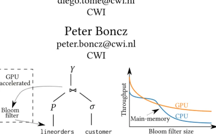
Figure 1: Early pruning in large selective joins

CPUs, these devices include GPUs, FPGAs and specialized hardware. Particularly, the acceleration of compute-intensive tasks [20] using GPUs has gained tremendous traction.

GPUs significantly outperform CPUs in compute-intensive tasks, as they combine a massively parallel architecture with high bandwidth memory. However, since analytic workloads are data-intensive rather than compute-intensive, GPUs typ-ically fail to accelerate database workloads. The main prob-lems are the limited size of the local GPU memory and the limited PCI bus bandwidth between CPU and GPU. GPUs typically have less than 16 GiB of memory, while main mem-ories attached to a CPU are typically an order of magnitude larger (and flash or other persistent memories are yet an-other order of magnitude bigger). The current generation of bus architectures in practice is limited to sustained transfer of 12 GiB/s; whereas CPU memory bandwidth is well over 100 GiB/s and internal GPU memory can be over 400 GiB/s. In scientific literature where advances of GPU-accelerated database systems are demonstrated, the experiments are typ-ically performed on small datasets, cached in the local GPU memory, such that significant CPU-GPU data transfers are avoided; or the CPU baselines that are compared with are not state-of-the-art systems (e.g. VectorWise [3, 23] or Hy-per [17, 19] would qualify our definition). While there are a few start-up companies with GPU-accelerated database solu-tions, these have little traction yet in the industry – a far cry from the situation in Machine Learning (ML) where GPUs are in extreme demand by industry (ML being a compute rather than data-intensive workload). Given that heteroge-neous hardware acceleration would be especially useful for Big Data analysis tasks where queries take a lot of time, the search was still on for database use-cases where GPUs fit in.

(2)

This paper contributes a use-case where GPUs can truly contribute: early pruning in large selective joins.

Recent work [13] shows that GPUs are able to efficiently prune using Bloom filters [2]. In database systems, Bloom filters can be exploited in queries with selective joins, to quickly eliminate disqualifying tuples, before they even en-ter the join. Concretely, afen-ter completing the build phase of a hash-join, a bloom filter can be created that holds the set of keys in the hash table. This Bloom filter is smaller than the hash table and is cheaper to probe. Also, it can be probed very early in the query (early pruning) even in the scan operator on the probe side of the query plan. This could mean that when whole stretches of keys fail to qualify, whole blocks of data holding the non-key columns can be skipped (saving I/O and decompression effort in column stores). Also, other operators in between the scan and the selective join (e.g., other joins or aggregations) will receive less tuples and will be accelerated, thanks to the early pruning. This is depicted in the left of Figure 1. However, large hash tables that hold many keys require larger Bloom filters. Once the Bloom fil-ter size exceeds CPU caches, L3 cache size in particular, the Bloom filter lookup throughput drops significantly due to additional main memory access. The right side of Figure 1 illustrates that this is a situation where the higher memory bandwidth of GPUs will significantly improve lookup per-formance. A Bloom filter is much smaller than a hash table storing the same amount of keys and some payloads – there-fore it is reasonable that to assume that if a hash table fits in the CPU memory, the corresponding Bloom filter should fit in GPU memory. GPUs are more powerful than CPUs for computing hash functions needed in Bloom filter tests, have a local memory with significantly more random-access bandwidth than the CPU, and since only keys (or extracts thereof) have to be moved to the GPU, data transfers over the bus are relatively small. All of this makes CPU offloading of large Bloom filtering a very promising task. Our micro-benchmarks show that raw Bloom filter lookups are up to 6×faster on the GPU than on the CPU in case the Bloom filter is larger than the CPU cache (skip to Figure 3).

The follow-up question is what a database architecture should look like that can efficiently offload tasks to the GPU. On the one hand, it has been shown that many-core CPUs can perfectly scale joins using shared hash-tables and an adaptive, fine-grained ("morsel driven") task allocation [17]. On the other hand, for Bloom filtering, keys needs to be transferred to the GPU on-the-fly; and these transfers have to be relatively coarse-grained in order to achieve good transfer speeds over the bus. Given the fact that bus transfer speeds are a bottleneck (an order of magnitude slower than memory access), this is a critical detail. We therefore propose thefluid

co-processing framework, wherein (i) query pipelines are cut into dependent fragments that may run on a specific

Bloom filter Lookup/ ... ... Word Insert (a) Traditional Bloom filter Lookup/ ... ... Block Sector ... Word Insert

(b) Blocked & Sectorized [15]

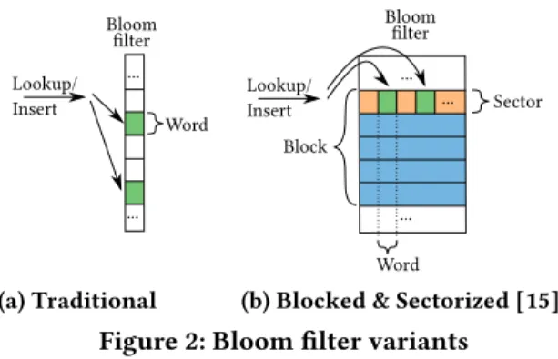
Figure 2: Bloom filter variants

device or on both (ii) both CPU and GPU adaptively accept work from a shared queue and (iii) different granularities (amounts of tuples) are used for work-distribution: the GPU getting larger work units at-a-time than the CPU. Our early results show that fluid co-processing consistently improves end-to-end CPU performance of early pruning in join queries thanks to the GPU, by factors up to 2-3×.

2 FAST CPU AND GPU BLOOM FILTERS

The Bloom filter [2] represents a collection ofnkeys with an initially-zeroed array ofmbits, setting for each inserted keykbits to 1, using as many hash functions to identify the positions [0,m) where the bits are set in the array. This struc-ture allows for fast true-negative tests, but it can produce false-positives at some probability that drops with larger mandk. In their classic implementation, multiple (up tok) random memory accesses are necessary to check the bits a key sets. AblockedBloom filter [21] represents the data structure as a set ofm/Bblocks, each of which contains a small Bloom filter of sizeB– a hash function determines in which block a key must be stored. To optimize in-memory processing, the size of a block is equal to the the size of a cache line, because this allows a key to be looked up with at most one cache miss. On GPUs, cache lines are typically 128 bytes and aligned in global memory; we therefore use up to B=1024 bits in our blocked GPU Bloom Filters.

Recently, an experimental study was published on (CPU-based) Bloom filtering [15], which also introduced a number of innovations. One of these is the idea to use minuscule blocks that are as small as a 32-bit register, because this allows to test allkbits in one load-compare instruction se-quence. That is, the lookup code first computes a bit mask withk bits set, loads one word and tests that against the mask with one AND and on CMP instruction. Rather than requiringk independent hash calculations, it can often do with a single 64-bits hash, extracting from that a sequence ofloд2(B) bits to identify the block, andk small (5-bit =

loд2(32)) random bit sequences to identify the bits. Such register-blocked Bloom filters test all bits at once, as opposed to classic Bloom filters which need a loop withkiterations,

(3)

1 4 16 64 256 Bloom filter size (MiB)

1000 300 400 500 600 700 800 900 2000 3000 4000 5000 6000 7000 Thr oughput (MPr ob e/s) 6x CPU GPU

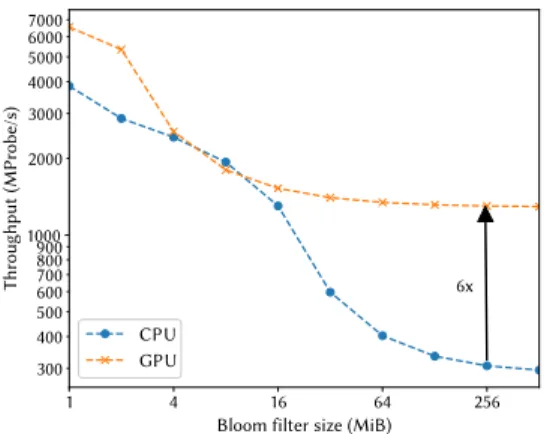
Figure 3: Bloom filter probe throughput varying the bloom filter size. For larger Bloom filters, the

through-put on GPU is up to 6×the CPU lookup performance.

This allows efficient support of (a) larger inner rela-tions (hence, bigger Bloom filters) and/or (b) more pre-cise Bloom filters.

with an early-out if a bit is found to be 0. Getting rid of the loop and early-out branch is actually beneficial for the GPU, because control-divergence is avoided.

Register-blocked Bloom filters are quite radical as they maximally reduce computational work, but this goes at the expense of accuracy; because mini Bloom filters of just 32 bits can get unlucky and receive many keys, in which case their selective power deteriorates. In order to use larger blocks that occupy the full 1024 bits of a GPU cache-line (or 512-bits in case of the CPU), one can divide the block in multiplesectors, e.g. 32 sectors of 32-bits. Thesectorized

Bloom filter (see Figure 2) still tests multiple bits in each sector at once to reap the aforementioned computational benefits; but, it evenly spreads thek-bits over multiple sectors in the block. In fact, not all sectors need to receive bits; rather, a few of them are selected with yet another few random bits from the hash number. For instance withk=8, one could set/test 4 bits concentrated in two 32-bits words (=sectors) out of 32. This approach thus combines computational and memory efficiency, and can achieve high-precision and very low lookup latency [15].

Figure 3 shows micro-benchmarks of our C++ and CUDA implementation of Bloom filters on GPUs and CPUs (k=2, n/m=8) for varying Bloom filter sizes (m). The hardware is described in Section 4. For fairness, the CPU uses all its cores; and the GPU performance includes copying the keys (input) and the boolean results (output) resp. from and to CPU memory. In all, while the CPU is competitive with the GPU for smaller Bloom filters; when they start to exceed the CPU L3 cache (beyond 16 MiB), a large performance gap widens, up to a factor 6×. GPU morsel CPU morsel CPU morsel Hash Table GPU morsel GPU+CPU Worker Bloom Filter Bloom Filter

CPU Worker CPU Worker Table GPU

Bitmap accelerated

Figure 4: Fluid Co-Processing allows dynamic offload-ing through work-stealoffload-ing

3 FLUID CO-PROCESSING

Commonly, co-processing approaches statically assign spe-cific operations to devices. Notable examples are CoGaDB [5] and HAPE [7]. CoGaDB allows offloading specific operators to devices. HAPE relies on HetExchange [6], an extension of Volcano-modelexchangeoperators [9] that allow offloading of complete pipelines. However, static resource allocation has two well-known caveats:

(a) It requiresaccurate cost-modelsto decide what to of-fload. In practice, building “good” cost-models is very hard and cost-models very often not precise [18].

(b) Optimal parallel performance requiresload-balance, or available hardware will become under-utilized. Imbalance can have many causes, e.g. by interference (another process running, processors clocking up/down), sub-optimal data distributions or different hardware characteristics. However, once a static parallel plan is created, load-balancing is hard to achieve [10, 17].

3.1 Morsel-driven Parallelism is not enough

For CPU-only systems, morsel-driven parallelism [17] is known to eliminate, or at least mitigate, these issues. In a morsel-driven system, workers repeatedly consume tasks from a global queue and execute them. The task granularity, the morsel size, leads to the trade-off between scheduling overhead (removing tasks from a queue) and load-balancing. Small morsel sizes will lead to high scheduling overhead whereas large morsel sizes will severely worsen opportuni-ties for load-balancing.

However, extending the traditional morsel-driven paral-lelism into a co-processing system is more complex:

(a) The optimal unit of work - the morsel size - differs from device to device. For parallel CPU-based systems Leis

(4)

S t r e a m s t r e a m ;

w h i l e ( ! done ) { Range r a n g e ;

i f ( p r o b e . i s _ g p u _ d o n e ) {

/ / Consume r a n g e o f Bloom f i l t e r r e s u l t and j o i n them

i f ( g e t _ r a n g e ( r a n g e , s t r e a m , c p u _ m o r s e l _ s i z e ) ) { j o i n ( s t r e a m , r a n g e ) ; i f ( l a s t _ m o r s e l ) { s t r e a m . i s _ c p u _ d o n e = t r u e; } } } i f ( s t r e a m . i s _ c p u _ d o n e ) { / / S c h e d u l e new GPU p r o b e s t r e a m . r e s e t ( ) ; s t r e a m . i s _ g p u _ d o n e = f a l s e; s t r e a m . i s _ c p u _ d o n e = f a l s e; i f ( g e t _ r a n g e ( r a n g e , t a b l e , g p u _ m o r s e l _ s i z e ) ) { s t r e a m . s c h e d u l e ( r a n g e ) ; } } / / F a l l b a c k : CPU work i f ( g e t _ r a n g e ( r a n g e , t a b l e , c p u _ m o r s e l _ s i z e ) ) { c p u _ p i p e l i n e ( t a b l e , r a n g e ) ; } }

Listing 1: Simplified GPU+CPU worker loop with one probe stream (probe)

et al. [17] suggest morsel sizes of roughly 10K – 100K. CPU-GPU communication latencies force 10×– 100×larger morsel sizes, to minimize scheduling overheads and achieve efficient data transfers. The absence of an efficient common morsel size prevents the naive approach of dividing the work into equally sized chunks and pushing them into a queue.

(b) The classical morsel-driven parallelism executes a query pipeline-by-pipeline. However, for co-processing, a pipeline can contain multiple pipelinefragments. When executing our join query on the GPU, we have two such fragments: The first fragment, scans the table and evaluates the Bloom filter on GPU. As we want to parallelize the following join processing, we need a second fragment which consumes morsels from the Bloom filter results and executes the join followed by the aggregation.

Because of these reasons, we concluded that plain morsel-driven parallelism is not “good” enough for Co-Processing and therefore we needed to extend it.

3.2 Fluid Parallelism for Co-processing

To allow multiple morsel sizes, we replaced the task queue (morsel queue) with a lock- and wait-free linear allocator. It works similar to the following pseudo-code:

b o o l g e t _ r a n g e ( Range& out , c o n s t T a b l e& t , i n t m o r s e l _ s i z e ) { o f f s e t = _ _ s y n c _ a d d _ a n d _ f e t c h (& t . c u r r e n t _ o f f s e t , m o r s e l _ s i z e ) ; i f ( o f f s e t > t . s i z e ( ) ) r e t u r n f a l s e; / / f a i l e d g e t t i n g r a n g e / / u s e up t o ' m o r s e l _ s i z e ' s t a r t i n g from o f f s e t o u t . o f f s e t = o f f s e t ; o u t . num = MIN ( t . s i z e ( ) − o f f s e t , m o r s e l _ s i z e ) ; r e t u r n t r u e; }

The allocator returns a range which points into the table t. The linear range allocation relies on the atomic increment (__sync_add_and_fetch) to move the starting offset forward. If a valid offset was allocated, the actual size of the morsel is determined. In practice, all morsels, except the last one, will have the givenmorsel_size.

In contrast to morsel-driven parallelism’s one active line, co-processing can work with multiple alternative pipe-lines. In our case study, we have (1) the whole CPU-only Bloom-filter + join-probe + aggregation pipeline that starts with CPU Bloom filtering, (2a) GPU Bloom filtering and (2b) CPU join-probe + aggregation. Tuples are either processed with (1) or by (2a) followed by (2b). Figure 4 illustrates our framework. Generally, we differentiate betweenGPU+CPU

workers andCPU workers. Their main difference being that GPU+CPU workers can also schedule GPU work whereas CPU workers only operate on CPU-only pipeline fragments.

ACPU workerruns in a loop. In each iteration it will try to consume a morsel that either (a) evaluates the full pipeline for a whole CPU morsel or, if a GPU bloom filter probe is ready, (b) using the GPU bloom filter result disqualify non-matching tuples and execute the join.GPU+CPU workersextend CPU workers with the ability to also handle GPU work. They run a loop similar to the pseudo-code in Listing 1. To allow full utilization of the GPU, we prioritize GPU work over CPU work. Additionally, we allow the use of multiplestreams. Each stream consists of copying to the GPU, executing the Bloom filter lookup kernel and copying the results back. Using multiple streams allows the GPU to efficiently overlap computation kernels and data movement.

If a free/idle GPU stream is detected, it will first try to consume a large GPU morsel from the table and schedule an-other GPU Bloom filter probe. This probing process will run asynchronously and is handled by the CUDA implementa-tion. While the GPU+CPU worker waits for a probe to finish, it will execute regular CPU work. When a GPU Bloom filter lookup is finished, it will be schedule for work-sharing i.e. we add it to a global queue of finished probes from which CPU and GPU+CPU workers can consume morsels and execute the remaining pipeline fragment.

4 EXPERIMENTAL EVALUATION

We implemented the proposed techniques in a prototype

1_{which evaluates the query:}_{SELECT SUM(a.k), SUM(b.p1),}

SUM(b.p2), ..., SUM(b.p32) FROM a, b WHERE a.k = b.k. In detail, our prototype operates on cache-resident vectors in a columnar fashion, so called "vectorized execution" [3]. Its join operator executes a flat, non-partitioned, primary-key-foreign-key hash join (i.e. either zero or one match in

1_{Source code can be found under: https://github.com/t1mm3/fluid_}

(5)

0 10 20 30 40 50 60 70 Selectivity (in %) 2 4 6 8 10 12 14 Time (in s) CPU, no BF CPU, BF GPU+CPU, BF GPU+CPU, BF (cached)

Figure 5: Co-processing always wins (64 MiB Bloom filter). Lower selectivity means more pruned tuples.

the hash table) on a bucket-chained hash table with records in row-wise layout [22]. Additionally, we simulated an ex-pensive operator (Pin Figure 1) between scan and join. In our experiments, we use a Bloom filter with one sector and setk =2 bits. We used a probe relation with a cardinality of 1 billion tuples. However, when scaling the inner rela-tion we increased the outer relarela-tion to 4 billion tuples. Our co-processing framework uses 4 GPU streams and morsel sizes of 16 Ki tuples for CPU and 1 Mi tuples for GPU. Our experiments were conducted on a 10-core i9-7900X with 13.75 MiB L3 cache and 32 GiB main-memory. We always use all 10 cores. As GPU, we used one GeForce GTX 1080 with 8 GiB memory. We used Fedora 28 with CUDA 10.1 and driver version 418.56.

In this section, we first evaluate the performance of our fluid co-processing framework. Afterwards, we investigate the influence of a varying pipeline costcPand cardinality of

the inner relation on the query time, followed by a discussion of the influence of the number of streams on the performance. Last but not least, we discuss the scheduling behaviour of

ourfluidco-processing framework.

4.1 Fluid Co-Processed Join

The effectiveness of early pruning depends on the selectivity of the join itself. The more tuples eliminated by the join, the more effectively can a Bloom filter prune them already in the scan. Therefore, we evaluated the overall performance of the join (probe) pipeline over varying selectivity. Figure 5 visualizes our results.

We noticed that, during CPU-only execution (CPU, BF) the benefit of using the Bloom filter to prune is limited, compared to CPU-only execution without a Bloom filter (CPU, no BF). This is due to the size of the Bloom filter. As the Bloom filter exceeds the CPU caches, it introduces additional cache misses and put further stress on the memory subsystem. With rising

0 10 20 30 40 50 60 70 Selectivity (in %) 500 600 700 800 900 1000 1100 1200 Join pr ob e time (in cy cles/tuple) CPU, BF GPU+CPU, BF GPU+CPU, BF (cached)

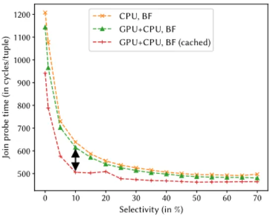
Figure 6: GPU+CPU joins are faster but CPU-GPU data transfers appear to slow joins down. Depicted is only (per-tuple) join time for surviving tuples. With low se-lectivities, join time is less important for query time and it spikes due to small vector overhead.

selectivity (less tuples pruned) the benefit of early filtering goes to zero and only the filtering overhead, additional cache misses in particular, remains.

The GPU+CPU execution (GPU+CPU, BF), however, ben-efits from the GPU’s additional computational power and memory bandwidth. For low selectivities this leads to a per-formance improvement up to 3×compared to the non-Bloom CPU implementation and roughly 2×compared to the CPU-only version. With rising selectivity, similar to the CPU-CPU-only scenario, the benefit of early pruning gradually disappears. However, the risk of slowing down the join is much lower because the Bloom filter is much faster i.e. it uses CPU and GPU in parallel.

We now focus on the performance of the join. Figure 6 displays the join time with the probe key columnalready

re-sidingin the GPU memory (GPU+CPU, BF (cached)). Caching

the keys speeds up the GPU pipeline (Bloom filter and send-ing results back) which, in turn allows more tuples to be processed on GPU. This leads to a significant speedup of up to 27% which additionally boost the already existing perfor-mance gain. However, caching the keys only allows the GPU to consume≈ 5% more tuples (Figure 8) and is therefore not explaining the 27% boost (the lion’s share, 95%, did not change). This indicates that the memory transfer from CPU to GPU (HtoD) and back (DtoH) isnot freeand affects the memory bandwidth of the host (CPU).

4.2 Scaling Pipeline Cost and Inner Relation

In joins, the efficiency of early pruning using Bloom depends on a variety of factors: (a) the size of the inner (build) relation, (b) the size of the Bloom filter, (c) the number of hash func-tionsk, (d) the Bloom filter type (naive, blocked, counting etc.) and (e) cost of the pipelinecP.

(6)

Additional Pipeline CostcA

Inner

Relation

Size

0 50 100 200 400 800

512 Mi n/a n/a (2 Gi, 3) (2 Gi, 3) (4 Gi, 6) (4 Gi, 6)

256 Mi n/a n/a (2 Gi, 6) (2 Gi, 6) (2 Gi, 6) (2 Gi, 4)

128 Mi n/a (512 Mi, 2) (1 Gi, 4) (1 Gi, 4) (2 Gi, 6) (2 Gi, 6)

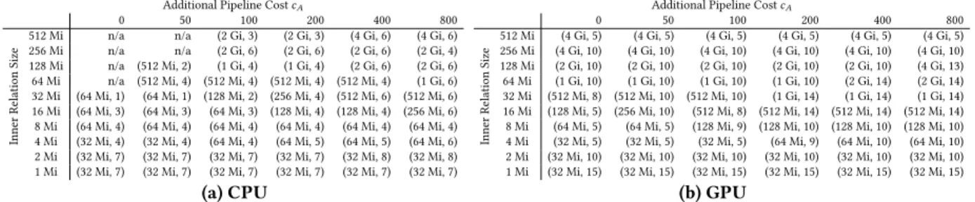
64 Mi n/a (512 Mi, 4) (512 Mi, 4) (512 Mi, 4) (512 Mi, 4) (1 Gi, 6) 32 Mi (64 Mi, 1) (64 Mi, 1) (128 Mi, 2) (256 Mi, 4) (512 Mi, 6) (512 Mi, 6) 16 Mi (64 Mi, 3) (64 Mi, 3) (64 Mi, 3) (128 Mi, 4) (128 Mi, 4) (256 Mi, 6) 8 Mi (64 Mi, 4) (64 Mi, 4) (64 Mi, 4) (64 Mi, 4) (64 Mi, 4) (64 Mi, 4) 4 Mi (32 Mi, 4) (32 Mi, 4) (64 Mi, 4) (64 Mi, 5) (64 Mi, 5) (64 Mi, 6) 2 Mi (32 Mi, 7) (32 Mi, 7) (32 Mi, 7) (32 Mi, 7) (32 Mi, 8) (32 Mi, 8) 1 Mi (32 Mi, 7) (32 Mi, 7) (32 Mi, 7) (32 Mi, 7) (32 Mi, 7) (32 Mi, 7)

(a) CPU

Inner

Relation

Size

0 50 100 200 400 800

512 Mi (4 Gi, 5) (4 Gi, 5) (4 Gi, 5) (4 Gi, 5) (4 Gi, 5) (4 Gi, 5)

256 Mi (4 Gi, 10) (4 Gi, 10) (4 Gi, 10) (4 Gi, 10) (4 Gi, 10) (4 Gi, 10) 128 Mi (2 Gi, 10) (2 Gi, 10) (2 Gi, 10) (2 Gi, 10) (2 Gi, 10) (4 Gi, 13) 64 Mi (1 Gi, 10) (1 Gi, 10) (1 Gi, 10) (1 Gi, 10) (2 Gi, 14) (2 Gi, 14) 32 Mi (512 Mi, 8) (512 Mi, 10) (512 Mi, 10) (1 Gi, 14) (1 Gi, 14) (1 Gi, 14) 16 Mi (128 Mi, 5) (256 Mi, 10) (512 Mi, 8) (512 Mi, 14) (512 Mi, 14) (512 Mi, 14) 8 Mi (64 Mi, 5) (64 Mi, 5) (128 Mi, 9) (128 Mi, 10) (128 Mi, 10) (128 Mi, 10) 4 Mi (32 Mi, 5) (32 Mi, 5) (32 Mi, 5) (64 Mi, 9) (64 Mi, 10) (64 Mi, 10) 2 Mi (32 Mi, 10) (32 Mi, 10) (32 Mi, 10) (32 Mi, 10) (32 Mi, 10) (32 Mi, 10) 1 Mi (32 Mi, 15) (32 Mi, 15) (32 Mi, 15) (32 Mi, 15) (32 Mi, 15) (32 Mi, 15)

(b) GPU

Table 1: Performance-optimal Bloom filter configurations (m,k) for combinations of inner relation cardinality

and additional pipeline costcAwith Bloom filter sizem(bits) andk hash functions. GPU Bloom filters efficiently

support larger filters with more hash functions (k up to 14-15) than CPU Bloom filters.

Inner Relation Size 0 50 100 200 400 800 512 Mi n/a n/a 14.8% 14.8% 2.8% 2.8% 256 Mi n/a n/a 2.8% 2.8% 2.8% 2.7% 128 Mi n/a 15.6% 2.7% 2.7% 0.2% 0.2% 64 Mi n/a 2.7% 2.7% 2.7% 2.7% 0.2% 32 Mi 39.3% 39.3% 15.5% 2.7% 0.2% 0.2% 16 Mi 16.1% 16.1% 16.1% 2.7% 2.7% 0.2% 8 Mi 4.1% 4.1% 4.1% 2.7% 2.7% 2.7% 4 Mi 4.1% 4.1% 0.8% 0.8% 0.8% 0.2% 2 Mi 0.8% 0.8% 0.8% 0.8% 0.2% 0.2% 1 Mi 0.1% 0.1% 0.1% 0.1% 0.1% 0.1% (a) CPU

Inner Relation Size 0 50 100 200 400 800 512 Mi 2.3% 2.3% 2.3% 2.2% 2.2% 2.2% 256 Mi 0.1% 0.1% 0.1% 0.1% 0.1% 0.1% 128 Mi 0.1% 0.1% 0.1% 0.1% 0.1% < 0.1% 64 Mi 0.1% 0.1% 0.1% 0.1% < 0.1% < 0.1% 32 Mi 0.1% 0.1% 0.1% < 0.1% < 0.1% < 0.1% 16 Mi 2.3% 0.1% < 0.1% < 0.1% < 0.1% < 0.1% 8 Mi 2.3% 2.3% 0.1% 0.1% 0.1% 0.1% 4 Mi 2.3% 2.3% 2.3% 0.1% 0.1% 0.1% 2 Mi 0.1% 0.1% 0.1% 0.1% 0.1% 0.1% 1 Mi < 0.1% < 0.1% < 0.1% < 0.1% < 0.1% < 0.1% (b) GPU

Table 2: Performance-optimal Bloom filter false-positive ratio (accuracy) for combinations of inner relation

car-dinality and additional pipeline costcA - corresponding to the configurations in Table 1. Performance-optimal

GPU Bloom filters achieve a higher accuracy than CPU Bloom filters. Higher additional pipeline costcAleads to

more accurate Bloom filters.

0 50 100 200 400 800 Additional Pipeline CostcA 1 2 4 8 16 32 64 128 256 512 Inner Relation Car dinality (MiT uples)

(a) CPU-only Bloom filter

0 50 100 200 400 800 Additional Pipeline CostcA

2.5 5.0 7.5 10.0 12.5 15.0 17.5 20.0

(b) GPU+CPU Bloom filter

Figure 7: Influence of inner relation’s cardinality and pipeline costcP on query time at 1% selectivity. Col-ors represent the total runtime (s). Variations in cP

are simulated through an additional pipeline costcA.

Bloom filters on GPU allow to accelerate the upper half (large inner relations) and are able to speed up expensive pipelines (highcP).

In this experiment, we demonstrate the effects of the pipe-line costcP and inner relation size on the run time. For

each combination of CPU/GPU, inner relation andcP, we

determined the performance-optimal Bloom filter, as defined by Lang et al. [15], using a hardware-calibrated cost-model. Note that a Bloom filter might not always provide a benefit. In particular, a combination of a smallcPand an expensive

Bloom filter might lead to inferior performance. We marked such cases as invalid values.

Bloom Filter Configurations & Accuracy. Using the

cost-model, we obtained performance-optimal Bloom filter con-figurations for a variety of inner relational cardinalities (i.e., join build sizen) and pipeline cost. For the latter, we increase the basic scan-filter-join costcPby adding an additional cost

cAthat corresponds to operators (such as aggregations or

other joins) that would be in between the scan-filter and the join. The Bloom filter sizemand the number of hash functionskfor each filter is shown in Table 1. We noticed that, compared to the CPU, the GPU efficiently allows larger Bloom filters and roughly 2×more hash functions. On the CPU, such configurations would suffer from low memory throughput and high computational cost for the hashing.

The false-positive ratiof of each filter is depicted in Ta-ble 2. With increasing pipeline cost, highercA, we noticed

a trend to higher accuracy. The reason is that, with a high penalty for a false-positive, it makes more sense to pay the

(7)

price of a more expensive Bloom filter with higher precision to prevent many false-positives.

Compared to CPU Bloom filters, GPU Bloom filters tend to have a very low false-positive ratio because (a) the GPU has a higher memory bandwidth (less penalty for larger filters) and (b) more computational power - hence a GPU can compute more hash functions than a CPU, before becoming compute-bound rather than memory-compute-bound. A configuration with size m=4GB andk=14 hash functions is not practical on a CPU, but can be performance-optimal on a GPU.

Bloom Filter Lookup Performance.After determining the

optimal Bloom filters, we ran the experiment. Figure 7 vi-sualizes our results. The lookup performance of CPU-only Bloom filters, as visible in Figure 7a, is more sensitive to the size of the build relation i.e. fast lookup is only achieved for Bloom filters that fit into cache. Consequently, the benefits of early pruning decreases with the Bloom filter size, as the lookup becomes more expensive with increasing build sizes.

In contrast to CPU-only filtering, the GPU+CPU Bloom filtering (see Figure 7b) is much less sensitive to the build size, and consequently the Bloom filter. This allows efficient pruning in selective joins even for large dimension tables (i.e. larger inner relations).

Higher pipeline costs (cP+cA) tend to justify more

accu-rate Bloom filters. The early pruning becomes more costly in more accurate filters, but if offset by the much more expen-sive pipeline cost, that can be saved for every pruned tuple. We notice again that the overhead of more accurate Bloom filters on GPU+CPU ismuchlower than on CPU and, hence, allows much more effective pruning.

4.3 Optimal Number of Streams

In our fluid co-processing, the termstreamrefers to a work queue, where the CPU enqueues tasks for the GPU, such as kernel executions and memory transfers from the host to the device (HtoD) or from the device back to the hosts memory (DtoH). Modern GPUs are capable of performing two simultaneous (DMA) memory transfers, one in each direction. At the same time the GPU can execute kernels. Due to the fact that the streams are processed sequentially, a co-processing system needs multiple concurrent streams, associated with the same GPU, to overlap memory transfers and kernel execution and thus to maximize performance. In our query, each stream delivers tuples to the GPU, probes the Bloom filter, and sends the resulting bitmap back to the host memory. We aim to find the lowest number of streams which (a) keeps the GPU busy and (b) leads to the lowest run time. Therefore, we executed our co-processed join query with a selectivity of 1% on 1 billion tuples and measured the fraction of tuples sent to the GPU (GPU Utilization), as well as the runtime of the probe pipeline.

0 20 40 60 Selectivity (in %) 40 50 60 70 80 90 100 GP U Utilization (in %) 1 Stream 2 Streams 4 Streams 8 Streams

(a) ... when transferring keys

0 20 40 60 Selectivity (in %) 40 50 60 70 80 90 100 GP U Utilization (in %) 1 Stream 2 Streams 4 Streams 8 Streams

(b) ... when keys are cached

Figure 8: More than 4 streams do not provide a better GPU utilization. 0 20 40 60 Selectivity (in %) 2 4 6 8 10 12 Time (in s) 1 Stream 2 Streams 4 Streams 8 Streams

(a) ... when transferring keys

0 20 40 60 Selectivity (in %) 2 4 6 8 10 Time (in s) 1 Stream 2 Streams 4 Streams 8 Streams

(b) ... when keys are cached

Figure 9: Influence of more than 2 streams onto total query runtime is negligible.

GPU Utilization.The results are visualized in Figure 8a.

We noticed that GPU utilization heavily depends on the num-ber of streams. For only one stream, we can only filter up to≈80% of the tuples on the faster device (the GPU) and, hence, leave resources idle. With lower selectivities this ef-fect is more extreme. However, with more than 2 streams we noticed that almost all (> 98%) are being filtered by the GPU. When using 4 or 8 streams, we observed a better be-haviour for lower selectivities (≤5%). However, for higher selectivities we measured a degraded utilization. This indi-cates that, besides memory footprint, there is also CUDA overhead involved. We also noticed that using more streams are not necessarily the better choice for GPU utilization, as compared to using 4 streams, 8 streams lead to inferior GPU utilization. We argue that, in our case, 4 streams appears to be the optimal choice, as it provides high GPU utilization for low selectivities, as well as, negligible degradation for high selectivites.

When the keys are cached on the GPU, see Figure 8b, we noticed similar behaviour. However, as the keys do not need to be transferred to the GPU (i.e. GPU kernels are faster), we measured slightly higher GPU utilization.

Runtime.In Figure 9 we plotted the runtime of the probe

pipeline with a given number of streams. For 1 stream, we observed a penalty because the GPU is not fully utilized. For 2 or more streams, we did not notice any significantly

(8)

128Ki 1 Mi 16Mi 128Mi

GPU morsel size 16 Ki 128 Ki 1 Mi CP U morsel size 2.2 2.4 2.6 2.8 3.0 3.2 3.4

Figure 10: Total runtime (s) w.r.t. morsel sizes. Large morsels worsen load-balancing and leave resources idle. Small GPU morsels lead to additional overhead.

improved runtime. Hence, for query runtime 2 to 4 streams appear to be the optimal choice.

Optimal number of steams.We found that more (than 4)

streams neither improve query performance nor GPU uti-lization. As each stream materializes part of the relation, the memory footprint scales with the number streams and, hence, a high number of streams will inflate the footprint of the query. Therefore, we conclude that 2 to 4 streams are enough to (a) keep the GPU busy and (b) lead to the optimal runtime.

4.4 Optimal Morsel Sizes

The performance of our fluid co-processing strongly depends on the morsel sizes used for CPU and GPU work. The choice of morsel sizes is typically a trade-off between load-balancing behaviour and scheduling overhead as small morsels lead to good load balance between workers but higher scheduling overhead, and vice versa. Hence, the optimal morsel sizes is the smallest one which still allows efficient execution. We, therefore, experiment with various combinations of morsel sizes for CPU and GPU. Our results can be seen in Figure 10.

We noticed that too small CPU morsels increase total run-time as they incur higher scheduling overhead. Too large CPU morsels also increase the runtime as they leave re-sources idle (most workers are done whereas the last ones are still processing their large morsels). Similarly we noticed a tendency that small GPU morsels incur additional schedul-ing and GPU-specific overhead, i.e. GPU-internal schedulschedul-ing and less efficient data transfers lead to lower throughput. In the other extreme large GPU morsels fully utilize GPU resources but leave CPU resources idle.

We found that 16 Ki tuples for CPU and 1 Mi tuples for GPU are sufficient to allow efficient processing and are, there-fore, the optimal choice in our case.

4.5 Scheduling Behaviour

0 1 2 3 4 5 6 7 8

Time (in cycles) 1e9

W

orker

Post GPU Join CPU Bloom + Join Schedule GPU Probe

(a) 1% selectivity

0 1 2 3 4 5 6 7 8

W

orker

(b) 5% selectivity

0 1 2 3 4 5 6 7 8

W

orker

(c) 10% selectivity

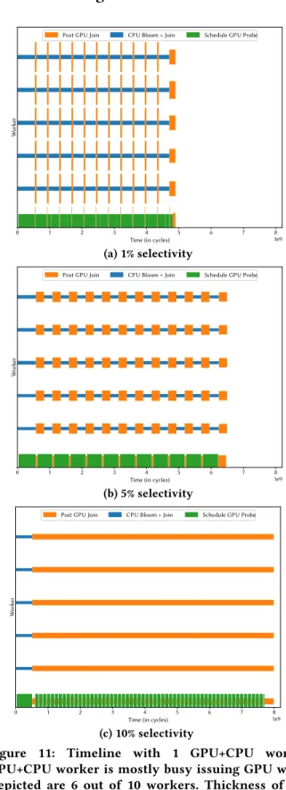
Figure 11: Timeline with 1 GPU+CPU worker. GPU+CPU worker is mostly busy issuing GPU work. Depicted are 6 out of 10 workers. Thickness of the barsPost GPU JoinandCPU Bloom + Join represents their processing speed (higher means faster).

(9)

0 1 2 3 4 5 6 7 8

W

orker

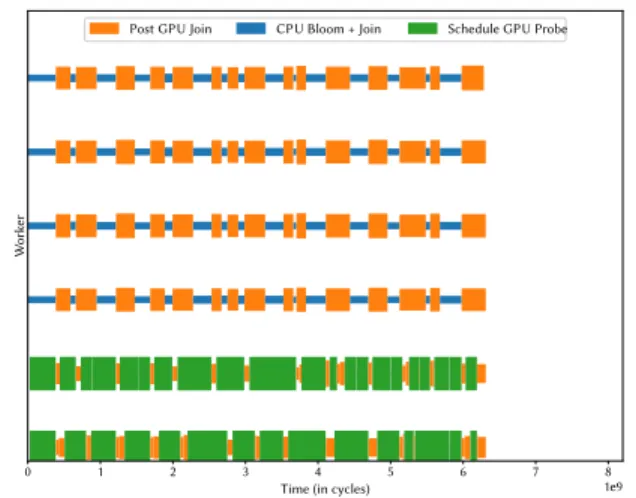
Figure 12: Timeline with 2 GPU+CPU workers with 5% selectivity. Scheduling GPU work is evenly distributed over the 2 worker threads. Depicted are 6 out of 10

workers. Thickness of the barsPost GPU JoinandCPU

Bloom + Joinrepresents their processing speed (higher means faster).

Our fluid co-processing schedules tasks dynamically. To give an insight into the scheduling decisions being made, we ran the same experiment as in Section 4.1, profiled scheduling decisions and plotted onto a timeline. First, we discuss the behaviour of our prototype with only 1 GPU+CPU worker and, afterwards, the behaviour with 2 GPU+CPU workers.

1 GPU+CPU Worker.We ran the experiment for three

dif-ferent selectivites (1%, 5% and 10%). Figure 11 visualizes the results we obtained. We noticed that the 1 GPU+CPU was mostly busy issuing GPU work (in the following experiment we parallelize this part using 2 GPU+CPU workers).

At 1% selectivity (Figure 11a), we observed that most time is spent on theCPU Bloom + Join. The reason is that the GPU-accelerated pipeline (Post GPU Join) runs in negligible time as it eliminates 99% of tuples in a very lightweight fashion. The remaining time each worker is trying to prevent going idle by "stealing" CPU morsels and executing the CPU-only pipeline.

When moving to 5% selectivity (Figure 11b), we found that there is roughly an equal amount of time spent on the GPU-accelerated and the CPU-only pipeline.

Moving to 10% selectivity (Figure 11c), we observe the opposite of the 1% case: Most time is spent on the GPU-accelerated Join (Post GPU Join) because the join, includ-ing fetchinclud-ing payloads, is very expensive. However, we also noticed astartup lagfor the GPU-accelerated Join. This is caused by the initial latency of issuing GPU work until the results from the GPU are received.

2 GPU+CPU Workers.In the previous experiment, it

ap-peared that the one single GPU+CPU worker might be over-loaded. Therefore, we modified the experiment and paral-lelize issuing GPU work over 2 GPU+CPU workers which can concurrently schedule GPU work. The results can be seen in Figure 12. We noticed that allowing multiple GPU+CPU workers tends to worsen initial load-balance (at the start of the query). The cause of this behaviour is the preference of GPU+CPU workers to issue GPU work. When creating GPU+CPU workers, each will first schedule GPU work which involves locking inside the CUDA library. However, we want to highlight, that our fluid co-processing framework is still able to achieve load-balance and, hence, the negative influ-ence of such delayed starts, or other interferinflu-ence, is signifi-cantly reduced.

5 RELATED WORK

Co-processing can be seen as an intra-query parallelization problem where different devices work together. Many data-base systems use Volcano parallelism [9] to adapt to modern multi-core hardware. Notable examples are SQLServer [16], Oracle [14] and Vectorwise [23]. Recently, it found applica-tion in Co-processing, as HetExchange [6] which allows to offload whole pipelines. Volcano originally became popular because it allowed an easy integration of parallelism into existing single-threaded systems by abstracting the paral-lelization intoExchangeoperators. This also means that paral-lelization and partitioning decisions have to be made at query optimization time rather than dynamically at query runtime. This, consequently, creates imbalance between threads and leaves resources idle. These issues have been fixed through dynamic morsel-driven parallelism [17]. It splits table ranges into tasks. These tasks are inserted into a global queue from which multiple workers can consume and process this task. Recently, a dynamic virtual machine architecture was pro-posed to allow cross-device load-balancing [10]. This idea inspired our fluid co-processing framework to perform adap-tive work placements for different devices, but instead of placing the work on the unit, here we adapt the granularity of work per device.

A number of GPU co-processing database systems have been developed, most notably Ocelot [12], CoGaDB [5] and HAPE [7]. Ocelot was proposed as a hardware-oblivious data-base engine to abstract away operators from CPU and GPU devices [12]. CoGaDB [5] places operators on devices at run-time, and allows pipeline parallelism. However, compared to our Fluid Co-processing, CoGaDB’s operator placement is neither fully dynamic, nor elastic. HAPE [7] is based on HetExchange [6]. Entire pipelines are compiled for different architectures (CPUs and GPUs). Thereby, CPUs and GPUs perform the same tasks and Exchange operators “route” the

(10)

tuples between the executing devices. In contrast, our pro-totype offloads different tasks (i.e. Bloom filter probe) to a different device, that eventually assists query execution on the CPU which leads to fully dynamic partitioning.

Our case study uses Bloom filters to accelerate selective joins. Bloom filters were introduced by Bloom [2]. Similar data-structures for approximate membership queries have been discovered. Notable examples are Quotient filters [1], Cuckoo filter [8] and Morton filters [4]. However their per-formance on GPU has not been studied deeply.

6 CONCLUSIONS & FUTURE WORK

This work (finally) identified in Early Pruning of Selective Joins using Bloom filters a relevant database workload where CPU database systems can be significantly accelerated by GPU co-processing. We realized this in a prototype of the dynamic, adaptive, heterogeneousFluid co-processing frame-work. This framework splits pipelines into pipeline frag-ments, such that a pipeline can be co-processed on different devices. It also allows multiple equivalent pipeline fragments to co-exist, so certain tuple ranges use a CPU-only pipeline, whereas others follow a CPU-GPU pipeline consisting of mul-tiple fragments. Its shared work queue is inspired by the elas-tic and dynamic co-processing model based of morsel-driven parallelism [17], but allows for different morsel granularities, tailored to each device. Note that the queue-based architec-ture also helps solve the problem of handling concurrent queries on a GPU, as the queue can coordinate scheduling of morsels belonging to different queries; and if the GPU is too busy, queries can just execute their morsels mostly (or completely) on the CPU-pipeline.

To measure the effectiveness of our techniques, we imple-mented a simple multi-threaded join query. Our experiments show performance improvements of up to 4×by dynamically offloading Bloom filtering.

In the future, we plan to deeply investigate the design space of GPU-based Bloom filtering; as our work so far just increases the Bloom filter block size to the correct GPU cache line size. We are experimenting with multiple GPU-specific Bloom filtering optimizations as well.

As for the Fluid Co-Processing framework, we intend to mature our prototype into a system that can execute generic and concurrent queries and perform adaptive offloading to heterogeneous hardware [11].

ACKNOWLEDGEMENTS

This work has been supported by the DFG project KE401/22.

REFERENCES

[1] M. A. Bender, M. Farach-Colton, R. Johnson, R. Kraner, B. C. Kuszmaul, D. Medjedovic, P. Montes, P. Shetty, R. P. Spillane, and E. Zadok. Don’t

thrash: how to cache your hash on flash. PVLDB, 5(11):1627–1637, 2012.

[2] B. H. Bloom. Space/time trade-offs in hash coding with allowable errors.Commun. ACM, 13(7):422–426, 1970.

[3] P. Boncz, M. Zukowski, and N. Nes. MonetDB/X100: Hyper-pipelining query execution. InCIDR, pages 225–237, 2005.

[4] A. D. Breslow and N. S. Jayasena. Morton filters: Faster, space-efficient cuckoo filters via biasing, compression, and decoupled logical sparsity. PVLDB, 11(9):1041–1055, 2018.

[5] S. Breß, H. Funke, and J. Teubner. Robust query processing in co-processor-accelerated databases. InSIGMOD, pages 1891–1906, 2016. [6] P. Chrysogelos, M. Karpathiotakis, R. Appuswamy, and A. Ailamaki. HetExchange: Encapsulating heterogeneous CPU-GPU parallelism in JIT compiled engines.PVLDB, 12(5):544–556, 2019.

[7] P. Chrysogelos, P. Sioulas, and A. Ailamaki. Hardware-conscious query processing in GPU-accelerated analytical engines. InCIDR, 2019. [8] B. Fan, D. G. Andersen, M. Kaminsky, and M. D. Mitzenmacher. Cuckoo

filter: Practically better than bloom. InCoNEXT, pages 75–88. ACM, 2014.

[9] G. Graefe. Encapsulation of parallelism in the volcano query processing system. InSIGMOD, pages 102–111, 1990.

[10] T. Gubner. Achieving many-core scalability in Vectorwise. Master’s thesis, Technical University of Ilmenau, 2014.

[11] T. Gubner. Designing an adaptive VM that combines vectorized and JIT execution on heterogeneous hardware. InProc. ICDE, 2018. [12] M. Heimel, M. Saecker, H. Pirk, S. Manegold, and V. Markl.

Hardware-oblivious parallelism for in-memory column-stores.PVLDB, 6(9):709– 720, 2013.

[13] A. Iacob, L. Itu, L. Sasu, F. Moldoveanu, and C. Suciu. GPU accelerated information retrieval using Bloom filters. InIn ICSTCC), pages 872–876, 2015.

[14] T. Lahiri, S. Chavan, M. Colgan, D. Das, A. Ganesh, M. Gleeson, S. Hase, A. Holloway, J. Kamp, T. Lee, J. Loaiza, N. Macnaughton, V. Marwah, N. Mukherjee, A. Mullick, S. Muthulingam, V. Raja, M. Roth, E. Soyle-mez, and M. Zait. Oracle database memory: A dual format in-memory database. InICDE, pages 1253–1258, 2015.

[15] H. Lang, T. Neumann, A. Kemper, and P. Boncz.

Performance-optimal filtering: Bloom overtakes cuckoo at high throughput.PVLDB, 12(5):502–515, 2019.

[16] P.-A. Larson, C. Clinciu, C. Fraser, E. N. Hanson, M. Mokhtar, M. Nowakiewicz, V. Papadimos, S. L. Price, S. Rangarajan, R. Rusanu, and M. Saubhasik. Enhancements to sql server column stores. In Sigmod, pages 1159–1168, 2013.

[17] V. Leis, P. Boncz, A. Kemper, and T. Neumann. Morsel-driven paral-lelism: A NUMA-aware query evaluation framework for the many-core age. InSIGMOD, pages 743–754, 2014.

[18] V. Leis, A. Gubichev, A. Mirchev, P. Boncz, A. Kemper, and T. Neumann. How good are query optimizers, really?PVLDB, 9(3):204–215, 2015. [19] T. Neumann. Efficiently compiling efficient query plans for modern

hardware.PVLDB, 4(9):539–550, 2011.

[20] J. Owens, D. Luebke, N. Govindaraju, M. Harris, J. Krüger, A. Lefohn, and T. Purcell. A Survey of General-Purpose Computation on Graphics Hardware.Computer Graphics Forum, 26:80–113, 03 2007.

[21] F. Putze, P. Sanders, and J. Singler. Cache-, hash-, and space-efficient bloom filters.J. Exp. Algorithmics, 14:4:4.4–4:4.18, Jan. 2010. [22] M. Zukowski, N. Nes, and P. Boncz. DSM vs. NSM: CPU performance

tradeoffs in block-oriented query processing. InDaMoN@SIGMOD,

pages 47–54. ACM, 2008.

[23] M. Zukowski, M. Van de Wiel, and P. Boncz. Vectorwise: A vectorized analytical DBMS. InICDE, pages 1349–1350. IEEE, 2012.

Fluid co-processing: GPU Bloom-filters for CPU joins