Large Eddy Simulation of Turbulent Flows Using the Lattice Boltzmann Method

(1)

LARGE EDDY SIMULATION OF TURBULENT FLOWS USING

THE LATTICE BOLTZMANN METHOD

A Thesis Submitted to the College of Graduate and Postdoctoral Studies In Partial Fulfillment of the Requirements

For the Degree of Master of Science In the Department of Mechanical Engineering

University of Saskatchewan Saskatoon

By

MING TENG

(2)

i

PERMISSION TO USE

In presenting this thesis in partial fulfillment of the requirements for a Postgraduate degree from the University of Saskatchewan, I agree that the Libraries of this University may make it freely available for inspection. I further agree that permission for copying of this thesis/dissertation in any manner, in whole or in part, for scholarly purposes may be granted by the professor or professors who supervised my thesis/dissertation work or, in their absence, by the Head of the Department or the Dean of the College in which my thesis work was done. It is understood that any copying or publication or use of this thesis/dissertation or parts thereof for financial gain shall not be allowed without my written permission. It is also understood that due recognition shall be given to me and to the University of Saskatchewan in any scholarly use which may be made of any material in my thesis.

Requests for permission to copy or to make other uses of materials in this thesis in whole or part should be addressed to:

Head of the Department of Mechanical Engineering 57 Campus Drive

University of Saskatchewan

Saskatoon, Saskatchewan S7N 5A9 Canada

(3)

ii Dean

College of Graduate and Postdoctoral Studies University of Saskatchewan

116 Thorvaldson Building, 110 Science Place Saskatoon, Saskatchewan S7N 5C9

(4)

iii

ABSTRACT

Turbulent flow is a complex fluid phenomenon because of its disordered and chaotic flow patterns. Analysis of such flows presents practical significance and is widely performed using either experiments or simulations. The numerical simulation, or computational fluid dynamics (CFD) is one powerful technique; traditionally, it is based on the Navier-Stokes equations. A novel numerical approach called the lattice Boltzmann method (LBM) has developed quickly over the past decades, and this method is based on an entirely different mechanism. The current thesis seeks to present an investigation of turbulent flows that was performed using the LBM.

Considered to be a potential alternative to the traditional Navier-Stokes equations, LBM essentially demonstrates two unique advantages, namely being simple in algorithm and suitable for parallelization. These two features arise from the fact that there is no pressure solver required to correct the velocity field, and that LBM follows a streaming-collision procedure. The current research used a multiple relaxation time (MRT) collision model to study three-dimensional turbulent flows based on a D3Q19 lattice model. Four types of boundary schemes were introduced in the current study: halfway bounce-back no-slip boundary condition, periodic boundary condition, precursor inflow boundary condition and constant pressure boundary condition. The driving mechanism of the fluid flow in the current LBM scheme was realized via a source term in the particle distribution functions. A three-dimensional sinusoidal perturbation was used in the initial condition to efficiently trigger turbulence in the developing stage of the flow simulation.

Inherent uniformity of the LBM imposes a constraint over its practical applications to complex flows. The current study attempted to solve this issue by studying a volumetrically formulated local grid refinement. This scheme was selected since it preserves the laws of conservation, and in addition, implementation of the scheme is fairly straightforward. Due to the time constraint, this thesis only considered a laminar channel flow for a Reynolds number of 𝑅𝑅𝑅𝑅 ≈

1.08 as a preliminary test case. The regions near the walls were refined locally using this scheme. The scheme achieves satisfactory agreement of the velocity profile with the analytical solution.

(5)

iv

A simulation of turbulent channel flow for a Reynolds number of 𝑅𝑅𝑅𝑅_𝜏𝜏 ≈230 was implemented to validate the performance of the developed code. The mean velocity profiles and Reynolds stress profiles were determined based on averaging 174,000 time steps after reaching quasi-steady state. These results were compared to those from the literature for a Reynolds number of 𝑅𝑅𝑅𝑅_𝜏𝜏 ≈ 180. The results are in good agreement, although some small over-predictions are observed due to the difference in Reynolds numbers. Instantaneous vorticity visualization in transverse cross-sections revealed the dominance of small-scale wall-induced vortices in the near wall regions. These structures tend to expand in size with increasing distance away from the wall. Instantaneous vortex structures were visualized using the second invariant criterion. Typical hairpin structures were not clearly evident, although elongated streaks were clearly captured in the near wall regions.

As an example of a more complex flow, a large eddy simulation (LES) of turbulent flow over two cubic prisms was realized for a Reynolds number of 𝑅𝑅𝑅𝑅_𝐻𝐻≈ 3350 , based on the bulk velocity and prism height,𝐻𝐻. A pre-cursor inflow was used to provide the information for the inlet boundary condition and a constant pressure was specified at the outlet of solution domain. The LES LBM used the standard Smagorinsky subgrid-scale (SGS) model with wall-damping. Analysis of the flow features was implemented from three perspectives: mean flow patterns, instantaneous flow features and energetic structures using a Proper Orthogonal Decomposition (POD). A symmetric mean flow pattern was evident in a horizontal plane located at the mid-height of the cubes. Recirculation regions were well observed, and the locations were found to be reasonably consistent with those identified by Meinders and Hanjalić (2002) for𝑅𝑅𝑅𝑅_𝐻𝐻 ≈3900. The vertical mid-plane revealed a horseshoe vortex in front of the upstream prism and a recirculation region on its top surface. Visualizations of the instantaneous vorticity on two transverse mid-planes and in three dimensions indicated that the vortices around the prisms present a high degree of complexity and intensity, persisting far downstream while also interacting with one another. Some of these vortices resembled prototypical hairpin structures. The flow structures close to the front face of the downstream cube demonstrated a relatively high intensity. This observation was also confirmed by the energetic structures extracted from a POD analysis based on a total of 200 snapshots.

(6)

v

ACKNOWLEDGEMENTS

August 6th, 2017 marks the 4th year of my research work under supervision of Prof. Donald J. Bergstrom since the date I was in my 2nd year undergraduate. I would love to express my most sincere gratitude to Dr. Donald J. Bergstrom for not only being my professor but also being my mentor over the past years providing enlightenment, encouragement, and inspiration all the way along.

Simultaneously, I was very glad that I could attend many insightful courses instructed by Prof. David Sumner during my study here. His expertise enlightens me a lot on the experimental side of fluid mechanics

I would like to extend my thankfulness to Md Shakhawath Hossain for his patient guidance, and to Rajat Chakravarty, A S M Atiqul Islam and Mohammad Reza Haghgoo for all the helpful discussions we had during my M.Sc. program here.

I appreciate the invaluable friendship with Anurag Das, Minghan Chu and Hadi Hosseinzade Halqesari. They are reasons making my M.Sc. experience enjoyable.

Last but not least, I appreciate all the technical, and spiritual support Shawn Reinink has provided. His contribution is one of those reasons making my numerical work proceed very smoothly.

(7)

vi

DEDICATION

To my beloved parents, Xiao and Yanxia, for all of your unwavering support. You are the very reasons that I have made this far.

(8)

vii

LIST OF TABLES

Table 2.1. Specifications of computational domain ... 22 Table 3.1. Mean flow results for turbulent channel flow ... 26 Table 4.1. Locations of centers of recirculation zones ... 37

(11)

x

LIST OF FIGURES

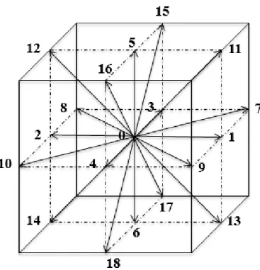
Figure 2.1. D3Q19 lattice model ... 11

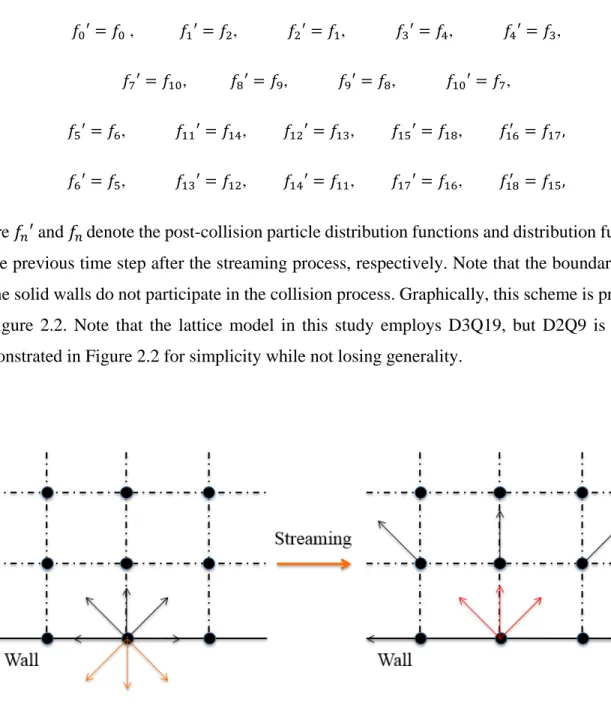
Figure 2.2. Half-way bounce-back boundary condition ... 12

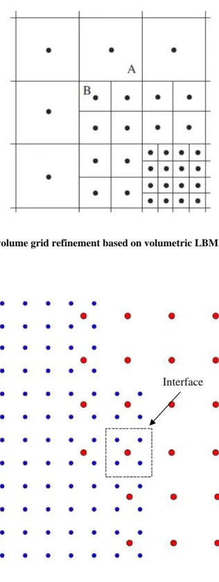
Figure 2.3. Finite-volume grid refinement based on volumetric LBM (Rohde et al. 2006) ... 18

Figure 2.4. Staggered grid arrangement for local grid refinement (Premnath et al. 2013a) ... 18

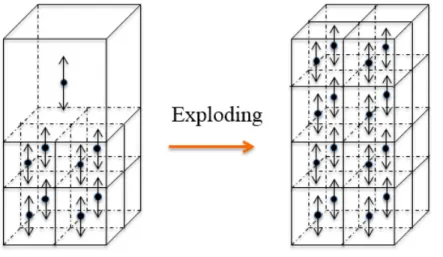
Figure 2.5. Graphical illustration of explode ... 20

Figure 2.6. Graphical illustration of coalesce ... 21

Figure 2.7. Wall-bounded channel (X: streamwise direction; Y: spanwise direction; Z: wall-normal direction) ... 23

Figure 2.8. Velocity profile for laminar channel flow ... 23

Figure 3.1. (a) Velocity profiles normalized using viscous length scale; (b) Velocity profiles normalized using half-channel height ... 27

Figure 3.2. (a) The streamwise normal Reynolds stress; (b) The Reynolds shear stress ... 29

Figure 3.3. Streamwise velocity at X-Y plane (z+ = 8.5) ... 30

Figure 3.4. Instantaneous X vorticity in transverse plane ... 31

Figure 3.5. Isosurface of vortex structures near the walls (Q = 1.5E-6) ... 31

Figure 4.1. Computational domain ... 35

Figure 4.2. Isosurface of vortex structures in precursor turbulent inflow (Q = 1.25) ... 36

Figure 4.3. Schematic of specification of inflow using precursor channel flow. ... 36

Figure 4.4. (a) Streamline and vectors of mean velocity in an enlarged X-Y plane (z/H = 0.5); (b) Streamline and vectors of mean velocity in an enlarged X-Z plane ... 38

Figure 4.5. Instantaneous vorticity in mid-height plane and vertical mid-plane ... 40

Figure 4.6. Instantaneous normalized SGS viscosity (𝝂𝝂SGS/𝝂𝝂0 = 0.35) ... 40

Figure 4.7. Visualization of instantaneous vortex structures using Q criterion (Q = 28) ... 41

Figure 4.8. (a) Instantaneous vortex structures in the gap region; (b) Instantaneous X vorticity in transverse plane. ... 41

(12)

xi

Figure 4.10. Mean flow structures of the gap region (Q = 1.80E-6) ... 44 Figure 4.11. Vortex structures visualized using Q criteria: (a) 1st_{eigenfunction (Q = 4.50E-7); (b)}

5th_{eigenfunction (Q = 4.50E-7); (c) 10}th_{eigenfunction (Q = 8.50E-7); (d) 50}th

(13)

xii

NOMENCLATURE

English symbols

A coefficient of van Driest damping function

𝐴𝐴𝑘𝑘𝑘𝑘 kth eigenvector

𝐶𝐶𝑓𝑓 skin friction coefficient

𝑐𝑐𝑠𝑠 speed of sound in lattice Boltzmann method (m/s)

𝐶𝐶𝑠𝑠 constant for the standard Smagorinsky subgrid-scale model

𝐷𝐷 spatial dimension (mm)

𝑅𝑅⃗𝑘𝑘 discrete speed vectors

𝐹𝐹⃗ external force field

𝑓𝑓𝑘𝑘 particle distribution function

𝑓𝑓𝑘𝑘′ post-collision particle distribution function

𝑓𝑓𝑘𝑘𝑒𝑒𝑒𝑒 equilibrium distribution

𝐻𝐻 cubic prism height (mm)

𝐼𝐼 identity matrix

𝑖𝑖 streamwise position in the pre-cursor domain

𝐽𝐽⃗ three-dimensional momentum field (kg∙m/s)

𝑗𝑗 spanwise position in the pre-cursor domain

(14)

xiii

𝐿𝐿𝑥𝑥 streamwise length of the target domain (mm)

𝐿𝐿𝑦𝑦 spanwise length of the target domain (mm)

𝐿𝐿𝑧𝑧 wall-normal height of the target domain (mm)

𝑚𝑚 velocity moment 𝑚𝑚𝑒𝑒𝑒𝑒 _{equilibrium moment} 𝑀𝑀 transformation matrix 𝜧𝜧 number of snapshots 𝑛𝑛 refinement factor 𝑃𝑃 pressure (Pa)

𝑅𝑅𝑅𝑅𝐻𝐻 Reynolds number based on the cubic prism height

𝑅𝑅𝑅𝑅𝑚𝑚 Reynolds number based on the bulk velocity

𝑅𝑅𝑅𝑅𝜏𝜏 Reynolds number based on the friction velocity

𝑆𝑆̂ diagonal collision matrix

𝑆𝑆𝑔𝑔𝑔𝑔𝑔𝑔 gap distance between cubic prims (mm)

𝑆𝑆𝑘𝑘 relaxation rate

𝑆𝑆𝑠𝑠 source term

𝑆𝑆𝑘𝑘,𝑗𝑗 strain rate tensor (s-1)

𝑆𝑆𝑆𝑆 Strouhal number

𝛿𝛿𝑆𝑆 temporal step (s)

∆𝑆𝑆𝑐𝑐 coarse grid temporal step (s)

(15)

xiv

𝑆𝑆𝑡𝑡 trace of the matrix

𝑈𝑈��⃗ three-dimensional velocity field (m/s)

𝑈𝑈+ _{normalized streamwise velocity using viscous length scale}

𝑈𝑈𝑐𝑐𝑐𝑐 centerline velocity (m/s)

𝑈𝑈𝑚𝑚 bulk velocity (m/s)

𝑈𝑈𝑚𝑚𝑔𝑔𝑥𝑥 maximum streamwise velocity (m/s)

𝑢𝑢𝜏𝜏 friction velocity (m/s)

𝑢𝑢 streamwise velocity component (m/s)

𝑣𝑣 spanwise velocity component (m/s)

𝑤𝑤 wall-normal velocity component (m/s)

𝑢𝑢𝑘𝑘,𝑗𝑗 velocity gradient tensor (m/s)

𝑢𝑢′ streamwise fluctuation component (m/s)

𝑣𝑣′ spanwise fluctuation component (m/s)

𝑤𝑤′ wall-normal fluctuation component (m/s)

〈𝑢𝑢〉 streamwise mean velocity (m/s)

〈𝑣𝑣〉 spanwise mean velocity (m/s)

〈𝑤𝑤〉 wall-normal mean velocity (m/s)

〈𝑢𝑢′𝑢𝑢′〉+ _{normalized streamwise Reynolds stress using viscous length scale}

〈𝑢𝑢′𝑤𝑤′〉+ _{normalized Reynolds shear stress using viscous length scale}

𝑋𝑋 coordinate in streamwise direction of the target domain

(16)

xv

𝛿𝛿𝑥𝑥 spatial step (mm)

∆𝑥𝑥 reference length scale (mm)

∆𝑥𝑥𝑐𝑐 coarse grid spacing (mm)

∆𝑥𝑥𝑓𝑓 fine grid spacing (mm)

∆𝑥𝑥+ _{normalized streamwise grid spacing using viscous length scale}

𝑌𝑌 coordinate in spanwise direction of the target domain

𝑦𝑦 spanwise position in the target domain (mm)

∆𝑦𝑦+ _{normalized spanwise grid spacing using viscous length scale}

𝑍𝑍 coordinate in wall-normal direction of the target domain

𝑧𝑧 wall-normal position in the target domain (mm)

𝑧𝑧+ _{normalized wall-normal distance using viscous length scale}

∆𝑧𝑧+ _{normalized wall-normal grid spacing using viscous length scale}

Greek symbols

𝜖𝜖 empirical constant

𝜆𝜆𝑘𝑘 kth eigenvalue

𝜈𝜈𝑐𝑐 coarse grid viscosity (m2/s)

𝜈𝜈𝑓𝑓 fine grid viscosity (m2/s)

𝜈𝜈0 molecular viscosity (m2/s)

𝜈𝜈𝑆𝑆𝑆𝑆𝑆𝑆 subgrid-scale viscosity (m2/s)

(17)

xvi

𝜏𝜏𝑤𝑤 wall shear stress (N/m2)

𝛷𝛷𝑘𝑘 kth eigenfunction

𝜔𝜔𝑘𝑘 weighing factor

(18)

1

CHAPTER 1 INTRODUCTION

1.1 Motivation

Turbulent flow is characterized by its irregular and chaotic instantaneous patterns. The research of such flows is inherently complex and challenging, yet also relevant to many industrial and environmental applications. Computational fluid dynamics (CFD) is a powerful technique that analyzes a fluid flow and the associated phenomena by means of numerical simulation. It finds wide applications in industrial research and design, including fluid dynamics of aircraft, turbomachinery, chemical processing and meteorology (Versteeg and Malalasekra 2007).

Experimental approaches and computational simulations are two effective tools for studying turbulence. As compared with experimental fluid dynamics, CFD demonstrates several unique advantages including a reduction of effort in building the experimental environment, the capability to study large-scale systems, and the availability of data and flow information everywhere in the computational domain.

Traditionally, the governing equations in CFD are the Navier-Stokes equations. These 2nd order nonlinear equations fundamentally determine macroscopic properties of the velocity and pressure fields in a fluid flow. The Navier-Stokes equations are nonlinear in nature and thus formidable to solve directly. Therefore, both computational techniques and theoretical models are required in solving these equations.

A novel numerical approach called the lattice Boltzmann method (LBM) has evolved over the past decades. Instead of solving the traditional Navier-Stokes equations, LBM seeks to perform the simulation through an algorithm that includes a collision model and a streaming process. This method demonstrates a relatively simple algorithm and is widely considered to be a potential alternative to the traditional methods adopted in CFD.

(19)

2

1.2 Literature review

The Lattice Boltzmann method (LBM) is a comparatively new and numerically efficient approach in computational fluid dynamics. It demonstrates the potential to become a promising alternative to the traditional Navier-Stokes equations and thus has found multiple applications in simulation of fluid flows (Yu 2004, Chikatamarla et al. 2010, Koda 2013, Hossain et al. 2015). The LBM is originally derived from the continuous Boltzmann equation through discretization in time and space, which describes a fluid system statistically based on the particle density distribution functions (He and Luo 1997). In fact, the Navier-Stokes equations for viscous flow can be recovered by applying the second-order Chapman-Enskog expansion to the continuous Boltzmann equation (Bespalko 2006). The LBM has also been mathematically characterized as a finite-difference-based scheme (He and Luo 1997, Yu 2004).

The flow field of the LBM consists of a number of fictitious particles moving along specified lattice directions at fixed velocities (Bespalko 2006). These particles collide and stream in a physical space that is discretized by a uniform grid. The macroscopic state at each lattice site can then be calculated from the corresponding particle distribution functions. Hence, implementation of the LBM involves two steps: collision and streaming. The collision process deals with their relaxation process to their local equilibrium, and the streaming process describes the movement of the particles along the specified directions to their neighbouring sites after the collision step (Premnath et al. 2009b). The LBM therefore demonstrates two key advantages over the traditional method: a simple algorithm and parallel scalability (Koda 2013). The former originates from the fact that there is no pressure solver involved in the algorithm to correct the velocity field; the pressure in the LBM is obtained from the local fluid density and the speed of sound.

Two collision models are widely used in the LBM: the single-relaxation-time (SRT) model and multiple-relaxation-time (MRT) model. The SRT is also referred to as the Bhatnager-Gross-Krook (BGK) model and has gained wide popularity for its simplicity in implementation (D'Humieres et al. 2002, Yu 2004). In the SRT-LBM, a single relaxation parameter essentially determines the rate at which the particle distributions relax to their local equilibrium, whereas the MRT model computes different relaxation rates in moment space (Premnath et al. 2009b). The

(20)

3

MRT LBM, also known as the generalized lattice Boltzmann method (GLBM), is generally preferred over the SRT LBM since it provides a higher numerical stability. This is especially the case for flows at high Reynolds numbers (Premnath et al. 2009b, Freitas et al. 2011). Additionally, optimal stability can be achieved by tuning the different relaxation rates individually (D'Humieres et al. 2002). The type of lattice models also has an impact on the capability of LBM. Several lattice models are particularly popular and widely employed for three-dimensional fluid flow simulation, including the three-dimensional, fifteen-particle velocity (D3Q15) lattice model, and models which are similarly described as D3Q19 and D3Q27. The number of velocity sites is one influencing factor to the numerical accuracy. However, a higher number of velocity sites typically also increases the computational load.

One major constraint imposed by the LBM in application to complex flows lies in its inherent uniformity in the computational domain. In order for the LBM to be effective in the exploration of complex fluid flows, this restriction should be circumvented. One effective approach to achieve this goal is local grid refinement. Over the past decades, a number of pioneering schemes have been proposed for local grid refinement. One early scheme proposed by He et al. (1996) is the interpolation-supplemented LBM. A continuously varying grid mesh is realized in this scheme where the values on the refined grid are simply obtained by interpolation from the coarse grid after each round of streaming and colliding. Filippova and Hanel (1998) proposed a popular scheme using the locally embedded grid. The entire computation domain is initially covered with the coarse grid. The fine grid is then patched to regions where turbulent eddy motions exist at small scales. Spatial and temporal interpolations are both implemented in this scheme to realize the communication between the coarse and the fine grids. Dupuis and Chopard (2003) developed a similar scheme to the one of Filippova and Hanel (1998), but using a simpler algorithm in interpolations with second-order accuracy. One common feature of the aforementioned schemes is that they are node-based, or finite-difference formulated, and interpolation of the surrounding nodes or rescaling serves as a critical step in implementing such local grid refinement. This approach does not inherently conserve mass, momentum and energy (Chen et al. 2006). One recent attempt to address this issue is the so-called imbalance correction grid refinement method proposed by Kuwata and Suga (2016). This approach is an extension to the work of Dupuis and Chopard (2003); a correction step is introduced to remove the unphysical discontinuity in the interface region serving to mitigate the non-conservation issue. Freitas et al.

(21)

4

(2006) developed a so-called hierarchical grid refinement. This refinement technique is also similar to the work of Filippova and Hanel (1998). However, one fundamental difference between them is that Freitas et al. (2006) used the cell-centered approach in their study and this makes it as a finite-volume-formulated scheme. In realizng this scheme, a non-linear interpoation is required along with a transformation of the non-equilibrium part of the distribution functions. Eitel-Amor et al. (2013) worked further on this scheme and developed a dynamic version of such local grid refinement called the hierarchical adaptive grid refinement. Instead of locating the refinement region manually, hierarchical adaptive grid refinement incorporates monitoring parameters in the scheme to determine the need of refinement for a region dynamically. In the study by Eitel-Amor et al. (2013), two dynamic parameters are used based on the absolute value of the vorticity vectors and the difference of the total pressure at low Mach numbers.

On the other hand, Chen et al. (2006) and Rohde et al. (2006) proposed a novel volumetrically formulated scheme. No interpolation is required to realize this local grid refinement while the laws of conservation are precisely satisfied in the grid transition. This scheme removes the extra steps in the algorithm associated with interpolation or rescaling. In addition, it removes the fact that the computational accuracy is directly related to the accuracy of the interpolation. The reduction in overall computational cost in this scheme is achieved by a factor of 16 for a coarse cubic grid (Premnath et al. 2013a). Fundamental explorations using classical turbulent channel flow based on this technique have demonstrated satisfactory results (Premnath et al. 2009(a, b)). Applications in complex flows using this technique (Premnath et al. 2013 (a, b) , Staubach 2013) have also yielded promising results. However, unphysical discontinuities are reported in some high-order statistics profiles (Rohde et al. 2006, Premnath et al. 2013a, Kuwata and Suga 2016). Athough the current limitation of the use of a uniform grid in the LBM has begun to be addressed over the previous decade, local grid refinement has not yet become a mature methodology. Therefore, additional studies are required to test and improve their predictive performance while ensuring the conservation laws are satisfied.

Large eddy simulation (LES) is a prevailing turbulence model that identifies two different eddy scales of turbulent flows through filtering: resolved-scale eddies with a length scale larger than the grid size and unresolved-scale eddies that are smaller than the grid size. LES computes the larger resolved-scale eddy motions by directly solving the governing equations without any ad

(22)

5

hoc assumption, and models the physical effects of the smaller unresolved-scale motions by using a subgrid-scale (SGS) model (Hou et al. 1996, Yu 2004). One such model is the standard Smagorinsky SGS model.This model has gained wide popularity over the past decades due to the fact that the turbulent eddy viscosity is based on a simple formulation using a strain-rate tensor. Incorporation of this traditional SGS model into the LBM was proposed early and demonstrated to be straightforward in implementation by Hou et al. (1996). It should be noted that significant differences exist in implementing LES based on the different governing equations. For the Navier-Stokes equations, the estimated eddy viscosity contributes to the evolution of the flow fields directly during the next time step, whereas for the LBM the eddy viscosity only alters the corresponding relaxation rates for the particle distribution functions which serve to specify the flow states (Yu 2004). Applications of LBM LES have been successfully implemented in many realistic flows (Yu 2004, Premnath et al. 2009a, Koda 2013, Hossain et al. 2015). However, such LBM LES has not yet been widely applied to the flow in wake regions where complex flow structures are expected.

1.3 Objectives

The present thesis will investigate the performance of LBM LES for studying turbulent near-wall flows. The research will begin with an in-house LBM code initially developed for micro-fluidic flows and later applied to simulation of a turbulent lid-driven cavity flow by Dr. Md. Shakhawath Hossain (Hossain et al. 2015). Three objectives are identified for the current research: 1. The first objective is to modify the in-house code to be able to predict turbulent wall-bounded channel flow. More specifically, it will be used to perform a Direct Numerical Simulation (DNS) of a turbulent channel flow for a low Reynolds number. The numerical results will be analyzed and compared to those of a well-documented study from the literature. Typical flow structures will also be studied.

2. A major limitation in applying the LBM to complex flows originates from the inherent uniformity of the grid over the computational domain. Therefore, the second objective of the current study is to improve the effectiveness of the LBM by implementing local grid

(23)

6

refinement. A laminar channel flow will be used for this investigation where the regions near the walls will be refined. The preliminary performance will be assessed by comparing the velocity profile to that of an analytical solution.

3. The third objective of the current research is to explore the capability of LBM LES in predicting the flow structures in a more complex flow than a typical channel flow. Geometric complexity will be increased by adding two cubic prisms on the bottom wall of the channel. A standard Smagorinsky SGS model will be incorporated in the framework of the LBM to realize an LES for this study. A pre-cursor inflow and a constant pressure are both required for the inlet and outlet boundary conditions, respectively. The three-dimensional coherent structures will also be analyzed using both of the second invariant criterion (Hunt et al. 1988) and a Proper Orthogonal Decomposition (Kim et al. 2005).

The scope of the current thesis will largely focus on the numerical methodology and its application to the turbulent channel flow and flow over wall-mounted cubes. A local grid refinement method will be introduced as an attempt to improve the potential application of the LBM to wall-bounded flows. However, due to the time constraint, the application will only be limited to a laminar channel flow. An LES based on a standard SGS model will be considered in this study. It will significantly enhance an in-house LBM code for performing LES of near-wall turbulent flows; however, it cannot address every feature of the LBM that could be potentially improved.

1.4 Thesis structure

The present thesis is organized as follows. The lattice Boltzmann method is introduced in Chapter 2 where the collision operator and lattice model employed in the current study are both described in detail. Chapter 2 also documents the boundary conditions, initial conditions, and the iterative algorithm for implementing the LBM code. A demonstration of volumetric grid refinement and its performance in a laminar channel flow is included in Chapter 2 as well.

(24)

7

Chapter 3 presents the LBM DNS of a turbulent channel flow where the performance of the developed code is validated by comparison to other results. The second invariant criterion is introduced in the same chapter to visualize the vortex structures.

The thesis then proceeds to demonstrate a LBM LES of the complex wake flow over two cubic prisms in Chapter 4. A standard Smagorinsky model is introduced as the SGS model. Both mean flow patterns and instantaneous flow structures are analyzed. A snapshot version of the POD (Kim et al. 2005) is also included to analyze the flow structures from a different perspective.

Finally, Chapter 5 identifies the conclusions drawn from the current research and provides views into the future work.

(25)

8

CHAPTER 2 LATTICE BOLTZMANN METHOD

2.1 Background

The current research essentially employs a MRT collision model to study three-dimensional turbulent flows based on a D3Q19 lattice model. This chapter aims to provide a detailed description of the numerical methodology and thereby is organized as follows. The MRT LBM and D3Q19 lattice model are presented in Section 2.2 and Section 2.3. The chapter then proceeds by describing the different boundary conditions, initial conditions and external forcing terms employed in the current study, in Sections 2.4 and 2.5. The implementation algorithm for the newly developed LBM code is discussed in Section 2.6. Finally, a detailed description of the selected local grid refinement method is given in Section 2.7, along with a preliminary performance test using a laminar channel flow.

2.2 Multiple Relaxation Time LBM

The evolution equation for the MRT LBM is given by (Yu 2004):

𝑓𝑓(𝑥𝑥⃗+𝑅𝑅⃗𝛿𝛿𝑆𝑆,𝑆𝑆+𝛿𝛿𝑆𝑆)− 𝑓𝑓(𝑥𝑥⃗,𝑆𝑆) =−𝑀𝑀−1_×_𝑆𝑆̂_{× [}_{𝑚𝑚 − 𝑚𝑚}𝑒𝑒𝑒𝑒_{], (2.1)} where𝑓𝑓(𝑥𝑥⃗,𝑆𝑆) represents the particle distribution function, and 𝑓𝑓(𝑥𝑥⃗+𝑅𝑅⃗𝛿𝛿𝑆𝑆,𝑆𝑆+𝛿𝛿𝑆𝑆) is a particle distribution function that describes the corresponding particle movement for the next time step,𝛿𝛿𝑆𝑆, to the neighbouring lattice node,𝛿𝛿𝑥𝑥, along a specified direction,𝑅𝑅⃗. Equation (2.1) is written using the convention that the LHS of the equation denotes the streaming process whereas the RHS signifies the cumulative effect of the collision process. 𝑆𝑆̂ stands for the diagonal collision matrix that determines the relaxation rates and is given by:

𝑆𝑆̂=𝑑𝑑𝑖𝑖𝑑𝑑𝑑𝑑 (𝑆𝑆1,𝑆𝑆2,𝑆𝑆3,𝑆𝑆4,𝑆𝑆5,𝑆𝑆6,𝑆𝑆7,𝑆𝑆8,𝑆𝑆9,𝑆𝑆10,𝑆𝑆11,𝑆𝑆12,𝑆𝑆13,𝑆𝑆14,𝑆𝑆15,𝑆𝑆16,𝑆𝑆17,𝑆𝑆18,𝑆𝑆19). (2.2) The detailed values of the above diagonal matrix are provided in Appendix .

(26)

9

In equation (2.1), 𝑀𝑀is a 19 × 19 matrix that linearly transforms the distribution functions into velocity moments (Yu 2004):

𝑚𝑚(𝑥𝑥,𝑆𝑆) =𝑀𝑀×𝑓𝑓(𝑥𝑥,𝑆𝑆), and 𝑓𝑓(𝑥𝑥,𝑆𝑆) =𝑀𝑀−1_×_𝑚𝑚₍_𝑥𝑥_,_𝑆𝑆_{), (2.3)} where the elements of 𝑀𝑀 and 𝑀𝑀−1are given in Appendix . The equilibrium moments in equation (2.1),𝑚𝑚𝑒𝑒𝑒𝑒, are functions of density and local velocities, details of which are specified in Appendix as well.

The fluid density and momentum in LBM are given by

𝜌𝜌=� 𝑓𝑓𝑘𝑘 18 𝑘𝑘=0 , and 𝜌𝜌𝑈𝑈��⃗ =� 𝑅𝑅��⃗𝑓𝑓𝚤𝚤 𝑘𝑘 18 𝑘𝑘=0 . (2.4𝑑𝑑,𝑏𝑏)

The sound speedis 𝑐𝑐_𝑠𝑠 =𝑐𝑐/√3, and 𝑐𝑐 = 𝛿𝛿𝑥𝑥/𝛿𝛿𝑆𝑆= 1 in lattice units. Physically, 𝛿𝛿𝑥𝑥 =

0.001 m 𝑑𝑑𝑛𝑛𝑑𝑑𝛿𝛿𝑆𝑆= 0.001 s, respectively. The molecular viscosity is given by

𝜈𝜈0 =₃𝑐𝑐�_𝑠𝑠1 𝑣𝑣−

1

2� 𝛿𝛿𝑥𝑥, (2.5)

where𝑠𝑠_𝑣𝑣 = 𝑠𝑠₁₀= 𝑠𝑠₁₂= 𝑠𝑠₁₄ = 𝑠𝑠₁₅= 𝑠𝑠₁₆ . In the current study, 𝑠𝑠_𝑣𝑣 = 1.98570 such that 𝜈𝜈₀ =

1.20 × 10−6_m2_/s.

The equilibrium distribution function for the LBM is given by

𝑓𝑓_𝑘𝑘𝑒𝑒𝑒𝑒= 𝜌𝜌𝜔𝜔𝑘𝑘�1 + 3�𝑅𝑅��⃗ ∙ 𝑈𝑈��⃗�𝚤𝚤 +₂9�𝑅𝑅��⃗ ∙ 𝑈𝑈��⃗�𝚤𝚤 2 −3₂𝑢𝑢2�,𝑖𝑖 = 0, 1,2, … ,18, (2.6) where ρ is the fluid density, 𝜔𝜔_𝑘𝑘 and 𝑅𝑅��⃗_𝚤𝚤are the weighting factors associated with the lattice model, and discrete velocity vectors, respectively. Both of them are specified in Section 2.3 below. In equation 2.6, 𝑈𝑈��⃗= 𝑈𝑈��⃗(𝑢𝑢(𝑥𝑥,𝑦𝑦,𝑧𝑧),𝑣𝑣(𝑥𝑥,𝑦𝑦,𝑧𝑧),𝑤𝑤(𝑥𝑥,𝑦𝑦,𝑧𝑧)) is the initial three-dimensional velocity field where u, v and w are velocity components at different locations in the domain.

(27)

10

2.3 D3Q19 lattice model

The D3Q19 lattice model has a total of nineteen discrete velocities. The corresponding discrete vectors are given by

𝑅𝑅𝚤𝚤 ��⃗= ⎩ ⎪ ⎨ ⎪ ⎧ (0, 0, 0), 𝑖𝑖= 0; (±1, 0, 0), (0, ±1, 0), (0, 0, ±1) 𝑖𝑖 = 1, 2, … ,6; (±1, ±1, 0), (±1, 0, ±1), (0, ±1, ±1) 𝑖𝑖 = 7, 8, … ,18.

The values of the weighting factors,𝜔𝜔_𝑘𝑘, are dependent on the lattice model. For the D3Q19 lattice model, they are specified as

𝜔𝜔𝑘𝑘 = ⎩ ⎪ ⎪ ⎨ ⎪ ⎪ ⎧ 1_{3 ,} 𝑖𝑖= 0; 1 18 , 𝑖𝑖 = 1, 2, … ,6; 1 36 , 𝑖𝑖= 7, 8, … ,18.

(28)

11

Figure 2.1. D3Q19 lattice model

2.4 Boundary conditions

When the particles reach the boundaries of the computational domain after streaming and collision, information on the particle density distribution functions is not provided for the next time step. Boundary conditions, therefore, serve to provide the unknown information for the distribution functions, thus meeting the constraints imposed along the boundaries. Four types of LBM schemes are introduced in the current study to realize different boundary conditions. They are presented in detail in the following subsections.

2.4.1 Halfway bounce-back boundary condition

The halfway bounce-back scheme realizes the no-slip boundaries at solid walls. It represents second-order accuracy for plane walls and first-order accuracy for curved boundaries (He et al. 1997, Freitas et al. 2011). This scheme is named “halfway bounce-back” since the exact

(29)

12

no-slip location is implemented halfway between the fictitious boundary node and the first inner node by simply “bouncing back” the incoming particles to their opposite directions, i.e.

𝑓𝑓0′=𝑓𝑓0 , 𝑓𝑓1′=𝑓𝑓2, 𝑓𝑓2′=𝑓𝑓1, 𝑓𝑓3′=𝑓𝑓4, 𝑓𝑓4′=𝑓𝑓3, 𝑓𝑓7′=𝑓𝑓10, 𝑓𝑓8′=𝑓𝑓9, 𝑓𝑓9′=𝑓𝑓8, 𝑓𝑓10′=𝑓𝑓7,

𝑓𝑓5′=𝑓𝑓6, 𝑓𝑓11′=𝑓𝑓14, 𝑓𝑓12′=𝑓𝑓13, 𝑓𝑓15′=𝑓𝑓18, 𝑓𝑓16′ =𝑓𝑓17, 𝑓𝑓6′=𝑓𝑓5, 𝑓𝑓13′=𝑓𝑓12, 𝑓𝑓14′=𝑓𝑓11, 𝑓𝑓17′=𝑓𝑓16, 𝑓𝑓18′ =𝑓𝑓15,

where 𝑓𝑓_𝑛𝑛′ and 𝑓𝑓_𝑛𝑛denote the post-collision particle distribution functions and distribution functions of the previous time step after the streaming process, respectively. Note that the boundary nodes on the solid walls do not participate in the collision process. Graphically, this scheme is presented in Figure 2.2. Note that the lattice model in this study employs D3Q19, but D2Q9 is the one demonstrated in Figure 2.2 for simplicity while not losing generality.

(30)

13

2.4.2 Periodic boundary condition

A periodic boundary condition essentially connects the inlet and outlet in the specified direction such that the fluid flow in the domain follows a periodic pattern. This condition is simply realized by connecting the lattice nodes at the outlet to the corresponding lattice nodes at the inlet. Consequently, no single particle leaves the computational domain and the laws of conservation are well preserved. When a periodic boundary condition is applied, a sufficiently large domain should be used such that there is negligible statistical correlation between any two points separated by a distance equal to half of the computational domain (Rohde et al. 2006).

2.4.3 Precursor inlet boundary condition

A precursor inlet boundary condition provides an instantaneous inlet velocity profile for the downstream domain by extracting the velocity profile at each time step from an upstream periodic quasi-steady-state flow. This boundary condition is implemented by providing the distribution functions at the downstream inlet plane with velocity information at the upstream outlet, and density of the first inner nodes in the downstream domain, i.e. (Koda 2013)

𝑓𝑓𝑘𝑘 =𝑓𝑓𝑘𝑘eq�𝜌𝜌(𝑥𝑥+ 1,𝑦𝑦,𝑧𝑧),𝑈𝑈��⃗(𝑖𝑖,𝑗𝑗,𝑘𝑘)�, (2.7) where 𝑓𝑓_𝑘𝑘 and 𝑓𝑓_𝑘𝑘eq represent the particle distribution functions and equilibrium distribution functions at the inlet plane of the downstream domain, respectively. Here 𝜌𝜌(𝑥𝑥+ 1,𝑦𝑦,𝑧𝑧) denotes the density of the first inner nodes in the downstream domain, and 𝑈𝑈��⃗(𝑖𝑖,𝑗𝑗,𝑘𝑘) stands for the instantaneous velocities at the upstream outlet. A schematic diagram and details of the application are included in Section 4.3.

(31)

14

2.4.4 Constant pressure outlet boundary condition

The pressure at the outlet,𝑃𝑃_out, is maintained as constant via setting the density as constant,𝜌𝜌_out= constant, since in the LBM 𝜌𝜌_out= 𝑃𝑃_out/𝑐𝑐_𝑠𝑠2. Therefore, the particle distribution functions at the outlet need to be modified as follows (Mussa et al. 2009):

𝑓𝑓𝑘𝑘 = 𝑓𝑓𝑘𝑘𝑒𝑒𝑒𝑒�𝜌𝜌out(𝑥𝑥,𝑦𝑦,𝑧𝑧),𝑈𝑈��⃗(𝑥𝑥 −1,𝑦𝑦,𝑧𝑧)�, (2.8) where 𝑈𝑈��⃗(𝑥𝑥 −1,𝑦𝑦,𝑧𝑧) denotes the velocity field of the last inner nodes prior to the outlet plane of the target domain.

2.5 External force

The current LBM scheme incorporates a source term in the equations for the particle distribution functions to simulate the effect of a pressure gradient to drive the fluid flow. With the source term added, the evolution equation takes the form of (Premnath et al. 2009a)

𝑓𝑓(𝑥𝑥⃗+𝑅𝑅⃗𝛿𝛿𝑆𝑆,𝑆𝑆+𝛿𝛿𝑆𝑆)− 𝑓𝑓(𝑥𝑥⃗,𝑆𝑆) =−𝑀𝑀−1_×_𝑆𝑆̂_{× [}_{𝑚𝑚 − 𝑚𝑚}𝑒𝑒𝑒𝑒_{] +}_𝑀𝑀−1_×_{�𝐼𝐼 −}1

2𝑆𝑆̂�×𝑆𝑆𝑠𝑠, (2.9)

where the second term on the RHS of the above equation (2.9) introduces the effects of the pressure gradient. I is a 19×19 identity matrix and 𝑆𝑆_𝑠𝑠denotes the source term in moment space, the components of which are specified in Appendix.

A corresponding forcing term is also introduced in the relation for the local momentum field, i.e. 𝚥𝚥⃗=𝜌𝜌𝑈𝑈��⃗= � 𝑓𝑓𝑘𝑘𝑅𝑅��⃗𝚤𝚤+ 18 𝑘𝑘=0 1 2𝐹𝐹⃗𝛿𝛿𝑡𝑡, (2.10)

where 𝚥𝚥⃗=𝚥𝚥⃗�𝑗𝑗_𝑥𝑥,𝑗𝑗_𝑦𝑦,𝑗𝑗_𝑧𝑧� is the momentum field, 𝑈𝑈��⃗denotes the local velocity field and 𝐹𝐹⃗ =

(32)

15

equation (2.9) is essentially a function of the external force,��⃗𝐹𝐹, and local velocity, ��⃗𝑈𝑈. For the turbulent channel flow, the external force field is determined by (Jafari et al. 2014)

𝐹𝐹𝑥𝑥 = −𝑑𝑑𝑃𝑃_{𝑑𝑑𝑥𝑥} = 8_𝐿𝐿𝜏𝜏𝑤𝑤 𝑧𝑧 =

8𝜌𝜌𝑢𝑢𝜏𝜏2

𝐿𝐿𝑧𝑧 ,𝐹𝐹𝑦𝑦 = 0,𝐹𝐹𝑧𝑧 = 0, (2.11) In equation 2.11, 𝑑𝑑𝑃𝑃/𝑑𝑑𝑥𝑥 is the pressure gradient, 𝜏𝜏_𝑤𝑤is the wall shear stress, 𝐿𝐿_𝑧𝑧denotes the channel height, and 𝑢𝑢_𝜏𝜏is the friction velocity.

2.6 Initial condition

A sinusoidal perturbation, superimposed on a one-seventh power law for the mean velocity profile in all three dimensions, serves as the initial condition for the fluid flow in the current study. These perturbations attempt to trigger turbulence in the early stage of development. Note that the initial condition does not affect the quasi-steady state; the initial state only serves to reduce the computational effort it takes to reach the fully developed state. Mathematically, the perturbations are expressed as (Lam 1989)

𝑢𝑢′₌ _{𝜖𝜖𝐿𝐿} 𝑥𝑥sin�𝜋𝜋𝑧𝑧_𝐿𝐿 𝑧𝑧� �cos 2𝜋𝜋𝑥𝑥 𝐿𝐿𝑥𝑥 sin 2𝜋𝜋𝑦𝑦 𝐿𝐿𝑦𝑦 + 1 2 cos 4𝜋𝜋𝑥𝑥 𝐿𝐿𝑥𝑥 sin 2𝜋𝜋𝑦𝑦 𝐿𝐿𝑦𝑦 + cos 2𝜋𝜋𝑥𝑥 𝐿𝐿𝑥𝑥 sin 4𝜋𝜋𝑦𝑦 𝐿𝐿𝑦𝑦 �, (2.12) 𝑣𝑣′₌ _{−𝜖𝜖𝐿𝐿} 𝑦𝑦sin�𝜋𝜋𝑧𝑧_𝐿𝐿 𝑧𝑧� � 1 2 sin 2𝜋𝜋𝑥𝑥 𝐿𝐿𝑥𝑥 cos 2𝜋𝜋𝑦𝑦 𝐿𝐿𝑦𝑦 + 1 2 sin 4𝜋𝜋𝑥𝑥 𝐿𝐿𝑥𝑥 cos 2𝜋𝜋𝑦𝑦 𝐿𝐿𝑦𝑦 + 1 4 sin 2𝜋𝜋𝑥𝑥 𝐿𝐿𝑥𝑥 cos 4𝜋𝜋𝑦𝑦 𝐿𝐿𝑦𝑦 �, (2.13) 𝑤𝑤′₌ _{−𝜖𝜖 �}_{1 + cos}𝜋𝜋𝑧𝑧 𝐿𝐿𝑧𝑧� �sin 2𝜋𝜋𝑥𝑥 𝐿𝐿𝑥𝑥 sin 2𝜋𝜋𝑦𝑦 𝐿𝐿𝑦𝑦 + sin 4𝜋𝜋𝑥𝑥 𝐿𝐿𝑥𝑥 sin 2𝜋𝜋𝑦𝑦 𝐿𝐿𝑦𝑦 + sin 2𝜋𝜋𝑥𝑥 𝐿𝐿𝑥𝑥 sin 4𝜋𝜋𝑦𝑦 𝐿𝐿𝑦𝑦 �, (2.14) where 𝑢𝑢′,𝑣𝑣′and 𝑤𝑤′represent the sinusoidal fluctuations in the streamwise (X), spanwise (Y) and wall-normal (Z) directions, respectively. Note that x, y, and z signify the corresponding locations in the X, Y, and Z directions.𝐿𝐿_𝑥𝑥,𝐿𝐿_𝑦𝑦 and 𝐿𝐿_𝑧𝑧denote the total length of the computational domain in the X, Y and Z directions. 𝜖𝜖 is an empirical constant determining the magnitude of the perturbations

(33)

16

and, in the current study, is set to 𝜖𝜖 = 3.65 × 10-5. Note that an inappropriate 𝜖𝜖value may result in divergence or delaying triggering of turbulence.

Consequently, the three components of the velocity field in the equilibrium distribution functions (Eqn. 2.6) become

𝑢𝑢 =〈𝑢𝑢〉+𝑢𝑢′_,_𝑣𝑣₌ _{〈𝑣𝑣〉}₊_𝑣𝑣′_,_𝑤𝑤 ₌ _{〈𝑤𝑤〉}₊_𝑤𝑤′_,

where, for turbulent channel flow, 〈𝑢𝑢〉 is the streamwise velocity determined using the one-seventh power law, and 〈𝑣𝑣〉=〈𝑤𝑤〉= 0.

2.7 Implementation of the LBM code

The iterative steps for implementing the basic LBM algorithm are as follows:

1) Initial conditions

This step defines the relevant parameters and variables, specifies the computational domain, and determines the macroscopic properties, etc.

2) Equilibrium distribution functions

This step specifies the initial state of the fluid flow. The initial conditions of the fluid velocity field and the perturbations are implemented in this step.

3) Collision process

The external force that simulates the pressure gradient driving the flow is implemented in this step. Note that the wall nodes where no-slip boundary conditions are applied do not participate in this step.

4) Boundary conditions

5) Streaming step

(34)

17

Back to step 3) until quasi-steady state developed.

6) Post-processing subroutines

Subroutines in this step process the data sets for analysis and visualization after reaching the quasi-steady state.

2.8 Local grid refinement

This subsection studies the volumetric local grid refinement proposed by Chen et al. (2006) and Rohde et al. (2006). This approach is preferred over other schemes because it is a finite-volume-based scheme and presents promising results while involving a comparatively simple algorithm. A locally refined laminar channel flow is simulated in this subsection to test the basic performance of this refinement scheme. The results will be compared to the analytical solution.

2.8.1 Volumetric grid refinement

Implementation of volumetrically formulated grid refinement relies on the volumetric description of the LBM. This concept is illustrated in Figure 2.3. Rather than the original particle distribution function on each lattice node, it is the mass distribution function on each cell that is now under consideration. Within each single cell volume, particle densities are assumed to be uniform everywhere. This re-interpretation of LBM results in a staggered grid arrangement schematically shown in Figure 2.4. One character of volumetric grid refinement that distinguishes itself from the other schemes is that the fine grid cell (Cell B in Figure 2.3) and the coarse grid cell (Cell A in Figure 2.3) do not share the identical spatial or temporal scales. These scales are proportionally associated with the grid refinement factor, n, such that spatially ∆𝑥𝑥_𝑐𝑐 =

𝑛𝑛∆𝑥𝑥𝑓𝑓 and temporally ∆𝑆𝑆𝑐𝑐 =𝑛𝑛∆𝑆𝑆𝑓𝑓 where f and c denote the fine grid and coarse grid, respectively (Rohde et al. 2006).

(35)

18

Figure 2.3 Finite-volume grid refinement based on volumetric LBM (Rohde et al. 2006)

Figure 2.4. Staggered grid arrangement for local grid refinement (Premnath et al. 2013a) Interface

(36)

19

During the computation, the fine grid covers the regions where turbulent structures at small scales exist, i.e. near-wall regions and regions in proximity to surface geometry. The rest of the domain is taken care of by the coarse grid where fairly large structures are expected. There exists a single interface layer shown in Figure 2.4 where both grids overlap, serving the role of communication between the two grids. Two critical steps are implemented for this interconnection: explode and coalesce. The former deals with the transition from the coarse grid to the fine grid, and the latter works the other way around. In the explode step, the information on the post-collision state for the coarse grid in the interface is uniformly redistributed to the fine grid. Conversely, in the coalesce step, the pre-collision state fine grid in the interface layer provides the input for the corresponding coarse grid (Chen et al. 2006). Note that these two steps, explode and coalesce, are implemented only on the directions pointing into the fine grid and the coarse grid, respectively (Rohde et al. 2006).

2.8.2 Algorithmic steps

The detailed algorithmic steps implemented for local grid refinement are specified below following Chen et al. (2006) and Rohde et al. (2006):

1) Explode

Over the interface, mass distribution in a coarse grid cell is uniformly redistributed into a number of 𝑛𝑛𝐷𝐷fine grid cells, with 𝑛𝑛 denoting the refinement factor and 𝐷𝐷the spatial dimension. Normally 𝑛𝑛 is an even number and in this case, 𝑛𝑛= 2 and𝐷𝐷 = 3. This process is graphically illustrated in Figure 2.5. Note that the densities do not change and are assumed to be uniform anywhere. No interpolation or rescaling is required here.

(37)

20

Figure 2.5. Graphical illustration of explode

2) Standard streaming step on the fine nodes

3) Standard collision step on the fine nodes

The collision step is performed on the fine nodes for this step along with the external force, if there is any. Note that this step is not performed on the fine nodes located in the overlap region.

4) Application of wall boundary conditions on the current grid level

5) Repeat steps 2) to 4) n-1 times

It should be reiterated that the fine grid and the coarse grid do not share the identical spatial or temporal scales; these scales are related to n such that∆𝑥𝑥_𝑐𝑐 =𝑛𝑛∆𝑥𝑥_𝑓𝑓 and ∆𝑆𝑆_𝑐𝑐 =

𝑛𝑛∆𝑆𝑆𝑓𝑓. Therefore, in this case, the fine grid takes two time steps for each time step taken by the coarse grid in each iteration.

6) Standard streaming step on the coarse nodes

7) Coalesce

This step is the converse of the explode step; summation of the mass distribution on the fine cells to provide information for the corresponding coarse cell over the interface region.

(38)

21

Again, note that neither interpolation nor rescaling is performed in this step. Graphically, this step is shown in Figure 2.6 below

Figure 2.6. Graphical illustration of coalesce

8) Standard collision step on the coarse nodes 9) Back to step 1)

2.8.3 Performance of local grid refinement

Exploration of the volumetric local grid refinement started with a numerical validation using a fully developed laminar channel flow. A creeping laminar flow in the wall-bounded channel with a Reynolds number of 𝑅𝑅𝑅𝑅 =𝑈𝑈_{𝑐𝑐𝑐𝑐}(𝐿𝐿_𝑧𝑧/2)/𝜈𝜈₀ ≈1.08 was considered; 𝑈𝑈_{𝑐𝑐𝑐𝑐},𝐿𝐿_𝑧𝑧 and 𝜐𝜐₀ here denote the centerline velocity, channel height and molecular viscosity, respectively. No-slip boundary conditions were applied to the top and bottom walls using the halfway bounce-back scheme. Periodic boundary condition was realized in the streamwise and spanwise directions, respectively. An external force simulating the effect of pressure gradient was used to drive the flow. Details are provided in Section 2.5 in terms of modifying the particle distribution functions to incorporate the external force field.

(39)

22

Two grid resolutions, i.e.𝑛𝑛 = 2, were implemented in the computational domain where the coarse grid was applied in the center, and regions near the walls were refined using the fine grid. The height of each of the fine grid layers is 14 fine unit cells, which is 7 coarse unit cells. Meanwhile, since 𝜈𝜈₀ = (1/3)((1/𝑠𝑠_𝑣𝑣)−(1/2))𝑐𝑐𝛿𝛿𝑥𝑥 for the coarse grid, the corresponding relaxation parameters related to the molecular viscosity on the fine grid were adjusted such that the viscosities match on both grids, i.e. 𝜈𝜈_𝑐𝑐 = (1/𝑛𝑛)𝜈𝜈_𝑓𝑓. The corresponding numerical specifications are summarized in Table 2.1 and the computational domain is illustrated in Figure 2.7.

A plot of the predicted velocity profile is presented in Figure 2.8. The laminar velocity profile agrees very well with its analytical solution. Slight discrepancies are observed at two locations: under-estimation in proximity to the wall and over-estimation in the overlap region. The former originates from the halfway bounce-back scheme, and the latter could be due to the transfer of the numerical information. This over-estimation is quantified as 2.89% in this case by comparison with the analytical solution. A non-physical discontinuity is not observed here.

The current simulation of laminar channel flow only serves as a preliminary test of the performance of the local grid refinement method. Further testing is required and could be performed using turbulent channel flow. Note that in turbulent channel flow, the grid resolution used here is not sufficiently fine to capture the turbulence perfectly well. But lower-order turbulence statistics profiles are expected to match well with the documented results.

Table 2.1. Specifications of computational domain

Coarse grid Fine grid

Computational domain𝑳𝑳_𝒙𝒙×𝑳𝑳_𝒚𝒚×𝑳𝑳_𝒛𝒛: 128 × 64 × 64 256 × 128 × 128

Coarse grid size 128 × 64 × 50

-Fine grid size (top and bottom walls) - 256 × 128 × 14

Molecular viscosity (m2_/s) _{1.2 × 10}-6 _{2.4 × 10}-6

Density (kg/m3₎ _1.0 _1.0

(40)

23

Figure 2.7. Wall-bounded channel (X: streamwise direction; Y: spanwise direction; Z: wall-normal direction)

(41)

24

CHAPTER 3 LBM DNS OF TURBULENT CHANNEL FLOW

Turbulent channel flow is a typical benchmark case in fluid mechanics that has been studied extensively, partly because it provides understanding of the basic physics of wall-bounded turbulence and due to its geometric simplicity. The code developed in the current study will be validated by comparing the mean flow variables and lower-order statistics with those of a turbulent channel flow investigated by Kim et al. (1987) via DNS based on the Navier-Stokes equations.

Kim et al. (1987) studied this flow using a mesh size of 192 × 160 × 129 in the streamwise (X), spanwise (Y) and wall-normal (Z) directions, respectively. A Reynolds number of 𝑅𝑅𝑅𝑅_𝜏𝜏 =

𝑢𝑢𝜏𝜏(𝐿𝐿𝑧𝑧/2)/𝜈𝜈0 ≈180 was realized in their simulation, where 𝑢𝑢𝜏𝜏 is the friction velocity and 𝐿𝐿𝑧𝑧is the channel height. They applied periodic boundary conditions to the streamwise and spanwise directions, and the no-slip boundary conditions to the top and bottom walls, respectively. The grid spacing in the streamwise and spanwise directions was 𝛥𝛥𝑥𝑥+ ≈12, and 𝛥𝛥𝑦𝑦+ ≈ 7, respectively. A non-uniform mesh was employed in the wall-normal direction with the first inner node located at

𝑧𝑧+ _≈_0.05._{In the center of the channel,}_{𝛥𝛥𝑧𝑧}+ _≈_4.4._{The numerical study of Kim}_{et al.}_{(1987) has} been validated by comparison with experiments and has served as a benchmark for evaluating the quality of other numerical simulations of turbulent channel flow, though slight discrepancies were recognized in the comparisons of higher-order statistics profiles.

This chapter aims to validate the predictions of the LBM code for a turbulent channel flow from different perspectives and is organized as follows. The computational specifications of the current simulation will be introduced in Section 3.2, followed by the data comparison using the mean flow variables, the velocity profiles and Reynolds stress profiles in Section 3.3. Data visualizations will then be presented and discussed in Section 3.4.

(42)

25

3.2 Computational specifications

The current simulation was realized using a grid size of 396 × 105 × 198 in the X, Y and Z directions, respectively. The grid was uniformly configured in all three directions, and the spacing in wall units was𝛥𝛥+ ≈2.38. The first inner node in the wall-normal direction was located at

𝛥𝛥𝑧𝑧+ _≈_1.19._{Periodic boundary conditions were applied in the streamwise and spanwise} directions, and no-slip boundary conditions were realized at the top and bottom walls using a halfway bounce-back scheme. A Reynolds number of 𝑅𝑅𝑅𝑅_𝜏𝜏 = 𝑢𝑢_𝜏𝜏(𝐿𝐿_𝑧𝑧/2)/𝜈𝜈₀ ≈230 was achieved in the current simulation, slightly higher than that of Kim et al. (1987). Though this difference does yield a slightly stronger turbulence field, it is possible to make explicit comparisons using the normalized results. The fluid flow initially started with a predetermined mean velocity profile based on the one-seventh power law. Sinusoidal perturbations were superimposed in all three directions. The relevant details of the initial conditions are specified in Section 2.5. An external forcing term was employed to simulate the effects of a pressure gradient to drive the flow. It should be reiterated that the initial perturbations do not affect the fully-developed state of the fluid flow; they essentially serve to expedite the development of turbulence. The time-averaged quantities in the following sections are all based on the mean values calculated over 174,000 time steps after the flow had reached a quasi-steady state.

3.3 Mean flow properties

The mean flow variables of the current simulation are summarized in Table 3.1 along with those of the study by Kim et al. (1987). Given that the current DNS of turbulent channel flow represents a slightly higher Reynolds number, the mean flow variables of two studies agree well with one another. Meanwhile, the ratio of the centerline velocity to bulk velocity, 𝑈𝑈_{𝑐𝑐𝑐𝑐}/𝑈𝑈_𝑚𝑚, and the skin friction coefficient, 𝐶𝐶_𝑓𝑓, of the current study also match well with the correlations suggested by Dean (1978), i.e.

𝑈𝑈𝑐𝑐𝑐𝑐

𝑈𝑈𝑚𝑚 = 1.28𝑅𝑅𝑅𝑅𝑚𝑚

(43)

26

𝐶𝐶𝑓𝑓 = 0.073𝑅𝑅𝑅𝑅𝑚𝑚−0.25, (3.2) where 𝑅𝑅𝑅𝑅_𝑚𝑚 is the Reynolds number based on the bulk velocity and the entire channel height, 𝐿𝐿_𝑧𝑧. The bulk velocity is calculated based on the streamwise mean velocity,〈𝑢𝑢〉, i.e.

𝑈𝑈𝑚𝑚 =1₂� 〈𝑢𝑢〉 2 0 𝑑𝑑 �

𝑧𝑧

𝐿𝐿𝑧𝑧/2�. (3.3)

Table 3.1. Mean flow results for turbulent channel flow

Kim et al. (1987) Current study Dean (1978)

𝑅𝑅𝑅𝑅𝜏𝜏 = 𝑢𝑢𝜏𝜏(𝐿𝐿_{2 )}𝑧𝑧 𝜈𝜈0 180 230 - 𝑈𝑈𝑚𝑚 𝑢𝑢𝜏𝜏 15.63 16.76 - 𝑈𝑈𝑐𝑐𝑐𝑐 𝑢𝑢𝜏𝜏 18.20 19.83 - 𝑈𝑈𝑐𝑐𝑐𝑐 𝑈𝑈𝑚𝑚 1.16 1.18 1.15 𝐶𝐶𝑓𝑓 =₁ 𝜏𝜏𝑤𝑤 2𝜌𝜌𝑈𝑈𝑚𝑚2 8.18×10 -3 _7.12×10-3 _7.76×10-3

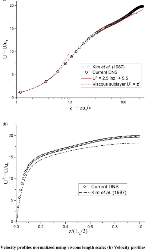
Figures 3.1(a) and 3.1(b) present the streamwise mean velocity profiles as a function of wall normal distance normalized by the viscous length scale and channel half-height, respectively. The mean velocity profile in wall units of the current DNS agrees well with both of the canonical logarithmic law and the profile of Kim et al. (1987). The current mean velocity plotted against the normalized coordinate (𝑧𝑧/(𝐿𝐿_𝑧𝑧/2)) sits higher than the profile of Kim et al. (1987). This difference largely originates from the higher Reynolds number in the current study.

(44)

27

Figure 3.1. (a) Velocity profiles normalized using viscous length scale; (b) Velocity profiles normalized using half-channel height

(a)

(45)

28

Two normalized Reynolds stress profiles, i.e. 〈𝑢𝑢′𝑢𝑢′〉+and〈𝑢𝑢′𝑤𝑤′〉+, are presented in Figures 3.2(a) and 3.2(b), respectively. These stresses represent the horizontal and vertical flux of streamwise turbulent momentum. Mathematically, based on the DNS data sets, these two terms are evaluated as follows:

〈𝑢𝑢′𝑢𝑢′〉+ ₌_〈𝑢𝑢′_𝑢𝑢′_〉_/_𝑢𝑢

𝜏𝜏2 = (〈𝑢𝑢𝑢𝑢〉 − 〈𝑢𝑢〉〈𝑢𝑢〉)/𝑢𝑢𝜏𝜏2, (3.4)

〈𝑢𝑢′𝑤𝑤′〉+ ₌_〈𝑢𝑢′_𝑤𝑤′_〉_/_𝑢𝑢

𝜏𝜏2 = (〈𝑢𝑢𝑤𝑤〉 − 〈𝑢𝑢〉〈𝑤𝑤〉)/𝑢𝑢𝜏𝜏2, (3.5) where 〈 〉 signifies time-averaging operation, 𝑢𝑢 =〈𝑢𝑢〉+𝑢𝑢′ and 𝑤𝑤= 〈𝑤𝑤〉+𝑤𝑤′. Both stress profiles are in reasonably good agreement with the reference values (at a lower Reynolds number). The slight over-predictions observed, especially in terms of the peak values, are believed to arise from the difference in Reynolds numbers. On the other hand, due to the comparatively coarse grid in proximity to the wall, the friction velocity was slightly inaccurate. This also contributes to the discrepancy in the Reynolds stress profiles. Based on the comparisons, the grid resolution employed was sufficient to predict the 2nd order statistics profiles reasonably well.

(a)

(46)

29

Figure 3.2. (a) The streamwise normal Reynolds stress; (b) The Reynolds shear stress

3.4 Near-wall structures

Elongated streaks of fluid with low streamwise velocity are observed in Figure 3.3 at an X-Y plane located at𝑧𝑧+ = 8.5. Figure 3.4 shows the instantaneous in-plane vorticity at four individual X-Z cross-sections. Strong vortices are identified in the near-wall regions as expected. Both the intensity and magnitude of the vorticity increases in the vicinity of the walls. Near the centerline, larger vortex structures are clearly identified.

Figure 3.5 visualizes the instantaneous vortex structures in the turbulent channel flow using the second invariant criterion. The second invariant criterion, or Q criterion, is a popular criterion for identifying a local fluid region as a vortex, i.e. vorticity is dominant when Q > 0 (Hunt et al. 1988). This concept could be illustrated using an expression by (Jeong and Hussain 1995):

𝑄𝑄 ≡1₂�𝑢𝑢𝑘𝑘2,𝑗𝑗 − 𝑢𝑢𝑘𝑘,𝑗𝑗𝑢𝑢𝑗𝑗,𝑘𝑘� =−1₂𝑢𝑢𝑘𝑘,𝑗𝑗𝑢𝑢𝑗𝑗,𝑘𝑘 =1₂��Ω𝑘𝑘,𝑗𝑗�2− �𝑆𝑆𝑘𝑘,𝑗𝑗�2�> 0, (3.6)

(b)

(47)

30

where 𝑢𝑢_𝑘𝑘_,_𝑗𝑗 represents the velocity gradient tensor, �Ω_𝑘𝑘_,_𝑗𝑗�2 = 𝑆𝑆𝑡𝑡�Ω_𝑘𝑘_,_𝑗𝑗Ω_𝑘𝑘_,_𝑗𝑗𝑡𝑡�and �𝑆𝑆_𝑘𝑘_,_𝑗𝑗�2 =

𝑆𝑆𝑡𝑡�𝑆𝑆𝑘𝑘,𝑗𝑗𝑆𝑆𝑘𝑘,𝑗𝑗𝑡𝑡� with 𝑆𝑆𝑡𝑡 signifying the trace of a matrix. Ω𝑘𝑘,𝑗𝑗 and 𝑆𝑆𝑘𝑘,𝑗𝑗 denote the local vorticity tensor and strain rate tensor, which mathematically are given by

Ω𝑘𝑘,𝑗𝑗 = 1₂�𝑢𝑢𝑘𝑘,𝑗𝑗− 𝑢𝑢𝑘𝑘,𝑗𝑗� and (3.7)

𝑆𝑆𝑘𝑘,𝑗𝑗 =1₂�𝑢𝑢𝑘𝑘,𝑗𝑗+𝑢𝑢𝑘𝑘,𝑗𝑗�. (3.8) In Figure 3.5, small-scale vortical structures are clearly captured in the near-wall regions. Many structures are similar to the classical hairpin structures. Generation of new hairpin structures, i.e. hairpin packets, are observed as well. These are expected typical flow features which are widely visualized and well documented in the literature pertaining to the turbulent boundary layer. However, complete prototypical hairpin structures are not very clear. This may be due to the low Reynolds number and comparatively coarse grid spacing in proximity to the wall.

Figure 3.3. Streamwise velocity at X-Y plane (z+_{= 8.5)}

Elongated streaks

X Y

(48)

31

Figure 3.4. Instantaneous X vorticity in transverse planes

Figure 3.5. Isosurface of vortex structures near the walls (Q = 1.5E-6) Hairpin structures

(49)

32

CHAPTER 4 LBM LES OF WAKE FLOW

Although LBM LES is being increasingly used for simulation of fluid flow, it has not yet been widely applied to complex wake flows. Therefore, this thesis also intends to explore the capability of LBM LES in predicting a complex wake flow. In the current study, two wall-mounted cubic prisms were arranged in tandem on the bottom wall of a fully developed turbulent channel flow for a Reynolds number of 𝑅𝑅𝑅𝑅_𝐻𝐻 ≈3350 (based on the bulk velocity,𝑈𝑈_𝑚𝑚, and the prism height, H). This type of flow essentially provides understanding of local heat transfer and demonstrates rich flow features. Many of those flow features are sensitive to the gap spacing and the Reynolds number, which are comprehensively summarised in Martinuzzi and Havel (2000).

One major objective of the present study is to investigate the typical flow patterns around the cubic prisms and vortex structures in the wake region. Although the flow geometry is symmetric, the wake interaction introduces asymmetric behavior into the instantaneous flow. Havel (1999) and Martinuzzi and Havel (2000) investigated a thin boundary layer over two wall-mounted cubes in tandem experimentally as a function of the inter-obstacle spacing,𝑆𝑆_{𝑔𝑔𝑔𝑔𝑔𝑔}, at

𝑅𝑅𝑅𝑅𝐻𝐻 = 22,000. Three distinct flow regimes were identified based on the vortex shedding behavior in the wake of the cubes in their studies. For a small gap, i.e. 𝑆𝑆_{𝑔𝑔𝑔𝑔𝑔𝑔}/𝐻𝐻 < 1.4, the shear layer separates at the front edges of the leading cube and reattaches on the sides of the downstream cube, yielding two intermittent oscillations behind the second cube (Havel 1999). A medium gap, i. e. 1.4 < 𝑆𝑆_{𝑔𝑔𝑔𝑔𝑔𝑔}/𝐻𝐻 < 3.5, is characterised by a constant value of the Strouhal number (𝑆𝑆𝑆𝑆 =

𝑓𝑓𝑆𝑆𝑔𝑔𝑔𝑔𝑔𝑔/𝑈𝑈𝐵𝐵, where 𝑓𝑓 is the shedding frequency and 𝑈𝑈𝐵𝐵 is the bulk velocity) (Martinuzzi and Havel 2000). For a large gap, i.e. 𝑆𝑆_{𝑔𝑔𝑔𝑔𝑔𝑔}/𝐻𝐻 > 4, a second horse-shoe vortex is observed in front of the downstream cube. The dominant frequency in the wake downstream of the second cube is close to that of the single cube case, and thus independent of the gap distance (Havel 1999).

Meinders and Hanjalić (1999) experimentally explored a similar type of flow over a cube within a structured array at a relatively low Reynolds number of𝑅𝑅𝑅𝑅_𝐻𝐻= 3854 based on the bulk velocity. The array of cubes used an in-line matrix with an uniform inter-obstacle spacing of