By David Wylde, FSA, MAAA, CLU, ChFC Research Actuary On August 9, 2011, SCOR SE, a global reinsurer with offices in more than 31 countries, acquired substantially all of the life reinsurance business, operations and staff of Transamerica Reinsurance, the life reinsurance division of the AEGON companies. The business of Transamerica Reinsurance will now be conducted through the SCOR Global Life companies, and Transamerica Reinsurance is no longer affiliated with the AEGON companies.
While articles, treaties and some historic materials may continue to bear the name Transamerica, AEGON is no longer producing new reinsurance business.
One function of the underwriting staff at Transamerica Reinsurance is to perform audits of our clients’ recently issued business. Not only is this a good quality control practice, but it also ensures that the policies we reinsure are being underwritten in the manner agreed upon when we priced the deal. When performing these audits, a common question is how many cases should the audit staff review so that results represent the client’s overall book of business. To help provide an answer, we will review the statistics of sampling theory.
The Central Limit Theorem
Given a large population from which to draw a random sample, we can use the Central Limit Theorem as the basis for determining the appropriate number of cases to review. Prior to describing this principle, we will first define some variables. Let: n be the sample size; p equal the percentage of the population having some characteristic that we want to measure; and have q = 1 – p represent the percentage of the population not having the characteristic.
For an underwriting audit, p would be the percent of cases where an exception was made in
underwriting (the characteristic to be measured). This could be anything from a business decision to a misinterpretation of lab results. We will call this the exception rate. The value of p measured from Transamerica Reinsurance’s past underwriting audits is usually between five and 15 percent. The sample size n is simply the number of randomly chosen cases that we reviewed.
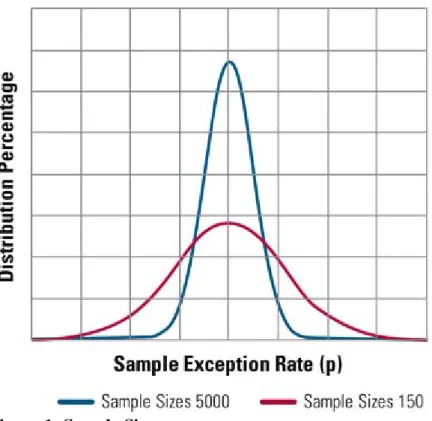
Given these definitions, the Central Limit Theorem says (in terms of our audit): If we draw multiple independent random samples of the same size n from a large book of recently underwritten cases and calculate the exception rate from each sample, then the pool of sample exception rates will be normally
distributed with a mean equal to p and a standard deviation equal to the square root of [(p * q) / n]. Figure 1 shows that the distribution of sample exception rates around the true population rate p is dependent upon the sample size. For a sample size of 5,000 there is only a small chance that a sample exception rate is very far off from the true rate shown by the value at the peak of each curve.
Figure 1: Sample Sizes
The larger your sample size, the more credible your sample.
Confidence Interval and Confidence Level
Before proceeding, we need to explain what is meant by two key parameters that need to be chosen by the underwriter before deciding upon an audit’s sample size. The confidence interval is a plus-or-minus percentage range surrounding the exception rate determined from the audit results. The plus-or-minus value is often called the sampling error.
The confidence level is the likelihood that the true rate inherent in the client’s entire book of business is somewhere in the confidence interval. For example, assume the results of an audit show a 15 percent exception rate. If the confidence interval is plus-or-minus two percent and the confidence level is 90 percent, then there is a 9 out of 10 chance that the book’s exception rate is between 13 and 17 percent. In other words, there is only a 10 percent chance that the client’s true exception rate is actually less than 13 or greater than 17 percent.
Determining the Sample Size
Now, we are ready to calculate the sample size. The “Z statistic” from a normal curve is used to determine the sampling error for a given confidence level. As a percent of sample size, the sampling error is equal to [Z * Sqrt (p * q) / Sqrt (n)]. Using a little algebra, we see that sample size equals [Z / (sampling error)]2 * p * (1 – p).
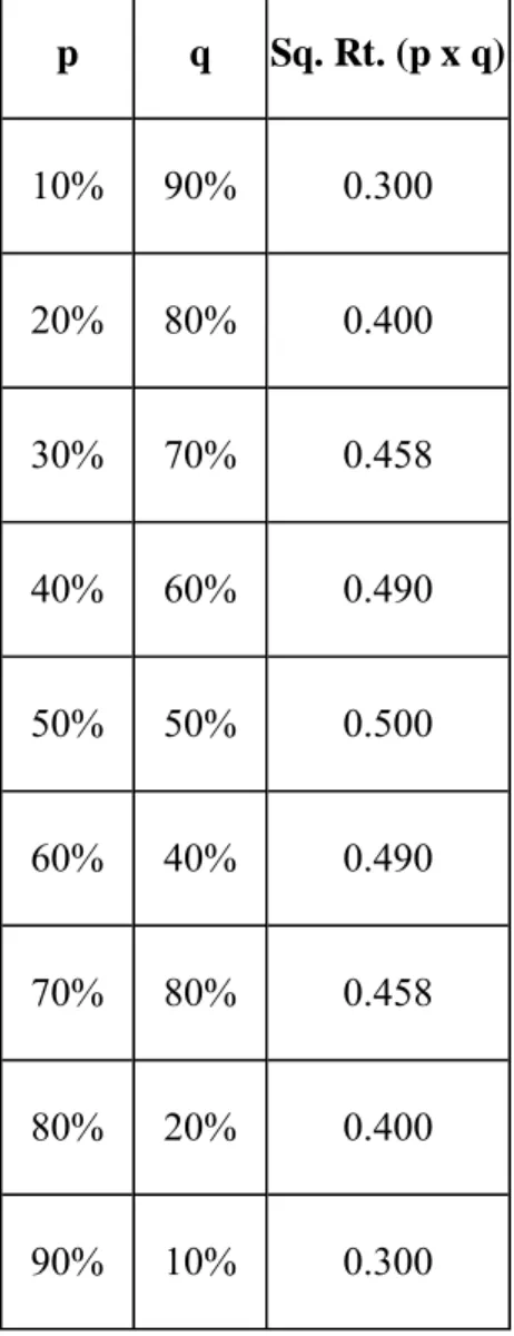
Unfortunately, this value depends on the exception rate p in the book, which we can’t estimate until we perform the audit. One popular and conservative approach is to use a value of p that produces the largest standard deviation and, therefore, the largest sample size. Figure 2 demonstrates that the largest standard deviation is produced when p is 50 percent.
p q Sq. Rt. (p x q) 10% 90% 0.300 20% 80% 0.400 30% 70% 0.458 40% 60% 0.490 50% 50% 0.500 60% 40% 0.490 70% 80% 0.458 80% 20% 0.400 90% 10% 0.300
Figure 2: Largest Standard Deviation
If you don’t (or can’t) know “p”, assuming it is 50 percent is the most conservative approach.
Our sample size formula is appropriate for populations of 20,000 and over. For smaller populations, an adjustment factor (beyond the scope of this article) can be incorporated into the formula. Figure 3 shows sample sizes for various combinations of confidence interval and confidence level for a large population using this approach.
Confidence Level Confidence Interval (+/- indicated percentage) 1.0% 2.0% 3.0% 4.0% 5.0% 10.0% 85.0% 5,181 1,295 576 324 207 52 90.0% 6,764 1,691 752 423 271 68 3 of 5 11/7/2011 1:45 PM
95.0% 9,604 2,401 1,067 600 384 96
99.0% 16,587 4,417 1,843 1,037 663 166
Figure 3: Conservative Sample Sizes for a Large Population
Smaller sample sizes may mean widening your confidence level or interval.
If previous knowledge or experience is available, it may be used to “guesstimate” the value of p in our sample size formula. Later, after audit results are in, we can adjust our final metrics with the true rate. This approach may result in a smaller or more practical sample size estimate and is the method we will use in the next section.
An Example of Sampling Theory in Action
We want to audit a large client’s book of recently underwritten business. The auditors want to review an appropriate number of cases so that they are confident the results are representative of the entire book. After discussions with client underwriters, the auditors want the exception rate determined by the audit to be within two percent of the client’s true rate with a 90 percent confidence level. Based upon prior audits, they estimate that the exception rate is likely to be around 10 percent. Figure 4 indicates that the auditors should review 591 cases. Having an estimate of the exception rate greatly reduces the
recommended sample size from the conservative value shown in Figure 3.
Input Parameters
Expected Response Rate 10% Population Size 20,000 Confidence Interval (+/-) 2.0%
Confidence Level 90.0%
Calculation Results
Recommended Sample Size 591
Figure 4: Pre-audit Metrics
Having a pre-audit estimate greatly reduces the recommended sample size.
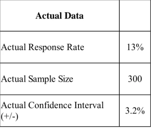
With pre-audit metrics in hand, the auditors proceed with their review but, due to time constraints, they only look at a random sample of 300 cases. The exception rate from these cases turns out to be 13
percent. We can now adjust the input parameters and determine the final audit metrics, shown in Figure 5.
Actual Data
Actual Response Rate 13% Actual Sample Size 300 Actual Confidence Interval
(+/-) 3.2%
Figure 5: Post-audit Adjusted Metrics
Increase the confidence interval to keep confidence level high, if the sample is short.
Given that audit results show an actual exception rate of 13 percent and knowing that we looked at 300 cases rather than the recommended 591, the confidence interval increases to a little over 3 percentage points. Thus, the auditors’ report indicates that they are 90 percent confident that the exception rate for entire book of recently underwritten business is between 10 and 16 percent.
Conclusion
While this article has discussed sampling theory in regards to an underwriting review, the results are equally valid for many other applications. The same concepts used by insurance auditors are also used by pollsters, television program rating services and quality control engineers. Understanding the limitations to measurements taken from a random sample gives us a better appreciation for why the results are always footnoted with a comment such as “sampling error is ±1.5 percentage points.”