A Stochastic Differential Equation for Modeling the Classical Probability Distributions

A Stochastic Differential Equation for

Modeling the “Classical” Probability Distributions

Greg Hertzler

School of Agricultural and Resource Economics Faculty of Natural and Agricultural Sciences

The University of Western Australia Crawley, 35 Stirling Highway, Perth, 6009

Email: [email protected].

Abstract

Stochastic differential equations are a flexible way to model continuous probability distributions. The most popular differential equations are for non-stationary Lognormal, non-stationary Normal and stationary Ornstein-Uhlenbeck distributions. The probability densities are known for these distributions and the assumptions behind the differential equations are well understood. Unfortunately, the assumptions do not fit most situations. In economics and finance, prices and quantities are usually stationary and positive. The Lognormal and Normal distributions are non-stationary and the Normal and Ornstein-Uhlenbeck distributions allow negative prices and quantities. This study derives a stochastic differential equation that includes most of the classical probability distributions as special cases and greatly expands the number distributions that can be used in models of stochastic dynamic systems.

Introduction

A continuous random variable can be modeled by a cumulative probability, a probability density or a stochastic differential equation. Of these, a differential equation is by far the most flexible. It can model an infinite variety of distributions, most with no known probability densities. Using stochastic calculus, it can combine with other differential equations to make a composite differential equation. This composite equation can be incorporated into a dynamic programming model to make optimal decisions for highly complex stochastic systems.

The flexibility of stochastic differential equations is a strength but also a weakness. The characteristics of the underlying probability distribution are not apparent. Is the distribution symmetric, allowing negative as well as positive values of the random variable? Or is the distribution asymmetric, imposing a lower bound, or an upper bound? Is the distribution strongly stationary with the random variable reverting to equilibrium? Is equilibrium at the mode, the mean or someplace else? Is the distribution weakly stationary with a changing equilibrium. Or is the distribution non-stationary with no equilibrium at all? Answers to these questions determine whether a particular distribution is appropriate for a particular situation. Answers are easy if the probability density is known.

For this reason, researchers tend to use differential equations that correspond to known probability densities. Three of the most popular are for non-stationary Lognormal, non-stationary Normal and stationary Ornstein-Uhlenbeck distributions.

(

)

. ; ; dz dt y b dy dz dt dy dz y dt y dy ρ µ ρ δ ρ δ + − − = + = + =

On the left-hand sides, dy is the stochastic change in random variable y. On the right-hand sides are expected changes and error terms. Expected changes include time interval dt and error terms include a Weiner increment dz. Thus y is a random variable because its differential equation transforms a Weiner increment into a stochastic change over time. The distribution of y is determined by the transformation.

Which differential equation corresponds to which probability distribution? It is not apparent that the first equation is for a Lognormal distribution in which random variable y must be non-negative, nor that the second two equations are for Normal and Ornstein-Uhlenbeck distributions in which y can be negative or positive. It is apparent that the first equation assumes exponential growth, the second equation assumes linear growth and the third equation may have a stochastic equilibrium where random variable y reverts to location parameter µ. It is not apparent that µ is the mode and also the mean. The first two equations have rate δ and scale parameter ρ. It is not apparent that these are

time derivatives of linear functions. Finally, the third equation has rate b and scale ρ. It is not apparent that b is a simple parameter but ρ is an asymptotic function of time plus its time derivative.

All three equations are more complex than they seem. All three have been used as models of random prices. Are they appropriate models? Surely prices cannot be negative, which disqualifies the second and third equations. Stock prices may grow exponentially, but commodity prices do not. Consequently, the first equation may be appropriate for some prices but not others. Whether appropriate or not, these three equations are used because they appear simple and their distributions are known. Appropriate models could be used if differential equations for more of the classical probability distributions could be found. The purpose of this study is to find them.

Inventing a stochastic differential equation is easy but finding the equation that corresponds to a probability density requires persistence and a bit of luck. The next section introduces methods that may improve the odds and demonstrates with simple examples. Then follows the main result: a differential equation that includes most of the classical distributions as special cases. Finally, the special cases are defined and discussed.

Stochastic Differential Equations for Probability Densities

A cumulative probability counts the proportion of time a random variable is less than some limit; a probability density counts the proportions of time a random variable spends at each of its possible values; and a stochastic differential equation measures how a random variable changes over time. Just as a probability density is the derivative of a cumulative probability, a stochastic differential equation satisfies derivative properties of the probability density. These derivative properties are two partial differential equations called the Kolmogorov forward and backward equations (Grimmett and Strizaker, 1997, p. 494). A stationary process must satisfy the Kolmogorov forward equation and a non-stationary process must satisfy the backward equation as well.

A non-stationary process has no equilibrium. Instead, forward variable y, at forward time t, is measured against backward variable x, at backward time s. Change y – x occurs over time interval t –

s. The cumulative probability and probability density are functions of the forward and backward

variables but the stochastic differential equation is a function only of the forward variables.

(

)

(

)

( )

,

( )

, . ; , , , ; , , , dz t y h dt t y g dy s x t y f s x t y F + =

F is the cumulative probability, f is the probability density and dy is the stochastic change in y.

Expected change gdt, where g is drift, will be in error by hdz, where h is the standard deviation and dz is a Weiner increment. Given the cumulative probability and probability density, functions g and h are chosen to satisfy the Kolmogorov forward and backward equations:

( )

[

( )

]

[

( )

]

( )

,

( )

, 0. ; 0 , , 1 2 2 2 2 1 2 2 2 2 1 = ∂ ∂ + ∂ ∂ + ∂ ∂ = ∂ ∂ − ∂ ∂ + ∂ ∂ x f t x h x f s x g s f y f t y h y f t y g t f

The forward equation is evaluated with forward variables y and t in functions g and h. The backward equation, however, is evaluated with backward variables x and s substituted in for the forward variables. These equations may be difficult to satisfy. If f is known, g and h may be hard to find. It is easy to choose g and h, but f may be hard to find. Lognormal and Normal distributions are the most common examples. As shown below, the Ornstein-Uhlenbeck process can also be non-stationary.

Stationary processes can be categorized into strongly stationary and weakly stationary. Often Weakly stationary processes are often defined to have a constant mean but a changing variance (Grimmett and Strizaker, 1997, p. 333). Here, a weakly stationary process is defined to have an equilibrium that changes over time. The cumulative probability and probability density are functions of the forward variables only.

( )

( )

( )

,

( )

, . ; , ; , dz t y h dt t y g dy t y f t y F + =

The backward equation has a trivial solution and functions g and h are chosen to satisfy the forward equation.

( )

2

[ ]

[ ]

0. 2 2 2 2 1 = ∂ ∂ − ∂ ∂ + ∂ ∂ y f h y gf t f

Finding functions g and h for weakly stationary processes is easier than for non-stationary processes, but still challenging.

A strongly stationary process has a fixed. The cumulative probability, probability density and differential equation are functions of the random variable but not of time.

( )

( )

( )

( )

. ; ; dz y h dt y g dy y f y F + =

The backward equation has a trivial solution and the forward equation no longer has a time derivative.

( )

3

[ ]

[ ]

0. 2 2 2 2 1 = ∂ ∂ − ∂ ∂ y f h y gf

It is easy to find a differential equation for a strongly stationary process. In fact it is easy to find several versions of its differential equation. First choose diffusion, h2, as the square of the standard deviation, and rewrite the probability density as a constant, C, multiplied by an auxiliary function, φ, and divided by diffusion.

( )

( )

( )

2. y h y C y f = φ

Drift g is defined by diffusion and the corresponding auxiliary function.

( )

1₂ 2 . φ φ y h y g = ∂ ∂

To check that the forward equation is satisfied, first note that equation (3) can be integrated into a simpler form.

[ ]

2 _0. 2 1 = ∂ ∂ − y f h gf

Also, rearrange the formula for drift to solve for the derivative of the auxiliary function. . 2 ₂φ φ h g y = ∂ ∂

Finally, evaluate the forward equation.

[ ]

_0. 2 2 1 2 2 1 = − = − = ∂ ∂ − = ∂ ∂ − gf gf h gC gf y C gf y f h gf φ φ

Example: Strongly Stationary Gamma Distribution

The Gamma density is one of the special cases discussed below. Consider its stationary probability density.

( )

(

)

( )

0 ; . ; 0 ; 0 ; 1 ∞ < < < < < Γ − = − − − y b e y b y f y b µ σ α σ α µ _σµ α α α

Parameter α is the shape parameter, µ is the location parameter and σ and b are scale parameters. Parameter b is redundant in the probability density but will become the rate of decrease toward equilibrium in the differential equation. Many versions of a stochastic differential equation are possible. Three examples have constant, linear and quadratic diffusion.

Constant Diffusion

( ) (

)

₍

(

)

₎

( )

(

1

)(

)

. . 1 ; . 2 1 1 2 σ µ α φ σ µ α φ µ φ σ σµ α − − − − − − + − = − − − = ∂ ∂ − = = y b y g b y y e y y h y b Linear Diffusion

( )

(

)

( ) (

)

( )

(

)

. . ; . 2 2 ασ µ φ σ µ α φ µ φ σ µ σµ α + − − = − − = ∂ ∂ − = − = − − y b y g b y y e y y y y h y b

Quadratic Diffusion

( )

(

)

( ) (

)

( )

(

) (

1

)(

)

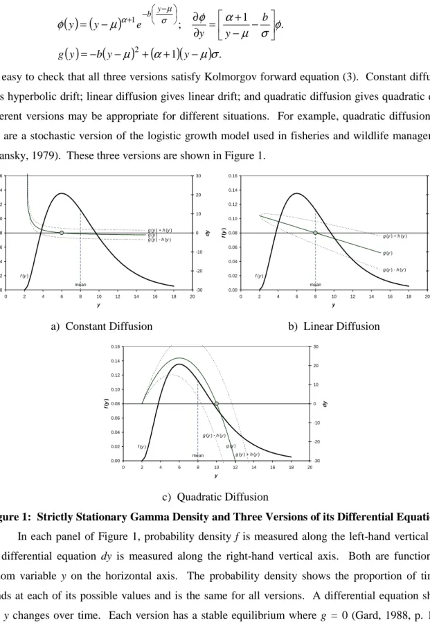
. . 1 ; . 2 2 1 2 2 σ µ α µ φ σ µ α φ µ φ σ µ σµ α − + + − − = − − + = ∂ ∂ − = − = − − + y y b y g b y y e y y y y h y b

It is easy to check that all three versions satisfy Kolmorgov forward equation (3). Constant diffusion gives hyperbolic drift; linear diffusion gives linear drift; and quadratic diffusion gives quadratic drift. Different versions may be appropriate for different situations. For example, quadratic diffusion and drift are a stochastic version of the logistic growth model used in fisheries and wildlife management (Polansky, 1979). These three versions are shown in Figure 1.

f (y ) mean g (y ) g (y ) + h (y ) g (y ) - h (y ) 0.00 0.02 0.04 0.06 0.08 0.10 0.12 0.14 0.16 0 2 4 6 8 10 12 14 16 18 20 y f (y ) -30 -20 -10 0 10 20 30 d y f (y ) mean g (y ) g (y ) + h (y ) g (y ) - h (y ) 0.00 0.02 0.04 0.06 0.08 0.10 0.12 0.14 0.16 0 2 4 6 8 10 12 14 16 18 20 y f (y ) -30 -20 -10 0 10 20 30 d y

a) Constant Diffusion b) Linear Diffusion

f (y ) mean g (y ) g (y ) + h (y ) g (y ) - h (y ) 0.00 0.02 0.04 0.06 0.08 0.10 0.12 0.14 0.16 0 2 4 6 8 10 12 14 16 18 20 y f (y ) -30 -20 -10 0 10 20 30 d y c) Quadratic Diffusion

Figure 1: Strictly Stationary Gamma Density and Three Versions of its Differential Equation.

In each panel of Figure 1, probability density f is measured along the left-hand vertical axis and differential equation dy is measured along the right-hand vertical axis. Both are functions of random variable y on the horizontal axis. The probability density shows the proportion of time y spends at each of its possible values and is the same for all versions. A differential equation shows how y changes over time. Each version has a stable equilibrium where g = 0 (Gard, 1988, p. 133). After a random shock, constant diffusion reverts to the mode; linear diffusion reverts to the mean; and quadratic diffusion reverts to equilibrium above the mean. Quadratic diffusion also has an unstable equilibrium at the lower bound imposed by the location parameter.

All versions must spend the same proportion of time at each value of y. For example with linear and quadratic diffusion, y spends more time at the mode than in equilibrium. This is explained by graphing g plus and minus one standard deviation, h. At equilibrium, a random shock is equally likely to decrease y as to increase it. However, below equilibrium, y is more likely to increase. Above equilibrium, y is more likely to decrease. With linear and quadratic diffusion, standard deviations increase as y increases. Above equilibrium, y is likely to decrease quickly, perhaps overshooting equilibrium and spending time around the mode. Below equilibrium, y is likely to increase more slowly, again spending time around the mode.

Equilibrium at the mode is intuitively appealing and not unique to the Gamma distribution. With constant diffusion, drift can be defined directly using the probability density instead of the auxiliary function.

( )

1₂ 2 . f y f h y g = ∂ ∂

Equilibrium, where g = 0, is at the mode, where ∂f ∂y=0. If diffusion is constant, equilibrium is at the mode for any strongly stationary distribution.

Example: Weakly Stationary Gamma Distribution

Suppose equilibrium changes because the location and scale parameters are functions of time.

( )

(

( )

)

( ) ( )

( ) ( ) . ; 0 ; 0 ; 0 ; , 1 ∞ < < < < < Γ − = − − − y b e t t y b t y f t t y b µ σ α σ α µ σµ α α α

Kolmogorov forward equation (2) includes the time derivative of f.

(

)

₂ 1 f. t b y f t y b f t t f ∂ ∂ − − − − ∂ ∂ − + ∂ ∂ − = ∂ ∂ µ σ µ α σ σ µ σ σ α

The time derivative restricts the powers of y that can be included in diffusion and drift. Trial and error shows that weakly stationary counterparts to constant and quadratic diffusion do not satisfy the Kolmogorov forward equation. Fortunately, a counterpart to linear diffusion does.

( )

(

)

( )

. ; 2 , 2 t b t t g b t y t y h ∂ ∂ + ∂ ∂ = ∂ ∂ − = µ σ α σ µ

There is only one version of the differential equation for weakly stationary distributions and it may be difficult to find. First finding strongly stationary versions will narrow the search to a few likely candidates.

Example: Stationary Gamma Distribution

Diffusion and drift for a strongly stationary distribution also satisfy the Kolmogorov forward equation for a weakly stationary distribution. Thus, diffusion and drift can be a combination of

( )

(

)

( )

,

(

)

. ; 2 , 2 t b t y b t y g b t y t y h ∂ ∂ + ∂ ∂ + + − − = ∂ ∂ + − = µ σ σ α µ σ σ µ

If location and scale are constant, diffusion and drift become strongly stationary. If either location or scale changes over time, equilibrium also changes.

The square root of diffusion becomes the standard deviation in a differential equation for the stationary Gamma distribution.

( )

4

(

)

2

(

)

. 2 1 2 1 2 1 dz b t y dt t dt b t dt y b dy ∂ ∂ + − + ∂ ∂ + ∂ ∂ + + − − = µ α σ σ µ µ σ σ

Particular functional forms for location and scale will simplify equation (4). Suppose location is constant and scale approaches an asymptote.

( )

[

1

]

; . ; 0 ρ σ σ ρ σ µ = ∂ ∂ + − = = ∂ ∂ − b t ce t t bt

With these assumptions, the stationary version of the differential equation is indistinguishable from the strongly stationary version.

(

_y

)

_{dt dt} 212

(

_y

)

12 12_dz.

b

dy=− −µ +αρ + −µ ρ

This equation is suitable for random variables such as commodity prices and quantities that are bounded below and tend toward equilibrium. A differential equation for a stationary Lognormal distribution could be derived in the same way and would also be suitable.

Example: Stationary and Non-stationary Ornstein-Uhlenbeck Process

The Ornstein-Uhlenbeck process can be either stationary or non-stationary. First consider a stationary probability density.

( )

( )

( ) ( ) . ; 0 ; 0 ; , 2 2 1 2 1 ∞ < < ∞ − < < = − − y b e t b t y f t t y b σ σ π σµ

As a guess, try constant diffusion for both strongly and weakly stationary versions.

( )

( )

,

(

)

. ; 2 , 2 2 2 t y b t y g b t t y h ∂ ∂ + − − = ∂ ∂ + = µ µ σ σ

Fortunately, Kolmogorov forward equation (2) is satisfied. Taking the square root of diffusion gives the differential equation for the Ornstein-Uhlenbeck process in a general form.

( )

(

)

. 2 5 2 1 2 2 dz b t dt t dt y b dy ∂ ∂ + + ∂ ∂ + − − = µ µ σ σ

( )

[

]

. 2 ; 1 ; 0 2 2 2 2 2 2 _{ρ σ} σ _ρ σ µ = ∂ ∂ + − = = ∂ ∂ − b t ce t t bt

This gives the more familiar differential equation for a stationary Ornstein-Uhlenbeck process.

(

y

)

dt dz.

b

dy=− −µ +ρ

This equation is suitable for random variables that can be negative as well as positive and tend toward equilibrium. Setting b to 1_{2 gives a stationary Normal distribution.}

Now consider a non-stationary probability density.

(

)

( )

( ) ( ) . ; 0 ; 0 ; , , , 2 2 1 2 1 ∞ < < ∞ − < < − = − − − − − y b e s t b s x t y f t s s t x y b σ σ π σ µ

Forward variable y is replaced by difference y – x and forward time t is replaced by interval t−s, where x and s are backward variables. As a guess, try the weakly stationary version of diffusion and drift.

( )

( )

, . ; 2 , 2 2 t t y g b t t y h ∂ ∂ = ∂ ∂ = µ σ

Luckily, the Kolmogorov forward and backward equations in (1) are both satisfied. To simplify, suppose location and scale are constants multiplied by time interval t−s.

( )

[ ]

( )

[ ]

. 2 2 ; ; ; 2 2 2 2 b b t s t s t t s t s t ρ σ ρ σ δ µ δ µ = ∂ ∂ − = − = ∂ ∂ − = −

These assumptions give a very simple differential equation for the non-stationary Ornstein-Uhlenbeck process.

( )

2_b 12 _dz.

dt

dy=δ + − ρ

This equation is suitable for random variables that can be negative or positive and that grow linearly over time. Setting parameter b to 1_{2 gives the familiar differential equation for a non-stationary}

Normal distribution.

Although a differential equation may be simple and appealing, it may or may not be appropriate. Assumptions are embedded within it by the probability density, by the location and by the scale. In the next section, a stochastic differential equation is found that corresponds to a flexible functional form for the probability density and arbitrary functions for the location and scale. It includes most of the classical probability distributions as special cases. At least one special case should be appropriate for any particular situation.

Beta Family of Differential Equations

Generalized probability distributions are flexible models of random variables. The Generalized Hypergeometric distribution is one of the most general. It is defined using a hypergeometric series and includes many of the classical probability distributions as special cases. Here, a simpler generalization will also include the classical probability distributions. This generalization will be called the Beta Family of distributions. The cumulative probability and probability density of stationary random variable y at time t are:

( )

( )

(

,

)

( )

(

( )

)

1

( )

( )

. , 6 1 dv t t v a b t v t a a b t y F a y − −

∫

− + − − Β = µ β α α β α β α σ µ µ σ β β α β α

( )

( )

(

( )

)

(

)

( )

( )

( )

. ; 0 ; 0 ; 1 ; ; 1 ; 0 ; 0 : with ; 1 , , 7 1 ∞ < < < < < < + ≤ < < − + − Β − = − − y b a a t t y a b t a a t y b t y f a µ σ α β β α σ µ σ µ β β α β α β α β α α β α β α

There are six parameters. Parameters a and b will be called family parameters. The Generalized Gamma and Generalized Beta II distributions are special cases as a goes to infinity and a = b, respectively. Parameters α and β are shape parameters. Specific values of these give further special cases such as the Gamma, Weibull, Exponential, Chi-square, F, Burr XII, and Pareto II distributions. Parameters µ and σ are the location and scale parameters. The location parameter sets a lower bound and the scale parameter determines the dispersion of the distribution. Both location and scale can be functions of time. Restrictions on the parameters ensure that the cumulative probability, the probability density and the differential equation, to be derived below, all exist. For example, the beta function, Β (see Appendix 4) requires its arguments to be positive.

The generalization that creates the Beta Family is the additional parameter b. In the cumulative probability and probability density, this parameter is indistinguishable from the scale parameter, σ. However in the differential equation, b is the rate of decrease toward equilibrium. A stochastic differential equation satisfying Kolmogorov forward equation (2) is:

( )

( )

( )

( )

(

) (

)(

)

( )

(

)

. 1 1 2 , ; 1 1 1 , : where ; , , 8 2 1 2 1 2 1 2 2 1 2 1 2 1 − − + ∂ ∂ + − = ∂ ∂ + − − + ∂ ∂ + − − + + − − = + = − − a a y a b b t y t y h t a a y a b b t y y b t y g dz t y h dt t y g dy β β β β β β β σµ β σ β σ µ µ σµ β σ β σ µ β α µ β

Proof is in Appendix 2. Equation (8) is the main result of this study. It includes the most commonly used distributions as special cases and greatly expands the choice of distributions for use in dynamic decision models. Interestingly, the differential equation has more special cases than do the cumulative

probability and density function. It is not encumbered by limits of integration nor by a constant of integration. Distributions with no lower bound, such as the Ornstein-Uhlenbeck discussed above, and distributions with both lower and upper bounds, such as the Beta to be discussed below, are also special cases.

Standardized moments of the Beta Family are derived in Appendix 3.

( )

( )

( ) (

)

( ) (

)

; 0 . 9 β α σµ α_β α_β β α β α β β − < ≤ − Γ Γ − Γ Γ = − = + + i a a b a a y E i M _i i i i i

Function M(i) is not a moment generating function. Rather it directly calculates the ith moment of the standardized variable, (y – µ) / σ. Moment M(0) always exists and equals one because the cumulative probability in equation (6) approaches one as y goes to infinity. Higher moments, such M(1) and M(2) may or may not exist. If i = aβ – α, the argument of the gamma function, Γ (see Appendix 4) is zero and the gamma function goes to infinity. Below this, i can be a nonnegative real number, although usually it will be integer. Also derived in Appendix 3 is the incomplete moment function, M( yi, ), for a distribution truncated at y . The 0th incomplete moment is the cumulative probability in equation (6), and the 0th and 1st incomplete moments can be used for pricing of insurance and options.

The stochastic differential equation may or may not revert to the mean. Setting g = 0 in equation (8) and rearranging gives the equilibrium.

(

)

(

)

. 1 1 1 β α β α β σµ − − − + = − a b a y

Setting β = 1 in equation (9) and applying the factorial property of the Γ function (see Appendix 4) simplifies the 1st moment.

( ) (

)

. 1 1 − − = α α a b a M

Except for symmetric distributions to be discussed below, the differential equation reverts to the mean of the Beta Family so long as β = 1. If β < 1, equilibrium is above the mean and if β > 1, equilibrium

is below the mean. If β = 1 + α, equilibrium is at the lower bound set by the location parameter, µ. These cases are shown in Figure 2. As before, the density is measured by the vertical axis on the left-hand side and the differential equation is measured by the vertical axis on the right-left-hand side. Both are functions of y on the horizontal axis. In each case, there is a stable equilibrium. However, y is stochastic and spends less time in equilibrium than elsewhere. At the extreme, y spends no time at all in equilibrium if that equilibrium is at the lower bound.

f(y ) mean g (y ) g (y ) + h (y ) g (y ) - h (y ) 0.00 0.02 0.04 0.06 0.08 0.10 0.12 0.14 0.16 0 2 4 6 8 10 12 14 16 18 20 y f (y ) -30 -20 -10 0 10 20 30 d y f(y ) mean g (y ) g (y ) + h (y ) g (y ) - h (y ) 0.00 0.02 0.04 0.06 0.08 0.10 0.12 0.14 0.16 0.18 0 2 4 6 8 10 12 14 16 18 20 y f (y ) -30 -20 -10 0 10 20 30 d y a) β <1. b) β = 1. f(y ) mean g (y ) g (y ) + h (y ) g (y ) - h (y ) 0.00 0.05 0.10 0.15 0.20 0.25 0.30 0 2 4 6 8 10 12 14 16 18 20 y f (y ) -30 -20 -10 0 10 20 30 d y f(y ) mean g (y ) g (y ) + h (y ) g (y ) - h (y ) 0.00 0.02 0.04 0.06 0.08 0.10 0.12 0.14 0 2 4 6 8 10 12 14 16 18 20 y f (y ) -30 -20 -10 0 10 20 30 d y c) β > 1. d) β = 1 + α

Figure 2: Beta Family Equilibrium Above, At and Below its Mean and at its Lower Bound.

As before, assuming a constant location and an asymptotic function for scale makes the stationary version in equation (8) indistinguishable from a strongly stationary version.

(

1

)

; . ; 0 2 ρ β σ β σ βρ σ µ β β β β _{= − +}∂ ∂ ₌ = ∂ ∂ − b t ce t t b

Even with this simplification, equation (8) is flexible but complicated. The special cases discussed in the next section are simpler.

Special Cases

Special cases of the Beta Family are diagrammed in Figure 3. The Generalized Gamma, the Generalized Beta II and the F distribution have limits of integration of µ< y<∞ and are special cases of the cumulative probability in equation (6) and the probability density in equation (7). These distributions are also special cases of differential equation (8). The Generalized Gamma and Generalized Beta II are very similar and have further special cases, as shown in Figure 3. Of the special cases, the Gamma and the Beta-prime distributions are similar; the Weibull and Burr XII are similar and the Exponential and Pareto II are similar. Also, the F and Chi-square distributions are similar.

The differential equation also includes the Generalized Student t and the Generalized Beta I distributions as special cases. As shown in panel a) of Figure 4, the Generalized Student t has a symmetric probability density with limits of integration of −∞< y<∞. Its differential equation reverts to a stable equilibrium at location parameter µ which equals the mode and the mean. The Generalized Student t has the Ornstein-Uhlenbeck, Student t and Normal distributions as important special cases. As shown in panel b) of Figure 4, the Generalized Beta I has a probability density with both lower and upper bounds and limits of integration of µ<y<µ+σ . It differential equation has a stable equilibrium above the mean if parameter β < 1, at the mean if β = 1, lower than the mean if β >

1 and at the lower bound if β = 1+ α. The Generalized Beta I has the Beta, Power and Uniform distributions as important special cases.

f(y ) mean g (y ) g (y ) + h (y ) g (y ) - h (y ) 0.00 0.02 0.04 0.06 0.08 0.10 0.12 0.14 0.16 -6 -4 -2 0 2 4 6 8 10 y f (y ) -30 -20 -10 0 10 20 30 d y f(y ) mean g (y ) 0.00 0.05 0.10 0.15 0.20 0.25 0.30 0.35 0.40 0.45 0.50 0 1 2 3 4 5 6 7 y f (y ) -30 -20 -10 0 10 20 30 d y

a) Generalized Student t b) Generalized Beta I.

Figure 4: Equilibrium with No Lower Bound and with Both Lower and Upper Bounds.

Differential equations for two special cases, the Gamma and Ornstein-Uhlenbeck distributions, were derived above in equations (4) and (5). These and the other special cases are defined in Appendix I. Proof for each special case follows from the proof for the Beta Family in Appendix 2. Although the constants of integration differ, the variable portion of each probability density is a special case of equation (7). Therefore the derivatives of density f, drift g and diffusion h2 are special cases of those for the Beta Family, the Kolmogorov forward equation (2) is satisfied and each differential equation is a special case of equation (8).

Other special cases are not shown in Figure 3. As examples, the Generalized Chi has the Chi, Helmert and Maxwell-Boltzmann distributions as special cases. The Gamma has the Erlang; the Student t has the Cauchy; the Beta has the Triangular II and the Power has the Triangular I as special cases.1 Many distributions have other names.2 For consistency, the names used here follow the

1 _Chi

(

)

2 ; ; 2 ; _{n b} n a→∞ β = α= = ; Helmert

(

_a→∞;β =2;α =_n−1;_b=n₂

)

_{; Maxwell-Boltzmann}

(

a→∞;β =2;α =3

)

; Erlang

(

a→∞;β =1;α =n

)

; Cauchy

(

2; 1;

(

1

)

; 1 ; 1

)

2 1 + = → = = = α a n b a _n n β ; Triangular II

(

a=−b;β =1;α =2;b→0

)

; Triangular I

(

a=b;β =1;α =1;b=1

)

.

2 _{Gamma (Pearson III); Weibull (Weibull-Gnedenko, Rosin-Rommler); Student t (Pearson VII); Normal}

(Gaussian); F (Snedecor F); Beta (Beta I, Pearson I); Uniform (Rectangular); Generalized Beta II (Generalized F, Feller-Pareto); Burr XII (Beta-P, Singh-Maddala); Beta-Prime (Beta II, Pearson VI); Pareto II (Lomax);

nomenclature of Johnson, Kotz and Balakrishnam (1994; 1995) except, perhaps, for the name Generalized F which is often used instead of Generalized Beta II. Five of the special cases in Figure 3 are unnamed and apparently unstudied in the literature. One of these five has been dubbed the ‘Single Shape’ distribution because shape parameter α is set equal to shape parameter β. It generalizes those distributions with an analytical solution for the cumulative probability, including the Weibull, Exponential, Rayleigh, Power, Uniform, Burr XII and Pareto II distributions. Most distributions have small, positive integers for the shape parameters. Larger, negative or non-integer values are possible, giving an infinity of special cases for the Beta Family.

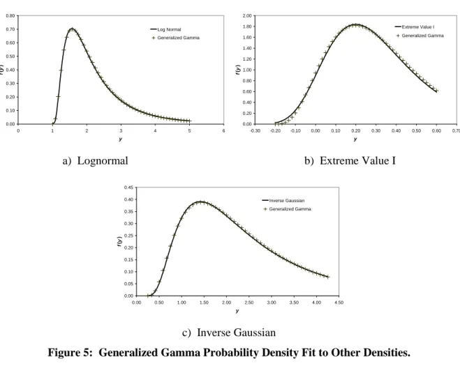
Three important distributions are not special cases, however. The Lognormal distribution can become a special case of the Generalized Gamma distribution if the parameters are redefined so that the limit exists as β goes to zero. The Extreme Value I distribution is a special case of the Gamma distribution only if (y – µ) / σ is replaced by exp((y – µ) / σ). The Inverse Gaussian distribution cannot be transformed into a special case of the Beta Family. As shown in Figure 5, however, the probability density for the Generalized Gamma distribution can empirically fit the densities for the Lognormal, Extreme Value I and Inverse Gaussian distributions.

0.00 0.10 0.20 0.30 0.40 0.50 0.60 0.70 0.80 0 1 2 3 4 5 6 y f (y ) Log Normal Generalized Gamma 0.00 0.20 0.40 0.60 0.80 1.00 1.20 1.40 1.60 1.80 2.00 -0.30 -0.20 -0.10 0.00 0.10 0.20 0.30 0.40 0.50 0.60 0.70 y f (y ) Extreme Value I Generalized Gamma

a) Lognormal b) Extreme Value I

0.00 0.05 0.10 0.15 0.20 0.25 0.30 0.35 0.40 0.45 0.00 0.50 1.00 1.50 2.00 2.50 3.00 3.50 4.00 4.50 y f (y ) Inverse Gaussian Generalized Gamma c) Inverse Gaussian

The Generalized Beta II is similar to the Generalized Gamma and can also fit the probability densities in Figure 5. The Generalized Student t can fit symmetric densities that are unbounded and the Generalized Beta I can fit densities with both lower and upper bounds.

Potential Applications

The Beta Family is a set of flexible functional forms that can model the classical probability distributions. Random variables are assumed to be strongly stationary, reverting to a fixed equilibrium, or weakly stationary, reverting to a time-varying equilibrium. Two special cases, the Ornstein-Uhlenbeck and Normal distributions, can also be non-stationary with no equilibrium. Many, if not most, random variables are stationary, however, and members of the Beta Family will be appropriate for many situations.

For example, in finance, the non-stationary Lognormal distribution is used extensively because it has a simple differential equation. However, it consistently underestimates the volatility of prices. One of the remedies is to modify the differential equation and rename it a Constant Elasticity-of-Variance equation. . 2 _dz y dt y dy= δ + c− ρ

Prices are assumed to be non-stationary and grow exponentially at rate δ. Otherwise, the probability distribution is unknown. A differential equation for the Generalized Gamma distribution could be used instead.

(

1

)

_y1 _dt 212_y1 2 12_dz.

dt by

dy=− + +α−β −βρ + −β ρ

Prices would have a constant elasticity-of-variance and would be stationary and nonnegative. In addition, this differential equation is more flexible and likely to better fit the data.

Stochastic differential equations are extremely flexible and can model probability distributions that have no known probability densities. Unless the probability density is known, however, the characteristics of that distribution are not apparent. Interpreting models is difficult. Parameter estimation becomes a challenge because traditional techniques such as the method of moments and maximum likelihood require knowledge of the probability density. An active area of research is developing new methods for estimating stochastic differential equations. Members of the Beta Family can be used in this research to generate pseudo-data for several known probability densities. Then the parameters of differential equations can be estimated. Finally, the estimated parameters can be compared with the true parameters to test for bias and efficiency.

References

Gard, Thomas C. (1988) Introduction to Stochastic Differential Equations, New York, Marcel Dekker, Inc.

Grimmett, G. R., and Strizaker, D. R. (1997) Probability and Random Processes, second edition, Oxford, Clarendon Press

Johnson, Norman L., Kotz, Samuel and Balakrishnan, N. (1994) Continuous Univariate Distributions:

Volume 1, second edition, New York, John Wiley & Sons, Inc.

Johnson, Norman L., Kotz, Samuel and Balakrishnan, N. (1995) Continuous Univariate Distributions:

Volume 2, second edition, New York, John Wiley & Sons, Inc.

Polansky, P. (1979) "Invariant distributions for multi-population models in random environments"

Theoretical Population Biology 16:24-34.

Appendix 1: Special Cases

Generalized Gamma (a→∞)

( )

_{( )}

( )

(

( )

)

( ) ( ) _. , v t 1e dv t b t y F t t v b y β β α σµ µ α α β α _σ µ β − − −

∫

− Γ =

( )

_{( )}

(

( )

)

( )

( ) ( ) . ; 0 ; 0 ; 1 ; 0 ; 0 ; , 1 ∞ < < < < + ≤ < < Γ − = − − − y b e t t y b t y f t t y b µ σ α β β α σ µ β β β α σµ α β α α

( )

(

) (

)(

)

( )

, 2

(

)

. ; 1 , 2 1 2 2 1 2 1 2 1 ∂ ∂ + − = ∂ ∂ + ∂ ∂ + − − + + − − = − − β σ β σ µ µ β σ β σ µ β α µ β β β β β β b t y t y h t b t y y b t y g

( )

( )

( )

; 0 i. b i M _i i ≤ Γ Γ = + β α β α β Gamma (a→∞;β =1)

( )

( ) ( )

(

( )

)

( ) ( ) _. , v t 1e dv t b t y F t t v b y − − −

∫

− Γ = σ µ µ α α α µ σ α

( )

(

( )

)

( ) ( )

( ) ( ) . ; 0 ; 0 ; 0 ; , 1 ∞ < < < < < Γ − = − − − y b e t t y b t y f t t y b µ σ α σ α µ σµ α α α

( )

(

)

( )

, 2

(

)

. ; , 2 1 2 1 2 1 !"# ∂ ∂ + − = ∂ ∂ + !"# ∂ ∂ + + − − = b t y t y h t b t y b t y g σ σ µ µ σ σ α µ

( ) (

)

( )

; 0 i. b i i M i_Γ ≤ + Γ = α α

Branching Process (a→∞;β =1;α →0)

( )

_,

(

( )

)

1 ( )( ) _. dv e t v t y F t t v b y − − −

∫

− = σ µ µ µ

( )

, =

(

−

( )

)

1 ( )( ) ; 0< ; < <∞. − − − _{e y} t y t y f t t y b µ σ µ σ µ

( )

(

)

( )

, 2

(

)

. ; , 2 1 2 1 2 1 ∂ ∂ + − = ∂ ∂ + − − = b t y t y h t y b t y g σ σ µ µ µ

( ) ( )

; 0 i. b i i M =Γ_i ≤ Exponential (a→∞;β =1;α =1)

( )

_{, 1} ( )( ) _. − − − = t t y b e t y F σ µ

( )

_{, =}

_{( )}

( )( ) _{; 0< ; < <∞.} − − y e t b t y f t t y b µ σ σ σ µ

( )

(

)

( )

, 2

(

)

. ; , 2 1 2 1 2 1 !"# ∂ ∂ + − = ∂ ∂ + !"# ∂ ∂ + + − − = b t y t y h t b t y b t y g σ σ µ µ σ σ µ

( ) ( )

1 ; 0 i. b i i M =Γ +_i ≤ Chi-square ( 1₂ 2; ; 1 ; = = = ∞ → b a β α k ₎

( )

( )

( )

(

( )

)

( ) ( ) _. 2 1 , 2 1 2 2 2 1 2 dv e t v t t y F t t v y k k k k $ $ %& ' '() − − −

∫

− Γ = σ µ µ µ σ

( )

(

( )

)

( )

( )

( ) ( ) . ; 0 ; , 3 , 2 , 1 ; 2 , 2 1 2 2 2 2 1 ∞ < < < = Γ − = * * +, --./ − − − y k e t t y t y f t t y k k k k µ σ σ µ σµ 0

( )

(

)

(

)

( )

, 2

(

) (

2

)

. ; 2 , 2 1 2 1 2 1 2 2 1 t y t y h t t y t y g k ∂ ∂ + − = ∂ ∂ + ∂ ∂ + + − − = σ σ µ µ σ σ µ

( )

2

(

_{( )}

)

; 0 . 2 2 i _i i M k k i ≤ Γ + Γ = Weibull (a→∞;α =β)

( )

_{, 1} ( )( ) _. β σ µ 1 1 23 4 456 − − − = t t y b e t y F

( )

(

( )

)

( )

( ) ( ) . ; 0 ; 0 ; 0 ; , 1 ∞ < < < < < − = − − − y b e t t y b t y f t t y b µ σ β σ µ β β σµ β β

( )

(

) (

)

( )

, 2

(

)

. ; , 2 1 2 2 1 2 1 2 1 ∂ ∂ + − = ∂ ∂ + ∂ ∂ + − + − − = − − β σ β σ µ µ β σ β σ µ µ β β β β β β b t y t y h t b t y y b t y g

( )

(

1

)

; 0 i. b i M _i i ≤ + Γ = β β Generalized Chi (a→∞;β =2)

( )

( )

( )

(

( )

)

( ) ( ) _. 2 , 2 2 1 2 dv e t v t b t y F t t v b y − − −

∫

− Γ = σ µ µ α α α _σ µ α

( )

(

_{( )}

( )

)

( )

( ) ( ) . ; 0 ; 0 ; 1 ; 2 , 2 2 2 1 ∞ < < < < < Γ − = − − − y b e t t y b t y f t t y b µ σ α σ µ σµ α α α α

( )

(

) (

)(

)

( )

. 2 , ; 4 2 1 , 2 1 2 2 2 2 1 ∂ ∂ + = ∂ ∂ + ∂ ∂ + − − + − − = − b t t y h t b t y y b t y g σ σ µ σ σ µ α µ

( )

( )

( )

2 ; 0 . 2 2 i b i M _i i ≤ Γ Γ = + α α Rayleigh (a→∞;β =2;α=2)

( )

_{, 1} ( )( ) _. 2 ! !"# − − − = t t v b e t y F σ µ

( )

(

( )

)

( )

( ) ( ) . ; 0 ; 0 ; 2 , 2 2 < < <∞ < − = $ $ %& ' '() − − y b e t t y b t y f t t y b µ σ σ µ σµ

( )

(

) (

)

( )

. 2 , ; 4 2 , 2 1 2 2 2 2 1 * * + , -. / ∂ ∂ + = ∂ ∂ + * * + , -. / ∂ ∂ + − + − − = − b t t y h t b t y y b t y g σ σ µ σ σ µ µ

( )

(

1

)

; 0 . 2 2 _i b i M _i i ≤ + Γ =

Generalized Student t (β =2;α =1)

( )

(

,

)

( )

1

( )

( )

. , 2 2 1 2 1 2 1 2 1

∫

∞ − − − + − Β = y a dv t t v a b t a a b t y F σ µ σ

( )

(

)

( )

( )

( )

0 ; . ; 0 ; 1 ; 1 , , 2 2 1 2 1 2 1 2 1 ∞ < < ∞ − < < < − + − Β = − y b a t t y a b t a a b t y f a σ σ µ σ

( )

(

)

( )

. 1 1 2 , ; , 2 1 2 1 2 1 2 2 2 − − + ∂ ∂ + = ∂ ∂ + − − = a a y a b b t t y h t y b t y g σ µ σ σ µ µ

( )

( ) (

)

(

)

− < = − Γ − Γ Γ − ≤ = = + + . 1 2 ; , 4 , 2 , 0 ; 1 2 ; , 5 , 3 , 1 ; 0 2 1 2 1 2 1 2 1 2 2 a i i a b a a a i i i M i i i i π Ornstein-Uhlenbeck (a→∞;β =2;α =1)

( )

( )

( ) ( ) _. , 2 2 1 2 1 dv e t b t y F y t t v b

∫

∞ − − − = σ µ σ π

( )

( )

( ) ( ) . ; 0 ; 0 ; , 2 2 1 2 1 ∞ < < ∞ − < < = !" − − y b e t b t y f t t y b σ σ π σµ

( )

(

)

( )

. 2 , ; , 2 1 2 2 # # $ % & & ' ( ∂ ∂ + = ∂ ∂ + − − = b t t y h t y b t y g σ σ µ µ

( )

)*

( )

) + , = Γ = = + . , 4 , 2 , 0 , 5 , 3 , 1 ; 0 2 1 2 2 1 -i b i i M i i π Normal (_a→∞_;β =_2;α =_1;b= 1₂₎

( )

( )

( ) ( ) _. 2 1 , 2 2 1 2 1 2 1 e dv t t y F y t t v

∫

∞ − . . /0 1 123 − − = σ µ σ π

( )

( )

( ) ( ) _{; 0 ; .} 2 1 , 2 2 1 2 1 2 1 < −∞< <∞ = 4 4 56 7 789 − − y e t t y f t t y σ σ π σµ

( )

(

)

( )

,

(

)

. ; , 2 1 2 2 2 1 t t y h t y t y g ∂ ∂ + = ∂ ∂ + − − = σ σ µ µ

( )

( )

= Γ = = + . , 4 , 2 , 0 2 , 5 , 3 , 1 ; 0 2 1 2 2 1 i i i M i i π Student t ( a

(

n

)

b a1_n 2 1 _{1 ;} ; 1 ; 2 = = + = = α β )

( )

(

)

( )

( )

( )

( ) . 1 1 , 1 , 1 2 2 2 1 2 1 2 1

∫

∞ − + − − + Β = y n n t dv t v n t n t y F σµ σ

( )

(

)

( )

( )

( )

( ) . ; 0 ; , 4 , 3 , 2 ; 1 1 , 1 , 1 2 2 2 1 2 1 2 1 < −∞< <∞ = − + Β = + − y n t t y n t n t y f n n σ σ µ σ

( )

(

)

( )

. 1 1 1 1 1 , ; 1 , 2 1 2 1 2 1 2 2 2 2 1 − + − + + ∂ ∂ + = ∂ ∂ + − + − = n n y n n t n t y h t y n n t y g σµ σ σ µ µ

( )

( ) ( )

( )

< = Γ Γ Γ ≤ = = + − . ; , 4 , 2 , 0 ; ; , 5 , 3 , 1 ; 0 2 2 2 1 2 1 2 n i i n n i i i M n i n i i π ‘Single Shape’ (α=β )

( )

, 1 1

_{( )}

( )

( ). 1 − − ! " ! " − + − = a t t y a b t y F β σ µ

( ) (

)

(

( )

)

( )

( )

( )

0 ; . ; 0 ; 1 ; 0 ; 1 1 , 1 ∞ < < < < < < # # $ % & & ' ( # # $ % & & ' ( − + − − = − − y b a t t y a b t a t y a b t y f a µ σ β σ µ σ µ β β β β

( )

(

) (

)

( )

(

)

. 1 1 2 , ; 1 1 , 2 1 2 1 2 1 2 2 1 2 1 2 1 ) * + ,-. − ) ) * + , , -. ) * + ,-. − + ) ) * + , , -. ∂ ∂ + − = ∂ ∂ + ) * + ,-. − ) ) * + , , -. ) * + ,-. − + ) ) * + , , -. ∂ ∂ + − + − − = − − a a y a b b t y t y h t a a y a b b t y y b t y g β β β β β β β σµ β σ β σ µ µ σ µ β σ β σ µ µ β

( )

(

) (

(

)

)

(

1

)

; 0

(

1

)

. 1 1 β β β β β _{≤ < −} − Γ + − Γ + Γ = i a a b a a i M _i i i i F ( =_1; =k _;a=

(

_k+_n

)

_;b=_ak_n 2 1 2 α β )

( )

(

)

( )

(

( )

)

( )

( )

( )

∫

− /− + / 0 1 2 234 / / 0 1 2 2 3 4 − + − Β = y k n n k t dv t v n k t v t n k t y F _{k k} k k µ σ µ µ σ 1 . , , 2 1 2 2 2 2 1 2 2

( )

(

( )

)

(

)

( )

( )

( )

( ) . ; 0 ; , 4 , 3 , 2 ; , 3 , 2 , 1 ; 1 , , 2 1 2 2 2 2 2 2 1 ∞ < < < = = − + Β − = + − − y n k t t y n k t n t y k t y f n k n k k k k k µ σ σ µ σ µ

( )

(

)( )

₍

₎

( )

(

)

₍

₎

. 2 1 2 , ; 2 1 , 2 1 2 1 2 1 2 1 2 1 2 2 1 − + + − + + ∂ ∂ + − = ∂ ∂ + − + + − + + ∂ ∂ + + − + − = n k n k y n k n k k t n y t y h t n k n k y n k n k k t n y n n k k t y g k σµ σ σ µ µ σµ σ σ µ

( )

(

_{( ) ( )}

) (

)

; 0 ₂. 2 2 2 2 n n k i n k i i k i i n i M ≤ < Γ Γ − Γ + Γ = Generalized Beta I (a=−b)

( )

₍

₎

( )

(

( )

)

1

( )

( )

. 1 , , 1 dv t t v t v t b t y F b y

∫

− − − + Β = − µ β α α β α σ µ µ σ β

( )

₍

(

( )

₎

)

( )

( )

( )

0 ; . ; 0 ; 1 ; 0 ; 0 ; 1 1 , , 1 σ µ µ σ α β β α σµ σ µ β β α β α α + < < < < + ≤ < < − − + Β − = − y b t t y t b t y t y f b

( )

(

) (

)(

)

( )

(

)

. 1 1 2 , ; 1 1 1 , 2 1 2 1 2 1 2 2 1 2 1 2 1 + − − ∂ ∂ + − = ∂ ∂ + + − − ∂ ∂ + − − + + − − = − − b b y b t y t y h t b b y b t y y b t y g β β β β β β β σµ β σ β σ µ µ σµ β σ β σ µ β α µ β

( )

( )

_{( )}

₍

(

)

₎

; 0 . 1 1 i b b i M i i ≤ + + Γ Γ + + Γ Γ = ₊ + β α β α β α β α Beta (a=−b;β =1)

( )

(

) ( )

(

( )

)

1

( )

( )

. 1 , 1 , 1 dv t t v t v t b t y F b y

∫

! " "#$ − − − + Β = − µ α α µ _σµ σ α

( )

(

( )

)

(

) ( )

( )

( )

0 ; . ; 0 ; 0 ; 1 1 , , 1 σ µ µ σ α σµ σ α µ α α + < < < < < % % & ' ( ()* − − + Β − = − y b t t y t b t y t y f b

( )

(

)

( )

(

)

. 1 1 2 , ; 1 1 , 2 1 2 1 2 1 2 1 2 1 + , -./0 + + , -./0 − − + , -./0 ∂ ∂ + − = ∂ ∂ + + , -./0 + + , -./0 − − + , -./0 ∂ ∂ + + − − = b b y b t y t y h t b b y b t y b t y g σµ σ σ µ µ σµ σ σ α µ

( ) (

_{( ) (}

) (

)

₎

; 0 . 1 1 i b i b i i M ≤ + + + Γ Γ + + Γ + Γ = α α α α

Power (a=−b;β =1;α =1)

( )

, 1 1

_{( )}

( )

. 1 + − − − = b t t y t y F σ µ

( )

_{( )}

_{( )}

( )

. ; 0 ; 0 ; 1 1 , σ µ µ σ σµ σ < < < + < − − + = y b t t y t b t y f b

( )

(

)

( )

(

)

. 1 1 2 , ; 1 1 , 2 1 2 1 2 1 2 1 2 1 + − − ∂ ∂ + − = ∂ ∂ + + − − ∂ ∂ + + − − = b b y b t y t y h t b b y b t y b t y g σ µ σ σ µ µ σµ σ σ µ

( ) ( ) (

₍

₎

)

; 0 . 1 1 1 1 1 i b i b i i M ≤ + + + Γ + + Γ + Γ = Uniform (a=−b;β =1;α =1;b=0)

( )

,

_{( )}

( )

. t t y t y F σµ − =

( )

, 1

_{( )}

; 0 σ; µ µ σ. σ < < < + = y t t y f

( ) (

)

( )

, 2

(

) (

)

1 . ; 1 , 2 1 2 1 2 1 2 1 − − ∂ ∂ − = ∂ ∂ + − − ∂ ∂ = σµ σ µ µ σµ σ y t y t y h t y t t y g

( )

; 0 . 1 1 i i i M ≤ + = Generalized Beta II (a=b)

( )

₍

₎

( )

(

( )

)

1

( )

( )

. , , 1 dv t t v t v t b t y F b y − −

∫

− + − − Β = µ β α α β α β α σ µ µ σ β

( )

₍

(

( )

)

₎

( )

( )

( )

0 ; . ; 1 ; ; 1 ; 0 ; 0 ; 1 , , 1 ∞ < < < < < + ≤ < < ! ! " # ! ! " # − + − Β − = − − y b b t t y t b t y t y f b µ σ α β β α σµ σ µ β β αβ α β α β α α

( )

(

) (

)(

)

( )

(

)

. 1 1 2 , ; 1 1 1 , 2 1 2 1 2 1 2 2 1 2 1 2 1 $ % & '() − $ $ % & ' ' ( ) $ % & '() − + $ $ % & ' ' ( ) ∂ ∂ + − = ∂ ∂ + $ % & '() − $ $ % & ' ' ( ) $ % & '() − + $ $ % & ' ' ( ) ∂ ∂ + − − + + − − = − − b b y b t y t y h t b b y b t y y b t y g β β β β β β β σµ β σ β σ µ µ σµ β σ β σ µ β α µ β

( )

( ) (

_{( ) (}

β

₎

)

; 0 β α. α β α − < ≤ − Γ Γ = + + b i b i M i i

Burr XII (a=b;α =β )

( )

, 1 1

_{( )}

( )

( ). 1 − − − + − = b t t y t y F β σ µ

( ) (

)

(

( )

)

( )

( )

( )

0 ; . ; 1 ; 0 ; 1 1 , 1 ∞ < < < < < − + − − = − − y b t t y t t y b t y f b µ σ β σ µ σ µ β β β β

( )

(

) (

)

( )

(

)

. 1 1 2 , ; 1 1 , 2 1 2 1 2 1 2 2 1 2 1 2 1 − − + ∂ ∂ + − = ∂ ∂ + − − + ∂ ∂ + − + − − = − − b b y b t y t y h t b b y b t y y b t y g β β β β β β β σ µ β σ β σ µ µ σ µ β σ β σ µ µ β

( )

(

) (

₍

(

₎

)

)

; 0

(

1

)

. 1 1 1 β β β _{≤ < −} − Γ + − Γ + Γ = i b b b i M i i Pareto II (a=b;α =β;α =1)

( )

, 1 1

_{( )}

( )

( ). 1 − − − + − = b t t y t y F σ µ

( ) (

_{( )}

)

_{( )}

( )

. ; 0 ; 1 ; 1 1 , ∞ < < < < − + − = − y b t t y t b t y f b µ σ σ µ σ

( )

(

)

( )

(

)

. 1 1 2 , ; 1 1 , 2 1 2 1 2 1 2 1 2 1 !"# − !"# − + !"# ∂ ∂ + − = ∂ ∂ + !"# − !"# − + !"# ∂ ∂ + + − − = b b y b t y t y h t b b y b t y b t y g σµ σ σ µ µ σµ σ σ µ

( ) ( )

₍

(

₎

( )

)

; 0 1. 1 1 1 _{≤ < −} − Γ + − Γ + Γ = i b b i b i i M Beta-prime (a=b;β =1)

( )

(

,

) ( )

(

( )

)

1

( )

( )

. 1 , 1 dv t t v t v t b t y F b y − −

∫

$ $ % & ' '() − + − − Β = µ α α µ _σµ σ α α

( )

(

( )

)

(

) ( )

( )

( )

0 ; . ; 1 ; ; 0 ; 1 , , 1 ∞ < < < < < < * * + , --./ − + − Β − = − − y b b t t y t b t y t y f b µ σ α α σµ σ α α µ α α

( )

(

)

( )

(

)

. 1 1 2 , ; 1 1 , 2 1 2 1 2 1 2 1 2 1 0 1 2 345 − 0 1 2 345 − + 0 1 2 345 ∂ ∂ + − = ∂ ∂ + 0 1 2 345 − 0 1 2 345 − + 0 1 2 345 ∂ ∂ + + − − = b b y b t y t y h t b b y b t y b t y g σµ σ σ µ µ σ µ σ σ α µ

( ) (

_{( ) (}

) (

₎

)

; 0 α. α α α α _{≤ < −} − Γ Γ − − Γ + Γ = i b b i b i i M Appendix 2: Proof

Equation (8): The Stationary Beta Family Satisfies the Kalmogorov Forward Equation

( )

(

( )

)

(

)

( )

( )

( )

. ; 0 ; 0 ; 1 ; ; 1 ; 0 ; 0 ; 1 , , 1 ∞ < < < < < < + ≤ < < − + − Β − = − − y b a a t t y a b t a a t y b t y f a µ σ α β β α σµ σ µ β β α β α β α β α α β α β α

( )

(

) (

)(

)

( )

(

)

. 1 1 2 , ; 1 1 1 , 2 1 2 1 2 1 2 2 1 2 1 2 1 − − + ∂ ∂ + − = ∂ ∂ + − − + ∂ ∂ + − − + + − − = − − a a y a b b t y t y h t a a y a b b t y y b t y g β β β β β β β σ µ β σ β σ µ µ σ µ β σ β σ µ β α µ β

[ ]

[ ]

_0. 2 2 2 2 1 = ∂ ∂ − ∂ ∂ + ∂ ∂ y f h y gf t f

(

)

(

)

f t y a b y a b a f t y f t y a b y a b a f t t f ∂ ∂ − − + + ∂ ∂ − − − ∂ ∂ − − + + ∂ ∂ − = ∂ ∂ − − + − µ µ σ β σ µ µ µ α σ σ µ β σµ σ σ α β β β β β β 1 1 1 1 1 1 1

(

)

(

)

. 1 1 1 1 1 1 1 f t y b y a b y f t y b y a b f t ∂ ∂ − − + − − − − ∂ ∂ − − + + ∂ ∂ − = − − + − µ µ σ β σµ µ α σ σ µ β σµ σ σ α β β β β β β

[ ]

y f g f y g y gf ∂ + ∂ ∂ = ∂ ∂

(

)(

)(

)

(

)(

)

(

)

(

y

)

f a b y a b ga f y g f a a y a b b t y f a a y a b b t y bf 1 1 1 2 1 2 1 1 1 1 1 1 1 1 − − − − − − ! ! " # ! " # − + − − − + ! " # − − ! ! " # ∂ ∂ + − − + + ! " # − ! ! " # ! " # − + ! ! " # ∂ ∂ + − − − + + − = β β β β β β β β β β β β µ σ β σ µ µ α µ σ β β σ β σ µ β α σµ β σ β σ µ β β α