Implementation of surface soil moisture data assimilation with watershed scale distributed hydrological model

Implementation of Surface Soil Moisture Data Assimilation with Watershed Scale 1

Distributed Hydrological Model 2

3

Eunjin Han1, Venkatesh Merwade2* and Gary C. Heathman3 4 5 6 7 8 9 10 11 12 13 14 15 16 17 18 19 20 21 22 23 24 25 26 27 28 29 30 31 32

1_{Graduate Research Assistant, School of Civil Engineering, Purdue University, West} 33

Lafayette, IN. e-mail: [email protected] 34

2_{Assistant Professor, School of Civil Engineering, Purdue University, West Lafayette, IN;} 35

Corresponding author; e-mail: [email protected] 36

37

3_{Soil Scientist, USDA-ARS, National Soil Erosion Research Laboratory, West Lafayette, IN;} 38

email: [email protected] 39

Abstract 1

2

This paper aims to investigate how surface soil moisture data assimilation affects each 3

hydrologic process and how spatially varying inputs affect the potential capability of surface 4

soil moisture assimilation at the watershed scale. The Ensemble Kalman Filter (EnKF) is 5

coupled with a watershed scale, semi-distributed hydrologic model, the Soil and Water 6

Assessment Tool (SWAT), to assimilate surface (5 cm) soil moisture. By intentionally setting 7

inaccurate precipitation with open loop and EnKF scenarios in a synthetic experiment, the 8

capability of surface soil moisture assimilation to compensate for the precipitation errors 9

were examined. Results show that daily assimilation of surface soil moisture for each HRU 10

improves model predictions especially reducing errors in surface and profile soil moisture 11

estimation. Almost all hydrological processes associated with soil moisture are also improved 12

with decreased Root Mean Square Error (RMSE) values through the EnKF scenario. The 13

EnKF does not produce as much a significant improvement in streamflow predictions as 14

compared to soil moisture estimates in the presence of large precipitation errors and the 15

limitations of the infiltration-runoff model mechanism. Distributed errors of the soil water 16

content also show the benefit of surface soil moisture assimilation and the influences of 17

spatially varying inputs such as soil and landuse types. Thus, soil moisture update through 18

data assimilation can be a supplementary way to overcome the errors created by inaccurate 19

rainfall. Even though this synthetic study shows the potential of remotely sensed surface soil 20

moisture measurements for applications of watershed scale water resources management, 21

future studies are necessary that focus on the use of real-time observational data. 22

23 24

Key words: Soil Moisture; SWAT; Data assimilation; Ensemble Kalman Filter: Cedar Creek, 25

Indiana 26

1. Introduction 1

2

One of the key variables in understanding land surface hydrologic processes is soil moisture 3

because it controls the infiltration-runoff mechanism and energy exchange at the land-4

atmosphere boundary. Therefore, estimating soil moisture has been a long-standing research 5

topic for various purposes in many areas: weather forecast in atmospheric science, flood or 6

drought prediction in hydrology, water quality management in environmental science, 7

irrigation operations in agricultural engineering and soil erosion in soil science (Walker et al., 8

2001). 9

Since the 1990s, remotely sensed soil moisture data has become much more available while 10

overcoming limitations of traditional in-situ point measurements of soil moisture (Jackson et 11

al., 1995; Njoku and Entekhabi, 1996; Wagner et al., 1999; Kerr et al., 2001; Njoku et al., 2003; 12

Entekhabi et al., 2008). Remotely sensed data provide soil moisture estimates for the top soil 13

layer (~5cm). However, information on the moisture condition in the root-zone and subsurface 14

layers is more critical for understanding and simulating many hydrologic processes including 15

evapotranspiration, surface runoff and subsurface flow. The need for profile soil moisture 16

estimates has motivated researchers to integrate measured surface data and hydrologic models 17

to obtain more accurate estimates of soil moisture content in the root zone through data 18

assimilation techniques (Reichle et al., 2002b; Ni-Meister et al., 2006; Reichle et al., 2007; 19

Sabater et al., 2007; Das et al., 2008; Draper et al., 2009). However, those surface soil moisture 20

assimilation studies have been conducted at regional or global scales with land surface models 21

in hydrometeorology for better initialization of soil moisture conditions. Even though great 22

progress in surface soil moisture assimilation studies has been made in land surface 23

atmospheric interactions, there is still a lack of research on utilizing remotely sensed soil 24

moisture and data assimilation techniques for catchment scale water resource management 25

problems (Troch et al., 2003). 26

The main objective of this study was to investigate the effect of surface soil moisture data 27

assimilation on hydrological response at the catchment scale through a synthetic experiment. 28

Especially, using intentionally limited rainfall input, we investigate how soil moisture update 29

through surface soil moisture assimilation may compensate for errors in the hydrologic 30

prediction due to the inaccurate rainfall. Simply focusing on the streamflow prediction 31

overlooks the different contributions of each water balance component such as 32

evapotranspiration, infiltration, surface runoff and lateral flow to the streamflow. Therefore, in 33

this study, a physically-based catchment scale, continuous time, semi-distributed hydrologic 34

model, the Soil and Water Assessment Tool (SWAT), is used to determine and account for the 1

sources of error in streamflow prediction. In addition, this study also aims to investigate the 2

effects of spatially varying input such as landuse and soil type on data assimilation results. 3

In this study, one of the most popular data assimilation techniques, the Ensemble Kalman 4

Filter (EnKF) is used to assimilate surface soil moisture observations into the model and a 5

synthetic experiment is conducted assuming that uncertainties in the model and observations 6

are known. Previous studies related to this study are summarized in section 1.1. Brief 7

explanations about the EnKF and the SWAT model are described in section 2, followed by the 8

illustration of how we conducted the synthetic assimilation experiments in section 3. Section 4 9

shows the results of the experiments with discussions. 10

1.1. Previous studies 11

This section briefly summarizes previous studies in the context of why surface soil moisture 12

data assimilation at catchment scale is important, specifically for runoff prediction and 13

agricultural applications. 14

Satellite-based surface soil moisture observations have received considerable attention in 15

runoff or flood forecasts because antecedent soil moisture condition is a critical factor in 16

rainfall-runoff modeling. The recently launched European Space Agency (ESA)'s Soil 17

Moisture and Ocean Salinity (SMOS) mission (2009) and the upcoming NASA Soil Moisture 18

Active/Passive (SMAP) mission (2014) are designed to better measure soil moisture on a global 19

scale (Entekhabi et al., 2010; Kerr et al., 2010). One of the main application areas of SMAP is 20

to improve flood forecasts using soil moisture measurements at high spatial and temporal 21

resolutions (Entekhabi et al. 2010). Some previous studies have demonstrated the potential of 22

using remotely sensed soil moisture to improve streamflow prediction through updating initial 23

soil moisture conditions and finding correlation between soil moisture condition and runoff 24

(Jacobs et al., 2003; Scipal et al., 2005; Weissling et al., 2007). 25

With regard to assimilating remotely sensed surface soil moisture into rainfall-runoff models, 26

however, there are few studies to date. Pauwels et al. (2001) assimilated remotely surface soil 27

moisture data into the TOPMODEL based Land-Atmosphere Transfer Scheme (TOPLATS) 28

using the ‘nudging to individual observations’ and ‘statistical correction assimilation’ methods. 29

They applied these methods for both the distributed and lumped versions of the model and 30

concluded that improvement in the discharge prediction can be sufficiently obtained through 31

assimilating the statistics of the remotely sensed soil moisture data into the lumped model. 32

Crow and Ryu (2009) adopted a smoothing framework for runoff prediction and used remotely 1

sensed soil moisture to improve both pre-storm soil moisture conditions and external rainfall 2

input. They showed that their smoothing framework improved streamflow prediction, 3

especially for high flow events more than simply updating antecedent soil moisture conditions. 4

Microwave remote sensing soil moisture observations have high potential for agricultural 5

applications. Some obvious examples are for crop yield forecasting, drought monitoring and 6

early warning, insect and disease control, optimal fertilizer application, and operational 7

decision-making for effective irrigation (Engman, 1991; Lakhankar et al., 2009). However, 8

very few studies exist on the application of remotely sensed soil moisture for agricultural 9

operations. Jackson et al. (1987) tested the feasibility of using airborne microwave sensors to 10

assess the preplanting soil moisture condition by creating a soil moisture map which represents 11

overall soil moisture patterns and variations expected over large areas. Recently, soil moisture 12

data from the Advanced Microwave Scanning Radiometer - Earth Observing System (AMSR-13

E) was incorporated into a global agricultural model by Bolten et al (2009). Their preliminary 14

results showed that surface soil moisture assimilation has promising potential to improve crop 15

yield prediction capability of a global crop production decision support system. 16

Soil moisture information with high spatial and temporal resolution is also required for 17

watershed or field scale agricultural applications. Timely and cost effective operational 18

decisions for on-farm irrigation and trafficability should be based on field-specific information 19

(Jackson et al., 1987). Narasimhan et al. (2005) used the Soil and Water Assessment Tool 20

(SWAT) to produce a long-term soil moisture dataset for the purpose of drought monitoring 21

and crop yield prediction. They selected SWAT model because of its capability: 1) for 22

simulating crop growth and land management and, 2) for incorporating all available spatial 23

information for the watershed. SWAT model has also been successfully used to examine the 24

temporal variability of soil moisture over longer time periods (e.g. 30 years) with the detailed 25

land surface information (DeLiberty and Legates, 2003). 26

Based on the aforementioned previous studies, there is a strong need to estimate soil 27

moisture content through assimilating remotely sensed soil moisture into a long-term, 28

physically based distributed catchment scale hydrologic model. Most of the previous studies 29

that explored data assimilation for runoff simulation used conceptual rainfall-runoff models 30

(Aubert et al., 2003; Weerts and El Serafy, 2006; Crow and Ryu, 2009; van Delft et al., 2009) 31

or lumped models (Jacobs et al. 2003) or for short-term periods with real measurements 32

(Pauwels et al. 2001). From an agricultural aspect, soil moisture reserve between rainfall events 33

is also critical for scheduling water supply for crops. Therefore, it is desirable to apply data 1

assimilation techniques to physically based and continuous time hydrological models to 2

address various water resource problems at catchment scales. 3

Recently, SWAT has been used to assess the capability of the EnKF for catchment scale 4

modeling (Xie and Zhang, 2010; Chen et al., 2011). Xie and Zhang (2010) explored combined 5

state-parameter estimation using different types of measurements based on a synthetic 6

experiment and demonstrated effective update of hydrological states and improved parameter 7

estimation(CN2) using the EnKF. Chen et al. (2011) conducted both synthetic and real data 8

EnKF experiments. Their results showed improved update for soil moisture in the upper soil 9

layers, but limited success for deeper soil layers and streamflow prediction due to the 10

insufficient vertical coupling strength of SWAT. 11

2. Hydrologic Model and Data Assimilation 12

2.1 Soil and Water Assessment Tool (SWAT) 13

The Soil and Water Assessment Tool (SWAT) is categorized as a physically based basin-14

scale, continuous time and semi-distributed hydrologic model. Spatially distributed data related 15

to soil, landuse, topography and weather are used as input to SWAT. The SWAT model has the 16

capability to simulate plant growth, nutrients, pesticides and land management as well as 17

hydrology on a daily time step and has been proven as an effective tool for assessing water 18

resource and nonpoint-source pollution problems after being applied to watersheds of different 19

scales and characteristics (Gassman et al., 2007). In addition, it is considered as one of the 20

promising models for long-term simulations in predominantly agricultural watersheds (Borah 21

and Bera, 2003), similar to the study area, Upper Cedar Creek Watershed in Indiana, used in 22

this paper. Considering the above factors, SWAT is used to accomplish the objectives of this 23

study. The 2005 version of the SWAT model is used in this study, and detailed information of 24

SWAT 2005 can be found in Neitsch et al. (2002). 25

In the SWAT model, a watershed is first subdivided into sub-basins based on topography, 26

and each sub-watershed is further divided into hydrologic response units (HRU) based on soil 27

and landuse characteristics. The soil profile can be subdivided into multiple layers for up to 2 28

meters. Hydrological processes in the SWAT including soil moisture accounting are based on 29

the water balance equation in Eq. (1). 30







where SW_t is the soil water content above the wilting point at the end of day t. P_i is the 1

amount of precipitation on day i and Q_surf,i, ET , i Qloss,i and Qgw,iare the daily amounts of

2

surface runoff, evapotranspiration, percolation into deep aquifer, and lateral subsurface flow, 3

respectively. All components are estimated as mmH2O. 4

SWAT simulates surface runoff using either the modified SCS curve number (CN) method 5

or Green Ampt Mein-Larson excess rainfall method (GAML) depending on the availability of 6

daily or hourly precipitation data, respectively (Neitsch et al. 2002). In this study, the modified 7

SCS CN method is used with daily precipitation data. The SCS CN method computes 8

accumulated surface runoff (Q_surf) using the empirical relationship between rainfall (P_i), the 9

initial abstraction (Ia) and retention parameter (Si) as shown in Eq. (2). SWAT follows the

10 typical assumption of I_a 0.2S_i 11

















S is a function of the daily curve number(CNi). Both Si and CNi vary spatially with

13

the soil type, landuse management type, and slope. 14        25.4 1000 10 i i CN S (3) 15

Since the daily curve number varies with the antecedent soil moisture condition, SCS defines 16

three different curve numbers: CN1-dry, CN2-average moisture, and CN3-wet. This 17

classification, however, is too coarse to reflect antecedent soil moisture condition accurately. 18

Thus SWAT adopted a new equation to compute S _i as a function ofsoil profile water content 19 (SWi). 20









where S_max,iis the maximum retention parameter that can be achieved on any given day. w₁

22

and w₂ are shape coefficients determined from the amount of water in the soil profile at field 23

capacity and when fully saturated, and retention parameters for CN1 and CN3 conditions 24

(Neitsch et al., 2002). 25

USDA-SCS (USDA-SCS, 1972) states that the SCS curve number method is designed to 26

estimate “direct runoff” which is composed of channel runoff, surface runoff and subsurface 27

flow, excluding base flow. However, SWAT 2005 uses the CN method to estimate “surface 1

runoff” (Eq. (2)) and uses other equations to compute subsurface lateral flow and groundwater 2

flow (Neitsch et al. 2002). Subsequently, the sum of the surface runoff, subsurface lateral flow 3

and groundwater flow generates streamflow. Thus, according to Neitsch et al. (2002), this study 4

uses the CN method in estimating only surface runoff (Eq. (2)). 5

The excess water available after initial abstractions and surface runoff infiltrates into the soil. 6

The flow through each layer is simulated using a storage routing technique. Unsaturated flow 7

between layers is indirectly modeled using the depth distribution of plant water uptake and soil 8

water evaporation. Saturated flow is directly simulated and assumed that water is uniformly 9

distributed within a given layer. When the soil water in the layer exceeds field capacity and the 10

layer below is not saturated, downward flow occurs and its rate is governed by the saturated 11

hydraulic conductivity. A kinematic storage routing technique is used to simulate lateral flow 12

in the soil profile based on slope, hillslope length and saturated conductivity. Upward flow 13

from a lower layer to an upper layer is simulated by the soil water to field capacity ratios of the 14

two layers. 15

2.2 Ensemble Kalman Filter (EnKF) 16

In hydrology, data assimilation techniques have been used to improve model predictions by 17

combining uncertain observations and imperfect information from hydrological processes 18

represented in hydrological models (Walker and Houser, 2005). Among various data 19

assimilation methods, the standard Kalman Filter is a sequential data assimilation method for 20

linear dynamics minimizing the mean of the squared errors in state estimates. For nonlinear 21

applications, the extended Kalman filter has been applied (Entekhabi et al., 1994; Walker and 22

Houser, 2001; Draper et al., 2009), but this method requires high computational cost for the 23

error covariance integration and is known as very unstable if the nonlinearities are severe 24

(Miller et al., 1994; Reichle et al., 2002a). Evensen (1994) introduced the Ensemble Kalman 25

Filter (EnKF) and proved that it could successfully handle strongly nonlinear systems with low 26

computational cost unlike the extended Kalman Filter. The EnKF has gained popularity in 27

hydrologic data assimilation and a number of previous studies have demonstrated its 28

performance in improving hydrological predictions (Reichle et al., 2002a; Reichle et al., 2002b; 29

Zhang et al., 2006; Clark et al., 2008; Komma et al., 2008; Xie and Zhang, 2010). In this study, 30

the well-proven EnKF method is used to assimilate surface soil moisture observations into the 31

SWAT model. 32

Hydrological processes such as infiltration, evapotranspiration and drainage to groundwater 1

system influence soil water content in the root zone in a highly nonlinear manner. The state 2

variable, soil moisture (θk) is a vector containing soil moisture values for each soil layer in a

3

HRU and is described with a nonlinear model operator, fk (·) at time step k.

4

 

In the Eq. (5), wk represents all uncertainties in the forcing data and model formulation due

6

to the numerical approximation and imperfect knowledge of the hydrologic processes. 7

The surface soil moisture measurement (dk) has error (vk) due to the errors in the

8

observational instruments or procedures. It is explained using the observation operator (Hk) and

9

true state (θk) as follows:

10 k k k k H v d    (6) 11

The EnKF is based on the concept of the statistical Monte Carlo method, where the ensemble 12

of system states marches in state space and the mean of the ensemble is considered as the best 13

estimate of the state. The initial ensemble of state vectors is generated with initial error vector 14

(ei) with N ensemble members (i=1, …..,N).

15 i i e    0 0   (7) 16

The EnKF approach assumes that the error terms, w, v and e_{, are white noise (uncorrelated}

17

in time) and have the Gaussian distribution with zero mean and covariance Q, R, and P

18

respectively. 19

Once the initial ensemble is created, the ensemble of state vectors integrates forward in time 20

through the nonlinear model operator (Eq. (8)) and is updated using the Kalman Gain (Kk)

21

whenever the observations are available (Eq. (9)). 22

 





where superscripts ‘-’ and ‘+’ refer to the forecasted and updated state variables respectively. 25

In the update step, the observation is perturbed with random errors ( i k

v ), following Burgers et 26

al. (1998). The Kalman gain (Kk) works as a weighting factor between uncertainties in model

27

prediction and observations, and is determined by the state error covariance ( P_k ) and 28

covariance matrix of the model predicted observation ( T k k kP H H  ). 29





Unlike the traditional Kalman Filter, the EnKF does not propagate the state error covariance 31

(P_k) explicitly. Instead, the EnKF simply estimates the error covariance using the forecasted 1

ensemble of state and its mean (Eq. (11)), thus improving computational efficiency. 2















The average of the updated ensemble members is determined as a best estimate of the state 5

variable. 6

3. Methodology 7

3.1 Study Area and Data for SWAT Simulation 8

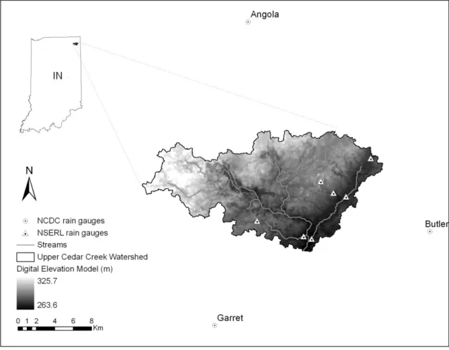
The study area for this work is the Upper Cedar Creek Watershed (UCCW) which is located 9

in the St. Joseph Watershed in northeastern Indiana (Fig. 1). The predominant landuse in the 10

UCCW is agricultural, with major crops of corn and soybeans, and minor crops of winter wheat, 11

oats, alfalfa, and pasture. The area receives approximately 94 cm of annual precipitation and 12

has average daily temperatures ranging from -1 °C to 28 °C. 13

The United States Department of Agriculture, Agricultural Research Service (USDA‐ARS) 14

National Soil Erosion Research Laboratory (NSERL) has established an environmental 15

monitoring network in UCCW as a part of the Source Water Protection Project and the 16

Conservation Effect Assessment Project. The environmental monitoring network in UCCW 17

has been operational since 2002. More details about the network can be found in Flanagan et 18

al. (2008). The UCCW environmental monitoring network provides considerable 19

meteorological data (10 minute rainfall, air temperature, solar radiation, wind speed and 20

relative humidity) and every 10 minute soil moisture observations at four different depths (5 21

20, 40 and 60 cm). Recently, UCCW has been selected as one of several USA core sites to be 22

used for calibration and validation of future SMAP data. Substantial in-situ data, and its 23

importance for future remote sensing validation work makes UCCW an ideal test bed for this 24

study. 25

In addition to the data from the monitoring network, daily precipitation and temperature data 26

are available from nearby three National Climatic Data Center (NCDC) weather stations for 27

the model simulation period, from 2003 to 2010. (Fig. 1). 28

For the SWAT simulation, sub-basins and stream network are delineated from the 30 meter 29

Digital Elevation Model (DEM) from the National Elevation Dataset. ArcSWAT, an ArcGIS 30

interface for SWAT, is used for delineating the sub-basins and creating other input files for the 1

model. By using a critical threshold area (CSA) of 500 ha, the UCCW is divided into 25 sub-2

basins. Further division of sub-basins into HRU units requires soil and land use information. 3

Soil information is retrieved from the Soil Survey Geographic Database (SSURGO) available 4

from the USDA Natural Resources Conservation Service. Major soil types in the UCCW and 5

their areas are summarized in Table 1. Landuse information is obtained from the 2001 National 6

Land Cover Data (NLCD 2001) produced by the Multi-resolution Land Characteristics 7

Consortium. The NLCD 2001 data for the UCCW is reclassified to 15 different landcover 8

classes for this study (Table 2). By using a 10% threshold for both landuse and soil, and 0% 9

threshold for slope, a total of 209 HRUs are generated for the UCCW using ArcSWAT. 10

3.2 Experiment setup 11

3.2.1 Synthetic experiment 12

Data assimilation study requires reliable observed data and decent knowledge on the 13

uncertainties in the model and observations. In the present study, a synthetic experiment is 14

performed to better understand how soil moisture data assimilation affects various hydrologic 15

processes in the watershed scale SWAT model. The synthetic experiment assumes that errors 16

in the model and observations are known, which allows us to focus only on the effect of data 17

assimilation. Thus, this synthetic experiment at watershed scale should contribute to the 18

practical application of the forthcoming remotely sensed soil moisture data. 19

In this study, it is assumed that surface soil moisture observation for each HRU is available 20

and the synthetic observed data is created by adding random observation errors with zero mean. 21

Considering that the typical microwave remote sensing data have a penetrating depth up to 5cm, 22

we also assume that the synthetically observed soil moisture is available for the top 5cm depth 23

and the input SSURGO soil database is modified so that each HRU has the first two layers in 24

the 5cm depth interval. 25

3.2.2 Scenarios setup 26

Our experiment includes three separate scenarios all run for the same time period: a true run, 27

open loop and the EnKF. First the experiment starts with the implementation of the “true” state 28

by running the model with all available rainfall data from the three NCDC stations and the 29

seven NSERL rain gauges (Fig. 1). To represent our imperfect knowledge of the true hydrologic 30

processes, the model is subsequently run with an intentionally poor set of initial conditions and 31

with “limited” forcing data from only NCDC rain gauges. Hereafter, this is called the “open 32

loop” scenario. The third scenario, referred to as “EnKF” includes model integration with all 1

the same input including rainfall and model parameters as the open loop, but updating soil 2

moisture by assimilating daily (synthetic) observed surface soil moisture through the EnKF. By 3

limiting precipitation input, which is the driving force of soil moisture and streamflow, while 4

keeping other model parameters unchanged, the EnKF scenario enables the determination of 5

the influence of the surface soil moisture assimilation on model predictions of profile soil water 6

content and other hydrological responses. 7

Conventionally, precipitation data measured at point rain gauges have been used for 8

hydrological modeling, despite its limitations in representing the spatial distribution and 9

variability of actual precipitation. In reality, many watersheds rely on the precipitation data 10

from the sparsely located rain gauges inside or around the watershed as our open loop scenario 11

represents. Therefore, in this study, we investigate how the surface soil moisture assimilation 12

may compensate for the errors from the inaccurate precipitation input by comparing the 13

aforementioned three scenarios (true, open loop and EnKF). 14

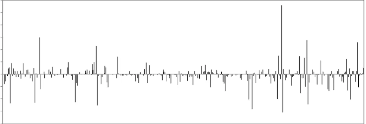
SWAT assigns precipitation values at the subbasin level based on precipitation data measured 15

at rain gauges. Each subbasin takes the precipitation value from the gage station that is closest 16

to the centroid of the subbasin. Unfortunately, there is no NCDC rain gauge inside the UCCW. 17

Therefore, when the precipitation data from the only three NCDC rain gauges are used (open 18

loop and EnKF), SWAT assigns overestimated precipitation into the watershed (Fig. 2). The 19

average precipitations of the true scenario and the open loop scenario (and EnKF) are 2.66 mm 20

day-1 and 3.21 mm day-1, respectively during the analysis period (from June 2008 to May 2009). 21

3.2.3 SWAT calibration 22

In order to create the true scenario, the SWAT model was calibrated using the daily 23

streamflow measured at the outlet of the UCCW. The model ran for three years (April 2003 to 24

April 2006) for warm-up and two years (May 2006 to May 2008) for calibration. Based on the 25

sensitivity analysis results, 18 parameters were chosen for calibration including CN2, ESCO, 26

SURLAG, TIMP, Ch_K2, SOL_AWC, BLAI, ALPHA_BF, SOL_Z, RCHRG_DP, SMTMP, 27

EPCO, CH_N2, REVAPMN, SLOPE, SOL_ALB, CANMX, SOL_K. They were calibrated 28

using the autocalibration tool, Parasol (Parameter Solutions) method, implemented in the 29

ArcSWAT. After the calibration, the model was validated for one year (June 2008 to May 2009). 30

The coefficient of determination (R2) and the Nash and Sutcliffe model efficiency coefficient 31

(ENS) are 0.46 and 0.44 for calibration period and 0.42 and 0.37 for validation period, 32

respectively with the daily streamflow predictions. Although these statistical metrics seem to 33

indicate marginal model performance, they are within an acceptable range at the daily time step 1

(Moriasi et al. 2007). This validation period will be used for our data assimilation experiment. 2

For the true scenario, the model runs from 2003 to 2009 with the calibrated parameters, and 3

the simulation results only from the last one year (June 2008 to May 2009) are used for analysis. 4

For the open loop and EnKF scenarios, the model runs from January 2008 to May 2009 with 5

an intentionally short warm-up period for poor initial conditions and the same calibrated 6

parameters as the true scenario. Again the last one year simulation results (June 2008 to May 7

2009) are used for analysis. 8

3.2.4 Evaluation metrics 9

Evaluation of the surface soil assimilation through the EnKF is first conducted by comparing 10

time series soil water storage and other representative hydrological responses obtained from 11

the true, open loop and EnKF scenarios. Root mean square error (RMSE), mean bias error 12

(MBE) and correlation coefficient (R) are used to compare the results quantitatively. 13















 





_

 





where T and S are true and simulated values respectively, and n is the number of data (days) 17

Tand Sare averages of true and simulated values respectively. 18

In addition, distributed soil moisture maps are shown to better visualize and illustrate the 19

spatial differences in the results and to determine the effect of spatially varying input. 20

3.3 Implementation of the EnKF into SWAT 21

3.3.1 Ensemble simulation with SWAT 22

The SWAT model runs on a daily time step. This study assumes that the daily soil moisture 23

observations are available, and therefore soil moisture condition is reinitialized for each day 24

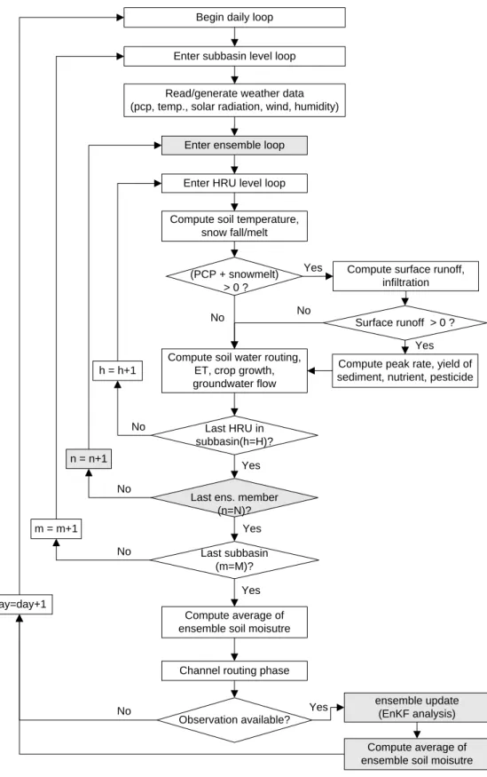
through the analysis (update) step of the EnKF. The framework of hydrologic processes in the 25

SWAT and additional routines due to the EnKF are illustrated in Fig. 3. The default SWAT 26

routines in Fig. 3 are excerpted from Neitsch et al. (2002). Each HRU runs independently and 27

one dimensional EnKF scheme is applied to each HRU separately. 28

Ensemble simulation starts on day 153 (June 1) of 2008 and 100 initial ensemble members 1

are created by adding random noise to the initial condition (soil moisture simulation results 2

from day 152). SWAT represents soil water content as a concept of soil water storage in 3

mmH2O (vs m3 m-3) and therefore the range of soil moisture values for each layer varies with 4

the thickness of the soil layer. The initial perturbation noise is assigned to the normalized soil 5

moisture values (mmH2O per 1cm). The initial perturbation noise has a Gaussian distribution 6

with zero mean and 0.001 mmH2O of standard deviation, and the magnitude of the standard 7

deviations are scaled by the thickness of each layer according to Ryu et al. (2009). Note that 8

forcing variables (e.g. precipitation) and model parameters are not perturbed explicitly to 9

generate ensemble members in this study. Adding model error (wk in the Eq. (5)) takes into

10

account all uncertainties raised from forcing variables and parameter estimation, as well as 11

model physics. 12

Each of the ensemble members of soil moisture goes through separate hydrological 13

processes and generates different subsequent variables such as Leaf Area Index and 14

evapotranspiration. All subsequent variables from different ensemble members are also 15

averaged after the ensemble forecasting step and the average values are considered as the best 16

estimations of the day. 17

3.3.2 Specification of model and observation errors 18

At the end of each day, the predicted ensemble soil moisture values are updated through the 19

EnKF analysis step. In the analysis step, model errors (wk in the Eq. (5)) with zero mean

20

Gaussian distribution are added. The standard deviations of the model errors are determined by 21

the current soil moisture content from the true scenario using a scaling factor of 0.01. 22

Observations are also perturbed with the observation errors (vk in the Eq. (9)) which have zero

23

mean Gaussian distribution and standard deviation of 0.01. 24

Procedures for soil moisture perturbation by adding system variance (model error) are 25

described as follows: 26

1) Compute a weight (wlj) for each layer (j) in order to take account for the different

27

thicknesses of each layer (Ryu et al., 2009). 28

2) Compute model noise (wk in the Eq. (5)) by applying a scaling factor (0.01) and a weight

29

(wlj) for each layer.

30





where θtrue,j is soil moisture estimation from the true scenario and rj is a random number from

a Gaussian distribution with zero mean and variance one for j=1,….,n where n is the number 1

of soil layers. 2

For soil moisture perturbation, a constant scaling factor is applied to all layers every daily 3

time step. Vertical correlation between perturbations is also an important factor in determining 4

how surface soil moisture assimilation affects deeper layers and other dependent variables. 5

Chen et al. (2011) showed the impact of error coupling with the SWAT model by comparing 6

the results from zero vertical error correlation and perfect vertical error correlation. In the 7

present study, perfect vertical error correlation was applied. 8

Several past studies have attempted to specify observation and model error statistics. Clark 9

et al. (2008) and Xie and Zhang (2010) used the scaling factor approach for straightforward 10

estimation of model and observation error. Reichle et al. (2002b) assigned temporally constant 11

standard deviations of errors. The scaling factor approach used in this study allows standard 12

deviation of the model errors to vary with time, which is a better representation of the real 13

uncertainties than the time invariant standard deviation of errors. Since our synthetic 14

experiment uses the same model parameters as the true scenario, the source of model error is 15

mainly from errors in the precipitation. Therefore, in this study, a simple but more operational 16

approach of using the scaling factor is adopted for model error estimation. This approach 17

overestimates the real errors when the soil moisture content is high, but is advantageous to test 18

the robustness of the EnKF (Xie and Zhang, 2010). The disadvantage of this approach, however, 19

is that it may enhance the nonlinear impact of the saturation (or wilting point) threshold by 20

inflating (or decreasing) the standard deviation of soil moisture predictions. In spite of 21

convenient application of the scaling factor approach, more sophisticated approaches such as 22

an adaptive filtering seem to be desirable for future real data assimilation studies. 23

Time invariant standard deviation of observation errors is adopted in this study because 24

errors in remotely sensed soil moisture come from vegetation cover, surface roughness, soil 25

properties, radio frequency interference (RFI), and retrieval algorithms, all of which are not 26

proportional to the surface soil moisture condition (Schmugge et al., 2002; Entekhabi et al., 27

2010). In addition, if the same scaling factor approach is applied to the observation error, it will 28

assign unreasonably high weight on the observation accuracy when the soil is very dry because 29

SWAT defines soil water content excluding the amount of water held at wilting point, with the 30

minimum soil water content in the SWAT being zero. 31

3.3.3 Additional steps in analysis procedure 32

The bounded nature of soil moisture between wilting point and saturated soil water content 33

makes the application of the EnKF more complicated. Reichle et al. (2002a) mentioned that in 1

an operational perspective, the violation of its inherent assumption, Gaussian distribution, 2

would have the greatest impact when the soil is very dry and there is high skewed forecast error. 3

Crow and Wood (2003) showed that the skewed model ensembles and a non-Gaussian error 4

structure negatively impacted the EnKF’s performances. Because of this unique characteristic 5

of soil moisture, some additional steps are added after the analysis step. When the soil is very 6

dry or wet (close to the wilting point or saturated condition), the best estimates of the soil 7

moisture (average of ensemble) after the analysis step may exceed the actual physical limits of 8

the soil moisture. If the average of the ensemble of the soil moisture becomes negative, the best 9

estimate of the ensemble is adjusted to 10 -6 mmH2O. In the case of an ensemble average higher 10

than the maximum soil moisture limit, saturated soil moisture content minus 10 -6 mmH2O 11

replaces the best estimate. 12

The concept of a simple bias correction method adopted by Ryu et al. (2009) is implemented 13

in this study to take account of the effect of the bounded range of soil moisture. Mean bias is 14

computed using the unperturbed soil moisture prediction and the ensemble is corrected by 15

subtracting the mean bias from the perturbed soil moisture ensemble. After this adjustment, all 16

ensemble members exceeding minimum or maximum soil water content are replaced by 10 -6 17

mmH2O (almost wilting point) or saturated water content. This boundary truncation might shift 18

the average of ensemble again. Therefore, these bias corrections and boundary truncations are 19

repeated 10 times to reduce the remaining bias. Boundary truncation and the simple bias 20

correction approach are applied at each update time step for all state variables (soil moisture 21

vector). A simple boundary truncation might cause the mean of the state variable to be shifted. 22

For example, for a wet soil moisture condition, the simple boundary truncation may shift the 23

mean of soil moisture higher than the actual mean from the analysis step. Therefore, this 24

repetition of boundary truncation and bias correction may be advantageous in generating less 25

mass balance error by decreasing the biases (Ryu et al. 2009). 26

4. Results and Discussion 27

4.1 Effect of surface soil moisture assimilation on hydrologic processes 28

This section describes how surface soil moisture data assimilation affects subsequent 29

hydrological processes. First, in this study, inaccurate precipitation is the main source of error 30

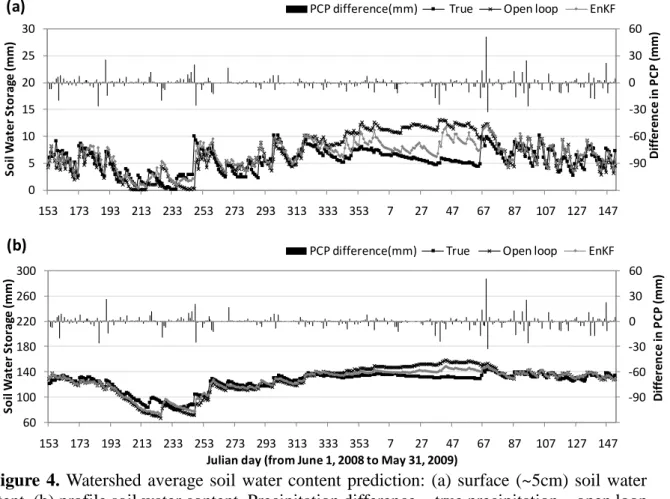
in soil moisture predictions as well as other hydrological processes. Fig. 4 shows the daily 31

simulation results of surface (a) and profile (b) soil moisture in the watershed which is the sum 32

of area-weighted soil water content from all HRUs. Soil moisture prediction errors are 1

significant especially during the winter time (from day 353 of the first year to day 67 of the 2

second year) due to the cumulatively overestimated precipitation shown in Fig. 2b. There exist 3

distinct discrepancies in soil moisture predictions between the true and the open loop scenario. 4

Soil moisture update through the EnKF draws the inaccurate soil moisture prediction in the 5

open loop scenario closer to the true state. The correlation coefficient increases from 0.585 to 6

0.747 and from 0.906 to 0.942 for surface and profile soil moisture respectively (Table 3). The 7

RMSE and MBE also decrease in both surface and profile soil moisture predictions with the 8

EnKF. The improved results with the EnKF support the previous studies (Das et al. 2008; 9

Draper et al. 2009; Reichle et al. 2002b; Sabater et al. 2007) further demonstrating the potential 10

of current and forthcoming remotely sensed surface soil moisture data to improve the profile 11

soil moisture estimations for land surface hydrology through data assimilation. The results of 12

this study also show that the errors in soil moisture estimation due to inaccurate precipitation 13

can be partially compensated by accommodating surface soil moisture observations. 14

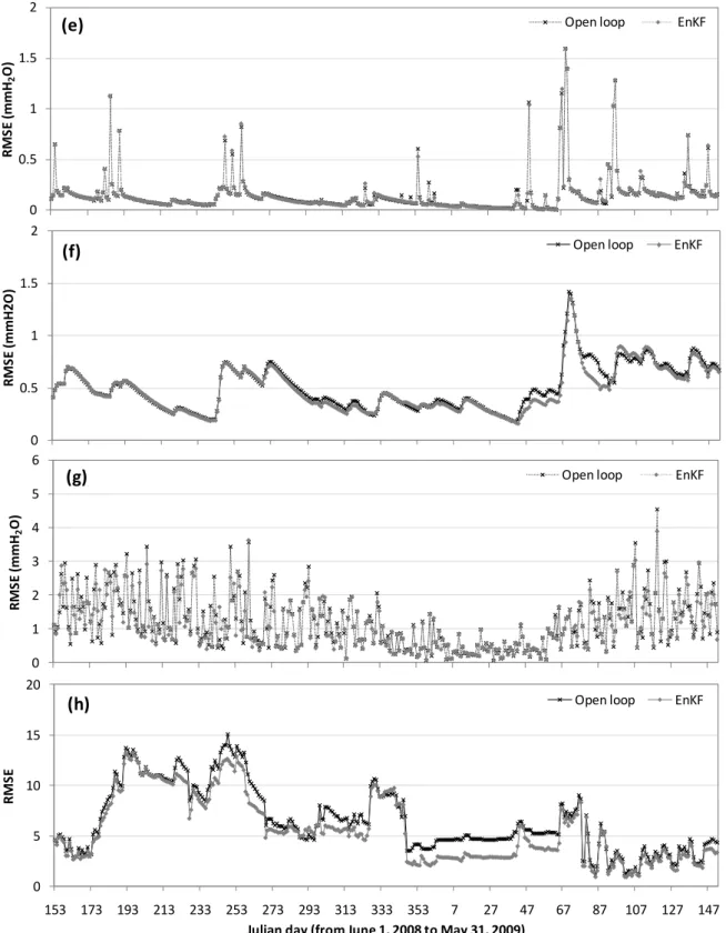
Temporal variations in the RMSE of the subsequent variables are shown in Fig. 5 where daily 15

RMSE is based on the errors of all HRUs. It is apparent that reduced errors in surface soil 16

moisture prediction (Fig. 5a) are clearly identified for almost every time step. In spite of the 17

prompt decrease of errors in surface soil moisture prediction, the magnitude of improvements 18

in the profile soil water content varies with time as shown in Fig. 5b with reduction in errors 19

with the EnKF being distinct in winter (from day 353 to 67). Limited success in updating profile 20

soil water content for some periods may be caused by the weak model vertical coupling of soil 21

moisture in SWAT subsurface physics (Chen et al., 2011). Another reason is that non-linearities 22

in model physics and the bounded nature of soil moisture result in suboptimal update with the 23

EnKF by violating the Gaussian assumption. When optimality of ensemble perturbation is 24

checked as in Reichle et al. (2002a), non-symmetric ensemble distribution is found with the 25

soil moisture condition close to saturation or wilting points (not shown). In addition, 26

consistently lower forecast and analysis error variances compared with actual error were found, 27

resulting in estimates less than optimal. 28

The improved soil moisture prediction affects other subsequent hydrological responses. Table 29

3 shows that the EnKF scenario reduces errors in other hydrological variables compared to the 30

open loop scenario even though the correlation coefficient for some variables may be slightly 31

lower (e.g., SHALLST, QDAY, RCHRG, GW_Q and GWSEEP). 32

Similar to the profile soil moisture in Fig. 5b, SHALLST (depth of water in shallow aquifer) 33

in Fig. 5c and GW_Q (groundwater contribution to streamflow) in Fig. 5f are not noticeably 1

affected except during winter conditions. Little differences in RMSE are observed in the 2

prediction of QDAY (surface runoff) in Fig. 5d and LATQ (lateral flow) in Fig. 5e. Since 3

accurate prediction of surface runoff (QDAY) and groundwater contribution (GW_Q) are 4

critical to streamflow prediction, it is expected from these results that surface soil moisture 5

assimilation may not improve streamflow prediction significantly. Further discussion of these 6

finding is provided in section 4.2. Application of EnKF reduced the RMSE in 7

evapotranspiration prediction throughout the experiment period (Fig. 5g). This is because 8

evaporation occurs mainly on the soil surface and the improved surface soil moisture condition 9

contributes to greater accuracy in simulating evaporation. Finally, the curve number for a day 10

(CNDAY) is computed based on the profile soil water content. Therefore, the trend of error 11

reduction in the curve number prediction (Fig. 5h) is very similar to the trend of the profile soil 12

moisture (Fig. 5b). 13

4.2 Streamflow prediction 14

The answer to the question “Can surface soil moisture data assimilation improve streamflow 15

prediction?” depends on the accuracy of precipitation input and antecedent soil moisture 16

condition. In order to answer to this question, four simple and different cases can be considered 17

accounting for only antecedent soil moisture conditions and the accuracy of precipitation data, 18

and assuming that the EnKF always improves soil moisture predictions close to the true values. 19

1) Model predicted antecedent soil moisture is less than the true soil moisture (θpredicted < θtrue

20

≈ θEnKF)and current precipitation is overestimated.

21

2) Model predicted antecedent soil moisture is greater than the true soil moisture (θpredicted >

22

θtrue≈ θEnKF)and current precipitation is overestimated.

23

3) Model predicted antecedent soil moisture is less than the true soil moisture (θpredicted < θtrue

24

≈ θEnKF) and current precipitation is underestimated.

25

4) Model predicted antecedent soil moisture is greater than the true soil moisture (θpredicted >

26

θtrue≈ θEnKF) and current precipitation is underestimated.

27

Cases 2 and 3 would provide improvement in streamflow prediction by updating soil 28

moisture through the EnKF. In Case 2, the overestimated antecedent soil moisture condition 29

will aggregate the error from the overestimated precipitation and therefore, updated (corrected 30

to lower) soil moisture with the EnKF will generate less error than the open loop. The same 31

principle can be applied to Case 3 where improved runoff prediction with the EnKF is expected 32

compared to the open loop. However, Cases 1 and 4 will generate more errors with the EnKF 1

than with the open loop. In Case 1, the underestimated antecedent soil moisture condition 2

counterbalances the error in the overestimated precipitation. Therefore, improved runoff 3

prediction occurs with the open loop rather than with the EnKF in this case. The same principle 4

is applied to Case 4. Therefore, a hypothesis, “Assimilating surface soil moisture observation 5

into a hydrologic model will improve streamflow (or surface runoff) prediction” is valid only 6

if we have accurate precipitation information. Crow and Ryu (2009) pointed out this limitation 7

of updating solely the antecedent soil moisture condition and designed an assimilation system 8

that simultaneously updates soil moisture and corrects rainfall input by taking into account soil 9

moisture observations. 10

Case 1 occurs in the results of this study during the summer, especially around day 259. The 11

EnKF improves soil moisture prediction (Fig. 4b and Fig. 5b). However, because of 12

inaccurately overestimated precipitation, improved soil moisture with the EnKF (higher soil 13

moisture prediction than the open loop results) results in overestimated runoff and streamflow 14

(Fig. 5d and Fig. 6). The lower model performance using the EnKF is primarily due to 15

inaccurate precipitation. Therefore, in this case, surface soil moisture assimilation does not 16

appear to improve streamflow prediction. 17

Results during winter time represent Case 2 where both soil moisture and precipitation are 18

overestimated. Application of the EnKF improves streamflow prediction during winter time 19

(Fig. 6, day 42 to 87). This is because the open loop continues overestimating soil moisture 20

during winter, but the EnKF improves the soil moisture prediction (lowers the overestimated 21

soil moisture in Fig. 4). Even though the improvement in runoff prediction (QDAY) due to the 22

improved soil moisture with the EnKF is not significant (Fig. 5d), the improved groundwater 23

contribution (GW_Q) also contributes to the improved (reduced) streamflow in Fig. 5f. 24

In this study, streamflow prediction does not show significant improvement even after 25

applying surface soil moisture assimilation. The primary reason for this is that most of the 26

errors in streamflow prediction are due to inaccurate precipitation input (Fig. 6, Fig. 7 and 27

Table 4). Second, SWAT model physics does not have sufficient vertical coupling strength to 28

constrain soil water content in deeper layers or in the root zone using the surface soil moisture 29

observations (Chen et al., 2011). Since surface runoff generation depends on profile soil water 30

content, failure to significantly improve estimates of profile soil water content impede 31

successful surface runoff (or streamflow) prediction. Therefore, improvement in streamflow 32

prediction is not expected when the improvement of profile soil water content with the EnKF 33

is of little or marginal consequence as shown in Fig. 5b. Lastly, the unsuccessful improvement 1

in streamflow prediction may be attributed to the limited sensitivity of surface runoff (or 2

streamflow) prediction to the change in soil moisture with the CN method implemented in 3

SWAT. Surface runoff is the main contributor to streamflow especially with high rainfall 4

intensity. Therefore, if the updated soil water content with the EnKF is not reflected properly 5

to the surface runoff estimation, improved streamflow prediction cannot be expected. 6

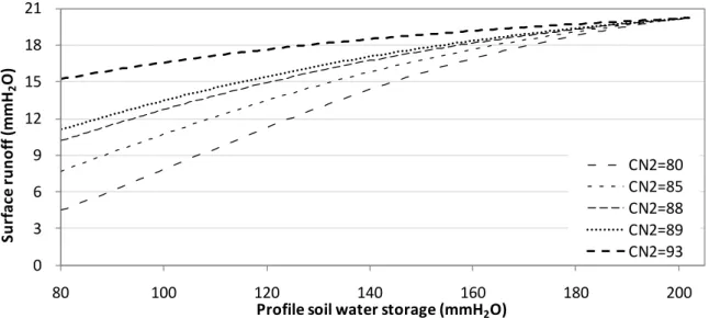
In order to test model sensitivity in these regards, the relationship between surface runoff 7

generation and different soil moisture conditions for various curve numbers is illustrated in Fig. 8

8 based on Eq. (2), (3) and (4). The soil type, GnB2, of which water storage at field capacity 9

and saturation are 101 mm and 201 mm respectively for a soil depth of 1246 mm, is used to 10

create Fig.8. In the case of high curve numbers (CN2=93), a 20 mm change in soil moisture 11

from 200 to 180 mm results in reducing surface runoff by only 2 mm. This decrease in runoff 12

prediction will result in a 4.57 m3 _sec-1 _{streamflow decrease, which is not sufficient to} 13

overcome the significant streamflow overestimation during the winter in Fig. 6. 14

As Fig. 8 shows, the sensitivity of surface runoff to soil water content varies with the curve 15

number, which is a function of soil type and landuse. This study also shows that the degree of 16

improvement in surface runoff prediction with the EnKF is highly related to soil type and 17

landuse. The areas which have low runoff error with the EnKF consist of soil types BoB, Hw, 18

SrB2, StC3 and Se (Table 1). Hydrologic soil groups of those soil types are A or B (Table 1). 19

Furthermore, the combinations of those soil types and landuse (HAY and FRSD) provide the 20

smallest errors because of their hydrologic soil group (A or B) and low CN2 (35 ~60). On the 21

contrary, the main three soil types (BaB2, GnB2 and Pe) which cover 67% of the area in the 22

UCCW produce high errors in surface runoff prediction regardless of landuse type. Their CN2 23

is relatively high (77 ~ 89). For most of the areas in UCCW the EnKF, therefore, cannot 24

decrease the error in the runoff prediction because surface runoff is not very sensitive to the 25

soil moisture change with high CN2 values. That is, the slope of the graph is small for high CN2 26

values in Fig. 8. Especially when soil moisture is high (close to saturation, 200mm in case of 27

GnB2), the slope is very small. During the winter time, highest soil moisture estimation errors 28

exist and the EnKF improves profile soil moisture up to 20 mm in Fig. 4b, but in this period, 29

the soil moisture condition is very wet, so its improvement is difficult to reflect in surface 30

runoff. 31

In this study, surface soil moisture assimilation was minimally successful in improving 32

streamflow predictions. However, if we consider only streamflow results, traditional 33

calibration methods can improve streamflow simulation considerably, even in the presence of 1

inaccurate precipitation. In SWAT, streamflow prediction has a higher sensitivity to changes in 2

certain parameters rather than changing soil moisture conditions. Parameter adjustments 3

through the calibration can change streamflow prediction effectively by increasing the ENS. 4

However, conventional calibration methods do not directly take into account the uncertainties 5

in precipitation or model structure, or the possibility of model parameters that change 6

temporally. Data assimilation techniques usually focus on updating state variables (soil 7

moisture in this study) on the premise that model parameters are pre-specified. Therefore, new 8

frameworks which can address both the limitations of conventional parameter calibrations and 9

data assimilation are required for future advances in hydrologic modeling. Moradkhani et al. 10

(2005), for example, showed the possibility of estimating both model states and parameters 11

simultaneously using a dual state-parameter estimation method based on the EnKF. 12

4.3 CN method vs. Green Ampt method 13

Even though the CN method has been widely used in various hydrologic models, it has 14

limitations. Garen and Moore (2005) stresses some issues with the broad use of the CN method. 15

Since the CN method was developed as an event model for the prediction of flood streamflow 16

conditions, they argue that it is questionable to apply the CN method for a continuous model 17

and daily flow of ordinary magnitude. In addition, they also mention that daily time step might 18

not be appropriate to simulate the infiltration excess mechanism which is designed for hourly 19

(or subhourly) time steps. 20

SWAT 2005 provides another option to estimate surface runoff, the Green Ampt Mein-21

Larson excess rainfall method (GAML). This method is based on the Green & Ampt infiltration 22

method and requires subdaily precipitation input. The CN method has been more widely used 23

than the GAML method because of the difficulties in obtaining subdaily precipitation data and 24

uncertain benefit of using the GAML compared to the CN method. While Kannan et al. (2007) 25

and King et al. (1999) found no significant advantages of using the GAML instead of the CN 26

method with SWAT, Jeong et al. (2010) showed that the GAML outperforms the CN method 27

and suggested that the quality of subdaily precipitation data and the size of study area influence 28

the results. In addition, Jeong et al. (2010) also showed that even the subhourly simulation 29

performs poorly under low or medium flows. 30

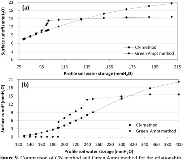
In this study, a simple experiment is conducted to test if the GAML method has a greater 31

potential than the CN method for improving runoff (and eventually streamflow) prediction with 32

surface soil moisture data assimilation. As mentioned in section 4.2, sensitivity of surface 1

runoff generation to the soil moisture change determines how successfully the soil moisture 2

update through the EnKF will contribute to the improvement of the surface runoff prediction. 3

For the two main soil types, GnB2 and SrB2, surface runoff was computed by using the CN 4

method and the GAML method for one day (June 21, 2008) when precipitation was 23mm day -5

1_{. For the GAML method, 10 minute precipitation data were used. The amount of water held} 6

in soil profile at field capacity is 101.5 and 240 mmH2O for GnB2 and SrB2, respectively. 7

Water content at saturation is 210 and 400 mmH2O for GnB2 and SrB2, respectively. 8

Fig. 9 shows the different runoff-soil moisture relationships from the CN and GAML 9

methods. The CN method maintains a smooth relationship between runoff and soil moisture, 10

however, the GAML method produces drastic changes when soil moisture is near field capacity 11

(101.5 and 240 mmH2O for GnB2 and SrB2 respectively). This is because the GAML code 12

implemented in SWAT2005 replaces any soil moisture value that is greater than field capacity 13

soil moisture with the field capacity value in computing infiltration rate. Therefore, under 14

higher soil moisture conditions, the GAML method produces much less surface runoff than CN 15

method, which is appropriate in reducing the overestimated streamflow. However, the slope of 16

the graph for GAML is much smaller than the slope of the CN method above field capacity. 17

Therefore, the impact of the improved soil moisture with the EnKF might be difficult to see 18

with the GAML method when the soil moisture is above field capacity. However, soil moisture 19

less than the field capacity has a high sensitivity to changes in soil moisture. The two different 20

soil types show different shapes of the relationship because of their different field capacity and 21

saturated water content values. Therefore, effectiveness of the soil moisture assimilation with 22

the GAML depends on the soil type and soil moisture condition. In using either the CN method 23

or GAML method, it is very difficult and somewhat complicated to determine precisely how 24

changes in soil moisture affect streamflow prediction. 25

Successful improvements of streamflow prediction through soil moisture data assimilation 26

can be expected only if the model is based on correct linkage between soil moisture conditions 27

and surface runoff generation. Even though SWAT 2005 adopts a modified CN method which 28

accounts for antecedent soil moisture condition continuously, its effectiveness is not thoroughly 29

proven. In addition, application of the CN method has been questioned by many studies and its 30

modification for runoff simulation has been introduced (Michel et al., 2005; Mishra and Singh, 31

2006; Chung et al., 2010; Sahu et al., 2010), specifically with SWAT (Kannan et al., 2008; Kim 32

and Lee, 2008; Wang et al., 2008; White et al., 2010). In addition, various factors such as 33

quality of rainfall data, rainfall intensity, soil type, landuse and identification of critical source 1

area make streamflow prediction more complicated. Therefore, more careful selection and 2

development of runoff simulation procedures effectively taking account for soil moisture 3

variations should be required to enhance streamflow prediction with future soil moisture 4

assimilation studies. 5

4. 4 Spatial variation in soil moisture prediction 6

In this section, the impact of spatially varying input, specifically landuse and soil type, on 7

surface soil moisture assimilation is illustrated. To visualize spatial distribution of output, an 8

HRU map is created by overlaying landuse and the SSURGO soil map generated from 9

ArcSWAT. Since a single slope is defined in the initial SWAT setup, the slope is not taken into 10

account in creating the HRU map. Then, HRU level outputs are assigned to each HRU to show 11

spatially distributed results. 12

Precipitation as a forcing variable is the most important factor for successful soil moisture 13

estimation. Fig. 10 shows time-averaged RMSE of precipitation. Time-averaged RMSE results 14

of surface and profile soil moisture prediction are shown in Fig. 11 and 12 respectively. The 15

RMSE distribution of the open loop and the EnKF, especially for profile soil moisture 16

distribution, coincides with the distribution of precipitation in general. That is to say, higher 17

precipitation errors within an area result in greater errors in soil moisture estimation. 18

The EnKF reduces errors in surface and profile soil moisture compared to the results of the 19

open loop. The average RMSE errors in surface soil moisture estimates in Fig. 11 are 5.05 and 20

3.43 mmH2O for the open loop and the EnKF, respectively. For profile soil moisture estimation, 21

the open loop and the EnKF have 22.77 and 19.77 mmH2O of average RMSE, respectively in 22

the Fig. 12. 23

Within a subbasin where constant precipitation is assigned, types of landuse and soil determine 24

the magnitude of errors in the soil moisture estimation. One distinct example is shown in 25

subbasin 2 in Fig. 11a. Even though the subbasin has same amount of precipitation throughout 26

the area, some of the areas (light blue in the Fig. 11a) have highly underestimated surface soil 27

moisture (much higher RMSE) than others. The areas consist of HRU 11(FRSD, Hw), 28

18(AGRR, Hw) and 21(WETF, GnB2). The soil type Hw is classified as hydrologic soil group 29

A (Table 1) which has a high infiltration rate. 30

Fig. 13 compares the results of different combinations of landuse and soil types. Fig. 13b is 31

the reference because it consists of the major landuse (AGRR) and soil type (GnB2). 32

Comparing Fig. 13b and 13c explains the effect of different soil types on soil moisture 1

estimation. Although landuse type and precipitation are same, Fig. 13c which has more 2

infiltration rate because of the soil type Hw, exaggerates both the underestimated and 3

overestimated errors compared to the soil type GnB2 in Fig. 13b. 4

Types of landuse also affect the soil moisture variations. Fig. 13a and 13d show that landuse 5

types, forest (FRSD) and wetland (WETF), produce greater errors than agricultural area. 6

Proportion of precipitation intercepted by canopy is large in forest area. Therefore, the actual 7

precipitation that reaches the ground (after canopy interception) in this area may be much 8

smaller than other landuse areas, which will exaggerate errors in soil moisture estimation. 9

Further explanation regarding the errors due to different landuse types follows in section 4.5. 10

4.5 Spatiotemporal variation in soil moisture prediction 11

Aforementioned results show significant effects of errors in precipitation on hydrologic 12

responses. In this section, the effect of precipitation is excluded by selecting a drydown period 13

when no precipitation is received throughout the watershed. Therefore, the effectiveness of the 14

EnKF can be further evaluated. 15

Fig. 14c and 14d show the antecedent surface soil moisture condition in terms of deviations 16

(errors) from the true condition on day 258 before the precipitation events on day 259 shown 17

in Fig. 14a and 14b. The western areas of the UCCW have overestimated soil moisture 18

(negative error) and eastern areas have underestimated states (positive error) on day 258. On 19

day 259 in Fig. 14e and 14f, highly overestimated precipitation in subbasins 1, 3, 4, 5, 6 and 7 20

do not make much differences in soil moisture status because soil moisture is already 21

overestimated (close to saturated condition) and the overestimated precipitation becomes 22

surface runoff instead of infiltrating into the soil and increasing soil moisture. However, 23

slightly overestimated precipitation in subbasins 2, 8, 14, 15, 18, 19, 20, 21 and 24 infiltrates 24

into soil and decreases the errors in the previously underestimated soil moisture. 25

After the precipitation on day 259, there is no precipitation at all throughout the watershed 26

until day 263. While errors in surface soil moisture estimation in the open loop do not change 27

significantly day by day, the EnKF results show noticeably decreasing errors in one or two 28

days. In other words, errors in the EnKF results become close to zero sooner than the open loop 29

results. In regard to the profile soil moisture variations, the EnKF produces better results 30

(smaller errors in general) than the open loop results even though the magnitudes of 31

improvements are not as much as the ones with the surface soil moisture (not shown). 32