Abstract— In this paper, the free vibration characteristics of
an elastically connected non-prismatic double-beam system based on Euler-Bernoulli beam theory are determined using differential transform method. The double-beam system is composed of two parallel non-uniform cantilever beams which are attached to each other by a Pasternak elastic medium. Numerical results of the method used are validated by comparing with the ones available in the published literature. The effect of the taper ratio on the natural frequency of the double-beam system is also studied.
Index Terms— double-beam system, non-prismatic beam,
Pasternak elastic layer, taper ratio, cantilever beam
I. INTRODUCTION
REE and forced vibrations of single beams with uniform and non-uniform cross-section have been studied by several researchers because of their useful applications in many fields of engineering. These are reported in [1]-[14].
An important extension of the concept of the single beam is that of the multiple or compound beam system, for instance, double-beam system, triple-beam system and so on. The vibration problem of beam-type structures such as elastically connected double-beam system is still a subject of great interest to investigators. The physical model of a double-beam system is usually composed of two parallel beams, prismatic (or non-prismatic) coupled together by innumerable coupling springs ([14],[16]).
The vibration problem of two beams which are elastically connected is of great interest to practitioners in many fields of engineering. To this end, different cases of the vibration of elastically connected double-beam systems have been attempted by several scholars. Seelig and Hoppmann II [17] presented the frequencies and associated mode shapes of a system of n elastically connected parallel beams having different support conditions. They used the result obtained for the general n-system to give detail analysis of the particular case of a two-beam system. As reported in [17],
Manuscript received February 19, 2017; revised March 13, 2017. This work was supported fully by Covenant University, Ota, Nigeria.
O. O. Agboola is with the Department of Mathematics, Covenant University, Ota, Nigeria (+2348032502412; e-mail: ola.agboola@ covenantuniversity.edu.ng).
J. A. Gbadeyan is with the Department of Mathematics, University of Ilorin, Ilorin, Nigeria. (e-mail: [email protected]).
S. A. Iyase is also with the Department of Mathematics, Covenant University, Ota, Nigeria (e-mail: [email protected]).
application of beam theory to the vibration of double-beam systems which are elastically coupled has been earlier studied by Dublin and Friedrich (1956) and Osborne (1962). Oniszczuk [18] developed the free transverse theory of an elastically connected simply supported double-beam system continuously joined by a Winkler elastic layer. The motion of the system was solved using the Bernoulli-Fourier method. Gbadeyan and Agboola [19] investigated dynamic behaviour of visco-elastically connected uniform double-beam system carrying uniform partially distributed moving load based on Euler-Bernoulli theory. Abu-Hilal [14] investigated the dynamic response of a simply supported double-beam system subjected to a constant moving load.
Mao [20] employed Adomian decomposition method to study the free vibrations of elastically connected beams under general conditions. The system considered is composed of uniform Euler-Bernoulli beams which are continuously joined by a Winkler-type elastic layer. Huang and Liu [21] investigated the free and forced vibration analyses of two parallel prismatic beams connected to each other by uniformly distributed vertical springs. The inner springs are also stimulated Winkler model. Using finite element method for the analysis, it is found that the inner spring with large coefficient has significant effect on the natural frequencies of out-of-phase vibration. Li, Hu and Sun [22] used a semi-analytical method to obtain the natural frequencies and corresponding mode shapes of a double-beam system interconnected by a viscoelastic layer of the Winkler type. They further studied the effects of viscoelastic layer damping and Winkler layer on the vibration characteristics of the double-beam system.
Virtually, all the above research works assumed that the two beams that make up the double-beam system are prismatic having uniform cross-section. It has also been observed from the above literature that no research work has been done to investigate the free vibration analysis of a system of two non-prismatic beams coupled by a Pasternak elastic layer. Thus, in this article, the differential transform method is further developed to analyse the free vibration of a non-prismatic double-beam system connected by a Pasternak elastic layer under clamped-free boundary conditions and based on Euler-Bernoulli beam theory.
II. GOVERNING EQUATIONS OF MOTION
The equations of motion governing the free vibration of a
Vibration of an Elastically Connected
Non-prismatic Double-beam System Using
Differential Transform Method
Olasunmbo O. Agboola, Member, IAENG, Jacob A. Gbadeyan, and Samuel A. Iyase
non-prismatic double-beam system elastically connected by a Pasternak layer are given by:
2 2
2
1 1
1 1 1 1
2 2 2
2
1 2 2
, ,
( ) ( ) , , 0
w x t w x t
E I x A x
x x t
k x G x w x t w x t
x
, (1)
and
2 2
2
2 2
2 2 2 2
2 2 2
2
2 1
, ,
( ) ( ) , , 0
w x t w x t
E I x A x
x x t
k x G x w x t w x t
x
, (2)
where wj
x t, is the transverse displacement of the jth beam at any distance x along the length of the beam at timet. The subscriptj is associated with the upper beam (j = 1) and lower beam (j =2). Aj
x and Ij
x are the area of cross-section and cross-sectional moment of inertia of jth at distance x from the left end of the jth beam respectively.j
E and j are the Young’s modulus of elasticity and mass density of the jth beam material respectively. k x
is the variable Winkler modulus of the elastic layer (springs) that joins the two beams and G x
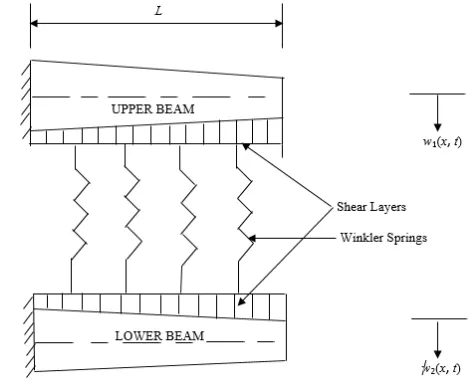
is the variable shear modulus that accounts for the shear interaction among the springs.The boundary conditions considered at the ends of the each of the beams (being cantilever), as shown in Fig. 1, can be expressed as
0, 0, j
0, 0; 1, 2y
dw t
w t j
dx
(3)
at the fixed end, and
2 3
2 3
, ,
0, 0; 1, 2
j j
d w L t d w L t
j
dx dx (4) at the free end.
For Eqs. (1) and (2), we assume a solution of the form: ( , ) ( ) i t, 1, 2
j j
w x t Y x e j (5)
whereYj
x is the mode shape of the jth beam and the angular frequency of the system.By using Eq. (5) in Eqs. (1) and (2), the equations of motion reduce to
2 2
1 2
1 1 1 1 1
2 2
2
1 2 2 1 2
( ) ( ) 0
d Y x d
E I x A x Y x
dx dx
d
k x Y x Y x G x Y x Y x
dx
[image:2.612.304.542.50.245.2], (6)
Fig. 1. The structural model of a system of two non-prismatic beams elastically connected with a Pasternak elastic layer
and
2 2
2 2
2 2 2 2 2
2 2
2
2 1 2 2 1
( ) ( ) 0
d Y x d
E I x A x Y x
dx dx
d
k x Y x Y x G x Y x Y x
dx
.
(7)Similarly, Eqs. (3) and (4) imply that
0, j
0; 1, 2j
dY x
Y x j
dx
,
(8) and
2 3
2 0, 3 0; 1, 2
j j
d Y x d Y x
j
dx dx
.
(9) For simplicity, the following non-dimensional parameters are introduced:
( ) ( )
, ( ) , , ( )
(0) (0)
j j j
j j j
j j
Y x I x A x
x
y I A
L L I A
.(10)
Thus, Eqs. (6) and (7) can be written as
2 2
2 2 1
1 1 1 1
2 2
2
1 1 2 1 2 1 2
d ( ) d
( )
d d
d
( ) ( ) ( ) ( ) ( ) ( ) 0
d y
I A y
y y G y y
, (11)
2 2 2 2 22 2 2 2
2 2
2
2 2 1 2 2 2 1
d ( ) d
( )
d d
d
( ) ( ) ( ) ( ) ( ) ( ) 0
d y
I A y
y y G y y
(12) such that
4 4 2 1 1 2 1 1 0 ( ) ( ) ( ) , , ( )(0) 0 0
j j j
j j j j
A L
k x L G x L
G
E I E I E I
(13)
Also, the boundary conditions in Eqs. (8) and (9) can be written in the following non-dimensional form:
0, j
0; 1, 2 j dy y j d (14)
at 0, and
2 3
2 0, 3 0; 1, 2
j j
d y d y
j
d d
(15)
at 1.
III. DTM ALGORITHM AND SOLUTION PROCEDURES A. DTM Algorithm
The differential transform method (DTM) is briefly described herein for completeness consideration. In DTM, the function ( )y and its rth order derivative with respect to are approximated via a differential transform as:
0 ( ) 1 ( ) ! r r d y Y r
r d
(16)
The inverse differential transformation of convolution ( )
Y r is defined as
0
( ) r ( )
r
y Y r
. (17)Combining equations Eqs. (16) and (17), we have
0 0 ( ) ( ) ! r r r r d y y
r d
.
(18)The basic operations of the dimensional transform which are useful in the transformation of the governing equations and the boundary conditions are summarized as follows: [23],[25],[29]
Original function Transformed function ( ) ( ) ( )
f g h
F r( )G r( )H r( )
( ) ( )
f g
F r( )G r( )
( ) ( ) ( )
f g h
0
( ) ( ) ( ); /
r
r
F r G s H r s
( ) ( ) n n d g f dx ( ) ( )! ( ) ! r nF r G r n
r
( ) n
f
( ) ( ) 1 if
0 if r n
F r r n
r n
B. Solution by DTM
By applying the DTM operations appropriately, the differential transform of Eqs. (11) and (12) are obtained as 1 1 0 1 0 1 1 0 1 2 2 1
1 1 1 1 2
0 0
1 1 2
0
1 2 3 4 4
2 1 1 1 2
3 3
1 2 2 1
2 2
( )
( )( 1)( 2) 2 2 0
r s r s r s r r s s r s
I r s s s s s Y s
r s I r s s s
s Y s
r s r s I r s s
s Y s
A r s Y s r s Y s Y s
G r s s s Y s Y s
,
(19)and 2 2 0 2 2 0 2 2 0 2 2 2 2
2 2 2 1
0 0
2 2 1
0
1 2 3 4 4
2 1 1 1 2 3 3
1 2 2 1 2 2
( )
( )( 1)( 2) 2 2 0
r s r s r s r r s s r s
I r s s s s s Y s
r s I r s s s s Y s
r s r s I r s s s Y s
A r s Y s r s Y s Y s
G r s s s Y s Y s
. (20)
The following transformed boundary conditions are also obtained:
(0) 0, (1) 0 1, 2
j j
Y Y j , (21) and
0 0
( 1) ( ) 0, ( 1)( 2) ( ) 0
M M
j j
r r
r r Y r r r r Y r
. (22)We then solve Eqs. (19) and (20) subject to Eqs. (21) and (22) for the natural frequency, by re-arranging the set of algebraic equations to obtain an eigenvalue problem.
1(2) , 1(3) , 2(2) , 2(3)
Y a Y b Y c Y d (23) The values of Y1(4),Y1(5),,Y M1( ) and
2(4), 2(5), 2( )
Y Y Y M can be determined in terms , , ,a b c dby using Eqs. (21) appropriately in Eqs. (19) and (20) setting
0,1, 2,
r . Next, Yj(0), Yj(1), Yj(2),…, Yj(M) for 1, 2
j are substituted into Eqs. (22) which yield a system of four equations in corresponding to the Mthterm. The system of equations can be written in the matrix form
( ) ( ) ( ) ( ) 1 11 12 13 14
( ) ( ) ( ) ( ) 2 21 22 23 24
( ) ( ) ( ) ( ) 3 31 32 33 34
( ) ( ) ( ) ( ) 4 41 42 43 44
0
( ) ( ) ( ) ( )
0
( ) ( ) ( ) ( )
0
( ) ( ) ( ) ( )
0
( ) ( ) ( ) ( )
M M M M
M M M M
M M M M
M M M M
c
f f f f
c
f f f f
c
f f f f
c
f f f f
. (24)
It should be noted that Eqs. (24) has a non-trivial solution provided the determinant of the coefficient matrix is zero. That is,
( ) ( ) ( ) ( ) 11 12 13 14
( ) ( ) ( ) ( ) 21 22 23 24
( ) ( ) ( ) ( ) 31 32 33 34
( ) ( ) ( ) ( ) 41 42 43 44
( ) ( ) ( ) ( )
( ) ( ) ( ) ( )
0
( ) ( ) ( ) ( )
( ) ( ) ( ) ( )
M M M M
M M M M
M M M M
M M M M
f f f f
f f f f
f f f f
f f f f
. (25)
Solving the characteristic Eq. (25) yields the natural frequency of the double-beam system. One obtains
( )
, 1, 2, M
n n
as the Mth estimated natural frequency corresponding to nth mode of vibration. The value of M is decided by the convergence of natural frequency expressed by the inequality:
( ) ( 1)
,
M M
m m
where is the error tolerance parameter taken as 0.0001 in this paper.
IV. NUMERICAL EXAMPLE
To illustrate the theory presented, the vibration characteristics of a beam pair with constant width and linearly varying height are studied in this section. To this end, the area of cross-section and the moment of inertia of the jth beam vary per the following relations:
( ) (0) 1 ; 1, 2
j j j
x
A x A j
L
, (26)
and
3
( ) (0) 1 ; 1, 2
j j j
x
I x I j
L
, (27)
where Aj(0) and Ij(0) are the area of the cross-section and
moment of inertia at the left end of the jth beam, j is the taper ratio for jth beam which satisfies 0j 1.
Writing Eqs. (26) and (27) in non-dimensional form one gets
j( ) 1 j , 1, 2
A j , (28) and
3j( ) 1 j , 1, 2
I j . (29) For validation, the values of the parameters which describe the material and geometrical properties of the uniform Euler-Bernoulli double-beam system from the work of Mao [20] is used in our analysis. In this case, the length of each beam is L = 10 m, while the material and geometric properties of the upper beam are:
10 1 1 10
E 2
Nm ,
2 1(0) 1 5 10
A A m2,
4 1(0) 1 4 10
I I m4, 3 1 2 10
kgm-3.
For the lower beam, the flexural stiffness and the mass per unit length are: E I2 2 2 E I1 1 and 2A2 2 1A1
respectively. The Winkler modulus of the inner springs used for the computation is 5
1 10
k Nm-2. By using these
values, the natural frequencies are calculated and the results are shown in Table I. The results reported by Mao [20] using Adomian Modified Decomposition method (AMDM) are based on a uniform double-beam system elastically connected by a Winkler layer are compared with the ones obtained using DTM by neglecting the Shear modulus parameter (G x
0).TABLEI
COMPARISON OF THE FIRST SIX NATRURAL FREQUENCIES BY METHODS FOR CANTILEVER PRISMATIC EULER-BERNOULLI (EB) DOUBLE BEAM SYSTEM COMPOSED OF NON-IDENTICAL
BEAMS AND JOINED BY WINKLER ELASTIC LAYER
Frequency AMDM, Mao [20] Present
1
7.0320 7.0320
2
39.3630 39.3629
3
44.0690 44.0690
4
58.6692 58.6709
5
123.3944 123.3944
6
129.3297 129.3324
The results in Table I show that there is a close agreement between DTM and AMDM, hence validating the present study
The effects of taper ratio on the first four natural frequencies of a double-beam system composed of two non-identical Euler-Bernoulli (EB) beams connected by a Pasternak elastic medium are displayed in Table 2 for clamped-free boundary conditions. The physical properties of the beams used for the calculations are:
10 1 1 10
E 2
Nm , A1(0) A1 5 102
4 1(0) 1 4 10
I I m4, 3 1 2 10
kgm-3.
The flexural stiffness and the mass per unit length of the lower beam are: E I2 2 2 E I1 1 and 2A2 2 1A1
respectively. The values of the moduli of Winkler layer and shear layer used are 5
2 10
k Nm-2 and G100Nm-2,
respectively. Constant moduli of the layer are assumed.
TABLEII
THE FIRST FIVE NATURAL FREQUENCIES OF NON-PRISMATIC CANTILEVER DOUBLE-BEAM SYSTEM ELASTICALLY CONNECTED BY A PASTERNAK LAYER FOR DIFFERENT VALUES
OF TAPER RATIO (NON-IDENTICAL CASE)
Frequency 0 0.25 0.50
1
7.0320 7.2725 7.6476
2
44.0690 40.5078 36.6345
3
55.2217 61.6178 69.3677
4
70.3013 72.2055 78.3339
5
123.3944 109.5368 94.5297
6
135.0069 124.4988 115.4559
We observed that increasing the taper ratio resulted in increase in the natural frequency of the double-beam system under consideration for the first four modes of vibration. Contrarily, we noticed that there was a decrease in the fourth and fifth natural frequencies of the system due to increase in the taper ratio.
V. CONCLUSION
In this paper, the free vibrations of a system of two non-prismatic cantilever beams elastically attached by a Pasternak layer and based on Euler-Bernoulli beam theory are considered. The results obtained using a semi-analytical approach known as differential transform method (DTM) were validated against those earlier reported in the literature. Also, the effects of the taper ratio on the natural frequencies of the double-beam system were discussed.
REFERENCES
[1] K. R Chun, “Free vibration of a beam with one end spring–hinged and the other free,” Journal of Applied Mechanics, vol. 39 no. 4, pp. 1154–1155, 1972.
[2] D. A. Grant, “Vibration frequencies for a uniform beam with one end elastically supported and carrying a mass at the other end,” Journal of Applied Mechanics, vol. 42, pp. 878-880, 1975.
[3] M. J. Maurizi, R. E Rossi, and J. A. Reyes, “Vibration frequencies for a uniform beam with one end spring–hinged and subjected to a translational restraint at the other end,” Journal of Sound and Vibration, vol. 48, pp. 565–568, 1976.
[4] T. R. Hamada, “Dynamic analysis of a beam under a moving force: A double Laplace transform solution,” Journal of Sound and Vibration, vol. 74 no. 2, pp. 221–233, 1981.
[5] E. Esmailzadeh and E. Ghorashi, “Vibration analysis of beams traversed by uniform partially distributed moving masses,” Journal of Sound and Vibration, vol. 184, pp. 9–17, 1995.
[6] J. T.–S. Wang and C.–C. Lin, “Dynamic analysis of generally supported beams using Fourier series,” Journal of Sound and Vibration, vol. 196, no. 3, pp. 285–293, 1996.
[7] R.–F. Fung and C.–C. Chen, “Free and forced vibration of a cantilever beam contacting with a rigid cylindrical foundation,” Journal of Sound and Vibration, vol. 202, pp. 161–185, 1997.
[8] N. M Auciello, and M. J. Maurizi, “On the natural vibrations of tapered beams with attached inertia elements,” Journal of Sound and Vibration, vol. 199, no. 3, pp. 522–530, 1997.
[9] W. Yeih, J. T. Chen, and C. M. Chang, “Applications of dual MRM for determining the natural frequencies and natural modes of an Euler–Bernoulli beam using the singular value decomposition method,” Engineering Analysis with Boundary Elements, vol. 23, no. 4, pp. 339–360, 1999.
[10] J. A. Gbadeyan, and S. T. Oni, “Dynamic behavior of beams and rectangular plates under moving loads,” Journal of Sound and Vibration, vol. 182, pp. 677-695, 1994.
[11] M. A Foda, and Z. Abduljabbar, “A dynamic Green function formulation for the response of a beam structure to a moving mass,” Journal of Sound and Vibration, vol. 210, pp. 295–306, 1998. [12] J–J Wu, A. R. Whittaker, and M. P. Cartmell, “Dynamic responses of
structures to moving bodies using combined finite element and analytical methods,” International Journal of Mechanical Sciences, vol. 43, no. 11, pp. 2555–2579, 2001.
[13] S. Naguleswaran, “Transverse vibration of an uniform Euler– Bernoulli beam under linearly varying axial force,” Journal of Sound and Vibration, vol. 275, pp. 47–57, 2004.
[14] M. Abu–Hilal, “Dynamic response of a double Euler–Bernoulli beam due to a moving constant load,” Journal of Sound and Vibration, vol. 297, no. 3-5, pp. 477–491, 2006.
[15] I. Zamorska, “Free transverse vibrations of non–uniform beams,” Scientific Research of the Institute of Mathematics and Computer Science, vol. 9, no. 2, pp. 243–249, 2010.
[16] J. Li, and H. Hua, “Spectral finite element analysis of elastically connected double–beam systems,” Finite Elements in Analysis and Design, vol. 43, pp. 1155–1168, 2007.
[17] J. M. Seelig, and W. H. Hoppmann II, “Normal mode vibrations of systems of elastically connected parallel bars,” Journal of the Acoustical Society of America, vol. 36, pp. 93–99, 1964.
[18] Z. Oniszczuk, “Free transverse vibrations of elastically connected simply supported double-beam complex system,” Journal of Sound and Vibration, vol. 232, no. 2, pp. 287–403, 2000.
[19] J. A. Gbadeyan, and O. O. Agboola, “Dynamic Behaviour of a double Rayleigh beam-system due to uniform partially
distributed moving load,” Journal of Applied Sciences Research, vol. 8, no. 1, pp. 571-581, 2012.
[20] Q. Mao, “Free vibration analysis of elastically connected multiple-beams by using the Adomian modified decomposition method,” Journal of Sound and Vibration, vol. 331, pp. 232–2542, 2012. [21] M. Huang, and J. K. Liu, “Structural method for vibration analysis of
the elastically connected double-beam system,” Advances in Structural Engineering, vol. 16, pp. 365–377, 2013.
[22] Y. X. Li, Z. J. Hu, and L. Z. Sun, “Dynamical behavior of a double-beam system interconnected by a viscoelastic layer,” International Journal of Mechanical Sciences, vol. 105, pp. 291–303, 2016. [23] A. Mirzabeigy, “Semi-analytical approach for free vibration analysis
of variable cross-section beams resting on elastic foundation and under axial force,” International Journal of Engineering, vol. 27, no. 3, pp. 385-394, March 2014.
[24] T. Aida, S. Toda, N. Ogawa, and Y. Imada, “Vibration control of beams by beam-type dynamic vibration absorbers,” Journal of Engineering Mechanics, vol. 2, pp. 248-258, 1992.
[25] A. Arikoglu, and I. Ozkol “Solution of boundary value problems for integro–differential equations by using differential transform method,” Applied Mathematics and Computation, vol. 168, no. 2, pp. 1145–1158, 2005.
[26] S. H. Ho, and C. K. Chen, “Analysis of general elastically end restrained non–uniform beams using differential transform,” Applied Mathematical Modelling, vol. 22, pp. 219–234, 1998.
[27] B. Mehri, A. Davar, and O. Rahmani, “Dynamic Green function solution of beams under a moving load with different boundary conditions,” Transaction B: Mechanical Engineering, vol. 16, no. 3, pp. 273-279, 2009.
[28] S. Motaghian, M. Mofid, and P. Alanjari, “Exact solution to free vibration of beams partially supported by an elastic foundation,” Scientia Iranica, vol. 18, no. 4, pp. 861-866, 2011.