CIRJE Discussion Papers can be downloaded without charge from: http://www.e.u-tokyo.ac.jp/cirje/research/03research02dp.html
Discussion Papers are a series of manuscripts in their draft form. They are not intended for circulation or distribution except as indicated by the author. For that reason Discussion Papers may not be reproduced or distributed without the written consent of the author.
CIRJE-F-481
Efficient Gibbs Sampler for
Bayesian Analysis of a Sample Selection Model
Yasuhiro Omori University of Tokyo
Efficient Gibbs sampler for
Bayesian analysis of a sample selection model
Yasuhiro Omori
Faculty of Economics, University of Tokyo, Tokyo 113-0033, Japan
February 2007, revised March 2007
Abstract
We consider Bayesian estimation of a sample selection model and propose a highly efficient Gibbs sampler using the additional scale transformation step to speed up the convergence to the posterior distribution. Numerical examples are given to show the efficiency of our proposed sampler.
Key words: Bayesian analysis, Gibbs sampler, Sample selection model, Tobit model.
1
Introduction
A sample selection model or generalized Tobit (Type II Tobit) model has been very popular in the econometric analysis of the labour supply and wage function. It has been well-known as a generalization of the standard Tobit (Type I Tobit) model in econometrics since it was first introduced by Tobin (1958) to analyze the relationship between household income and household expenditures on a durable good where there are some households with zero expenditures (see e.g. Amemiya (1984) for a survey). Bayesian estimation method of a standard Tobit model using Monte Carlo method was proposed by Chib (1992). Chib (1992) developed Gibbs sampling procedure using the idea of data augmentation, which is widely used in the literature, and compared the efficacy of several Monte Carlo methods.
This article develops a related approach for a sample selection model and show that the con-vergence to the posterior distribution can be greatly accelerated by adding one or more sampling steps to the benchmark Gibbs sampler. Numerical examples suggest that the benchmark samplers suffer from inefficiencies and produces highly autocorrelated samples. The additional Gibbs move recovers efficiencies and reduces the sample autocorrelations dramatically. The rest of the paper is organised as follows. In Section 2, we introduce a sample selection model and describe benchmark Gibbs samplers. Section 3 proposes an additional sampling step to accelerate the convergence to the posterior distribution. Numerical examples are given in Section 4.
2
Bayesian analysis of a sample selection model
In a sample selection model, the sample rule is determined by a latent random variable z∗
i,and we
observe the response variable yi when zi∗ ≥ 0. The latent variable zi∗ is allowed to be correlated
with the response variable y∗
i.When the correlation coefficient,ρ, between (zi∗, yi∗) is not equal to
zero, a sample selection model is considered a Type I Tobit (a censored regression) model with a stochastic threshold model.
The sample selection model or a generalized Tobit (Type II Tobit) model for thei-th individual is given by yi = ( y∗ i, ifzi∗ ≥0, n.a., otherwise, i= 1,2, . . . , n, z∗i = w′iθ+ξi, yi∗ =x′iβ+ηi, (ξi, ηi)′ ∼i.i.d. N(0,Σ), (1)
where yi is a dependent variable, y∗i, zi∗ are latent dependent variables, (wi,xi) are independent
variable vectors, and (θ,β) are corresponding coefficient vectors. The disturbance vector (ξi, ηi)′
follows a bivariate normal distribution with mean0and covariance matrix Σ.The (1,1) element of
Σ is set equal to 1 for the identification and we use the following parameterisation as in McCulloch et al. (2000) to implement Gibbs sampler:
Σ = 1 γ
γ φ+γ2
!
.
This implies that the variance of the dependent variable, σ2, is equal to φ+γ2 and that the correlation coefficient, ρ, between disturbances (ξi, ηi) in (1) is given by γ/
p
φ+γ2. To conduct
Bayesian analysis, we assume that
θ∼ N(θ0,Θ0), β∼ N(β0, B0), γ ∼ N(γ0, G0), φ∼ IG n 0 2 , S0 2 , (2)
for prior distributions whereIG denotes an inverse gamma distribution. We consider the following two Gibbs samplers which we call the benchmark Gibbs sampler A and B. In the first Gibbs sampler (benchmark Gibbs sampler A), we generate censored observations. In the second Gibbs sampler (benchmark Gibbs sampler B), the posterior distribution is marginalized over unobserved censored observations to improve the efficiency of the first Gibbs sampler.
2.1 Benchmark Gibbs sampler A
Let y∗c and yo denote vectors of censored (latent) dependent variables and observed dependent
variables, respectively. We first describe a Gibbs sampler for which we generate the unobserved censored observations y∗
c. The generation of the latent variable zi∗ in the selection equation will
(y∗ c,z∗,θ,β, γ, φ) given by π(y∗c,z∗,θ,β, γ, φ|yo) ∝ φ− n1 2 +1 ×expn−1 2 n X i=1 (1 +φ−1γ2)(z∗i −wi′θ)2−2φ−1γ(zi∗−wi′θ)(yi−x′iβ) +φ−1(yi−x′iβ)2 o ×expn−1 2(β−β0) ′B−1 0 (β−β0)− 1 2(θ−θ0) ′Θ−1 0 (θ−θ0)− (γ−γ0)2 2G0 − S0 2φ o where z∗ = (z∗
1, z2∗, . . . , z∗n)′, and n1 = n0 +n. As shown in the Appendix A1, the conditional
posterior distributions ofφ, γ,ψ = (θ′,β′)′ are
ψ|γ, φ,z∗,y∗c,yo ∼ N(ψ1,Ψ1), γ|ψ, φ,z∗,yc∗,yo∼ N(γ1, G1), φ|ψ, γ,z∗,y∗c,yo ∼ IG n1 2 , S1 2 , where γ1 =G1 n G−01γ0+φ−1 n X i=1 (zi∗−w′iθ)(yi∗−xi′β)o, G−11=G−01+φ−1 n X i=1 (zi∗−w′iθ)2, (3) S1=S0+γ2 n X i=1 (zi∗−w′iθ)2−2γ n X i=1 (zi∗−wi′θ)(y∗i −x′iβ) + n X i=1 (yi∗−x′iβ)2, Ψ1 = Ψ−01+ n X i=1 ˜ Xi′Σ−1X˜i −1 , ψ1 = Ψ1 Ψ−01ψ0+ n X i=1 ˜ Xi′Σ−1y˜∗i , ˜ yi∗= z ∗ i y∗ i , X˜i = wi′ 0′ 0′ x′ i ! , ψ0 = θ0 β0 ! , Ψ0= Θ0 O O B0 ! .
Using these conditional posterior distributions, we implement the Gibbs sampler as follows:
1. Initialise φ, γ and ψ.
2. Sample (y∗
c,z∗)|φ, γ,ψ,yo.
(a) For censored observations, we generatey∗
i|ψ, φ, γ ∼ N(x′iβ, φ+γ2) andz∗i|yi∗,ψ, φ, γ∼
T N(−∞,0)(µz, σ2z) whereµz = w′iθ+γ(yi∗−xi′β)/(φ+γ2), σz2 = 1−γ2/(φ+γ2) and
T N(a,b)(µ, σ2) denotes a normal distribution with meanµand varianceσ2 truncated on
the interval (a, b).
(b) For uncensored observations, we generate z∗
i|yi,ψ, φ, γ∼ T N[0,∞)(µz, σz2). 3. Sampleφ|ψ, γ,z∗,yc∗,yo∼ IG(n1/2, S1/2), 4. Sampleγ|φ,ψ,z∗,yc∗,yo ∼ N(γ1, G1). 5. Sampleψ|φ, γ,z∗,y∗ c,yo∼ N(ψ1,Ψ1). 6. Go to 2.
2.2 Benchmark Gibbs sampler B
We further consider an alternative bechmark Gibbs sampler based on the marginalization of the posterior distribution over unobserved observations yc∗. Such a marginalization over unobserved variables is expected to be effective to improve the efficiency of the Gibbs sampler (see Chib (2007), Chib, Greenberg and Jeliazkov (2006)). Here, the joint posterior probability density of (z∗,θ,β, γ, φ) is given by π(z∗,θ,β, γ, φ|yo) ∝ φ− m1 2 +1 ×expn−1 2 X i:z∗ i≥0 (1 +φ−1γ2)(zi∗−wi′θ)2−2φ−1γ(zi∗−w′iθ)(yi−x′iβ) +φ−1(yi−x′iβ)2 o ×expn−1 2 X i:z∗ i<0 (zi∗−w′iθ)2o ×expn−1 2(β−β0) ′B−1 0 (β−β0)− 1 2(θ−θ0) ′Θ−1 0 (θ−θ0)− (γ−γ0)2 2G0 − S0 2φ o
wherem1=n0+m and m is a number of uncensored observations.
Using the conditional posterior distributions, we implement the Gibbs sampler as follows (see Appendix A2 for details):
1. Initialise φ, γ and ψ.
2. Samplez∗|φ, γ,ψ,yo.
(a) For censored observations, we generatez∗
i|ψ, φ, γ∼ T N(−∞,0)(w′iθ,1).
(b) For uncensored observations, we generate zi∗|yi,ψ, φ, γ ∼ T N[0,∞)(µz, σz2). µz =w′iθ+
γ(yi−x′iβ)/(φ+γ2), σ2z = 1−γ2/(φ+γ2) and 3. Sampleφ|ψ, γ,z∗,yo ∼ IG(m1/2, S1†/2),whereS † 1 =S0+γ2Pni:z∗ i≥0(z ∗ i−w′iθ)2−2γ P i:z∗ i≥0(z ∗ i− w′iθ)(yi−x′iβ) + P i:z∗ i≥0(yi−x ′ iβ)2. 4. Sample γ|φ,ψ,z∗,yo ∼ N(γ†1, G † 1) where G †−1 1 =G−01+φ−1 P i:z∗ i≥0(z ∗ i −wi′θ)2 and γ † 1 = G†1nG−01γ0+φ−1Pi:z∗ i≥0(z ∗ i −wi′θ)(yi−x′iβ) o . 5. Sampleψ|φ, γ,z∗,yo ∼ N(ψ1†,Ψ †
1) (see Appendix A2 for the definition ofψ
†
1,Ψ
†
1).
6. Go to 2.
3
Acceleration of the Gibbs sampler
As we shall see in the illustrative examples, samples from the benchmark Gibbs samplers in Sec-tion 2 are highly autocorrelated and large number of iteraSec-tions would be required to conduct the appropriate statistical inferences for the parameters. To speed up the convergence, we consider
the additional step to the Gibbs sampler which transforms some parameters without changing the stationary distribution of the Markov chain.
3.1 Gibbs sampler A
Consider the scale group Γ = {g > 0 : g(ϕ) = (g√φ, gγ, gθ, gz∗)} where ϕ = (√φ, γ,θ,z∗), the unimodular left-Harr measure is L(dg) =g−1dg and the corresponding Jacobian is J
g = g2+J+n
(whereJ is a dimension of the vectorθ). The conditional probability density ofgwhich preserves a stationary distribution of the chain can be obtained as follows using Theorem 1 of Liu and Sabatti (2000). π(g|ϕ,β,yc∗,yo) (4) ∝ π(gpφ, gγ, gθ, gz∗|β,y∗c,yo)× |Jg| ×L(dg) ∝ gν1−1 ×expn−1 2(a 2g−2+b2g2)o×expng(θ′Θ−1 0 θ0+γγ0G−01) o , where ν1 = J−n0+ 1, a2=φ−1 n S0+ n X i=1 (yi∗−x′iβ)2o, (5) b2 = (1 +φ−1γ2) n X i=1 (zi∗−w′iθ)2+θ′Θ−01θ+γ2G−01.
When γ0 = 0 and θ0 =0,the g2 follows generalized inverse Gaussian distribution GIG(ν1/2, a, b)
(a, b≥0) where the probability density function of GIG(ν, a, b) is given by
f(x|ν, a, b) = (b/a) ν 2Kν(ab) xν−1expn−1 2(a 2x−1+b2x)o, x >0, a, b≥0, −∞< ν <∞,
and Kν is a modified Bessel function of the third kind (see e.g. Barndorff-Nielsen and Shephard
(2001)). To generate a random sample fromGIG(ν, a, b), see e.g. Dagpunar (1989), Doornik (2002) and H¨ormannet al. (2004).
Whenγ06= 0 orθ0 6=0,the conditional posterior distribution ofgis not a well-known probability
distribution and we need to conduct the Metropolis-Hastings (MH) algorithm (see e.g. Tierney (1994), Chib and Greenberg (1995)) to sampleg. Given the current pointg,we generate a candidate
g′2 ∼ GIG(ν
1/2, a, b) and accept it with probability min[exp{1,(g′ −g)(θ′Θ0−1θ0+γγ0G−01)}].To
obtain a random sample from this conditional distribution, we usually need to repeat the MH algorithm many times until the distribution of the sample converges to its stationary distribution. However, in sampling gfrom the above distribution, we can show that we only need to implement the MH algorithm once using the initial valueg= 1.
Theorem 3.1. Suppose that γ0 6= 0 or θ0 6=0 in (6). To sample from the conditional distribution
of g, it suffices to generate a candidate g′2 ∼ GIG(ν
accept it with probability
minhexpn1,(g′−1)(θ′Θ0−1θ0+γγ0G−01)
oi
.
If it is rejected, set g= 1.
Proof: (See Appendix B).
Thus, to accelerate the convergence of the Gibbs sampler described in Section 2, we replace Step 6 by
6’. (a) Generate g2 ∼ GIG(ν
1/2, a, b).
(b) Accept g with probability
minh1,expn(g−1)(θ′Θ0−1θ0+γγ0G−01) oi . If rejected, set g= 1. (c) Letg√φ→√φ, gγ→γ, gθ→θ and gz∗ →z∗. 7’. Go to 2.
Note that the Metropolis-Hastings algorithm reduces to Gibbs sampler when γ0 = 0 and θ0 =0.
When the absolute value ofρ is close to one (i.e.,φis very small), the speed of the random sample generation from the generalized inverse Gaussian distribution may become very slow, and it is recommended to skip this additional transformation step (say when √ab >150).
3.2 Gibbs sampler B
Similar acceleration can be implemented for the benchmark Gibbs sampler B. Using the scale group Γ = {g > 0 : g(ϕ) = (g√φ, gγ, gθ, gz∗)} where ϕ = (√φ, γ,θ,z∗), the conditional probability density ofg which preserves a stationary distribution of the chain is
π(g|ϕ,β,yo) ∝ π(gpφ, gγ, gθ, gz∗|β,yo)× |Jg| ×L(dg) ∝ gν†1−1×exp n −12(a†2g−2+b†2g2)o×expng(θ′Θ−01θ0+γγ0G−01) o , where ν1† = J+n−m−n0+ 1, a†2 =φ−1 n S0+ X i:z∗ i≥0 (yi−x′iβ)2 o , b†2 = (1 +φ−1γ2) X i:z∗ i≥0 (z∗i −wi′θ)2+ X i:z∗ i<0 (zi∗−w′iθ)2+θ′Θ−01θ+γ2G−01.
Whenγ0= 0 andθ0 =0,theg2 follows generalized inverse Gaussian distributionGIG(ν1†/2, a†, b†)
(a†, b†≥0). Whenγ
to sample g as in the previous section. Given the current point g, we generate a candidate g′2 ∼
GIG(ν1†/2, a†, b†) and accept it with probability minhexpn1,(g′−g)(θ′Θ−1
0 θ0+γγ0G−01)
oi
.As in Section 3.1, we can show that we only need to implement the MH algorithm once using the initial valueg= 1.
4
Numerical example
We illustrate our proposed procedure using the simulated data from the sample selection model. We set
θ = (1,5,10)′, β= (2,1,1)′, σ2 = 1.0, ρ= 0.9,
and all covariates are a constant term and variables generated using a standard normal distribution independently. The total number of generated observations was 1000, and 46.5 percent of them were censored. The sampling results are based on less informative proper prior distributions given by
θ ∼ N(0,10I3), β∼ N(0,10I3), γ ∼ N(0,10), φ∼ IG
0.001,0.001.
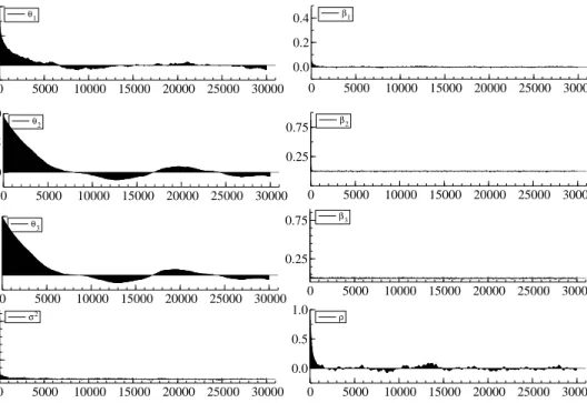
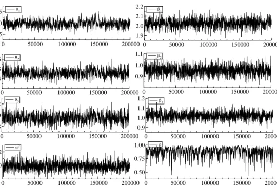
The initial 20,000 variates are discarded as so-called burn-in period and the subsequent 200,000 values are recorded to conduct an inference. Figure 1 & 2 show the sample paths and the sample autocorrelations functions for the benchmark Gibbs sampler A described in Section 2. It is clear that the sample paths show very slow convergence to the posterior distribution forθ′
is, parameters
of selection equation (1), and their autocorrelations do no decay even at 10,000 lags.
The summary statistics are given in Table 1. The inefficiency factors in Table 1 are calculated to measure how well the chain mixes. The inefficiency factor is defined as 1 + 2P∞s=1ρs where ρs
is the sample autocorrelation at lag s calculated from the sampled values (see e.g. Chib (2001)). It is the ratio of the numerical variance of the sample posterior mean to the variance of the sample mean from the hypothetical uncorrelated draws.
The inefficiency factors for θi’s are quite large in the range of 1600∼4900 for the benchmark
Gibbs sampler A and 900 ∼ 3300 for the benchmark Gibbs sampler B. The sampler B seems to be more efficient than the sampler A, but both samplers suffer from the poor mixing properties. This implies that we need to sample from the Gibbs sampler A about 4900 as many times as the hypothetical uncorrelated sampler to obtain the same variance of the posterior sample mean. We note that the corresponding factors forσ2 and ρ are also large, while those for β′
is, parameters of
0 50000 100000 150000 200000 0.5 1.0 1.5 θ 1 0 50000 100000 150000 200000 4 5 6 θ 2 0 50000 100000 150000 200000 8 10 12 θ3 0 50000 100000 150000 200000 1.9 2.0 2.1 2.2 β 1 0 50000 100000 150000 200000 0.9 1.0 1.1 β 2 0 50000 100000 150000 200000 1.0 1.1 β3 0 50000 100000 150000 200000 0.8 1.0 1.2 σ2 0 50000 100000 150000 200000 0.50 0.75 1.00 ρ
Figure 1: Sample paths from the benchmark Gibbs sampler A.
0 5000 10000 15000 20000 25000 30000 0.0 0.5 1.0 θ 1 0 5000 10000 15000 20000 25000 30000 0.0 0.5 1.0 θ2 0 5000 10000 15000 20000 25000 30000 0.0 0.5 1.0 θ 3 0 5000 10000 15000 20000 25000 30000 0.0 0.2 0.4 β1 0 5000 10000 15000 20000 25000 30000 0.25 0.75 β2 0 5000 10000 15000 20000 25000 30000 0.25 0.75 β3 0 5000 10000 15000 20000 25000 30000 0.25 0.75 σ2 0 5000 10000 15000 20000 25000 30000 0.0 0.5 1.0 ρ
True Mean Stdev 95% Interval Inefficiency A/B θ1 1.0 0.971 0.149 (0.687, 1.269) 1642.1/974.7 θ2 5.0 4.593 0.397 (3.875, 5.419) 4679.4/3090.8 θ3 10.0 9.508 0.800 (8.104, 11.167) 4840.5/3273.1 β1 2.0 2.027 0.043 (1.942, 2.112) 38.7/14.3 β2 1.0 0.951 0.042 (0.870, 1.034) 20.0/12.6 β3 1.0 1.019 0.039 (0.944, 1.095) 60.5/16.9 σ2 1.0 0.989 0.061 (0.877, 1.114) 193.3/120.1 ρ 0.9 0.882 0.080 (0.684, 0.985) 526.9/214.2
Table 1: Posterior means, standard deviations, 95% credible intervals are obtained from the benchmark Gibbs sampler A. Inefficiency factors are obtained from the benchmark Gibbs sampler A & B (ρ= 0.9).
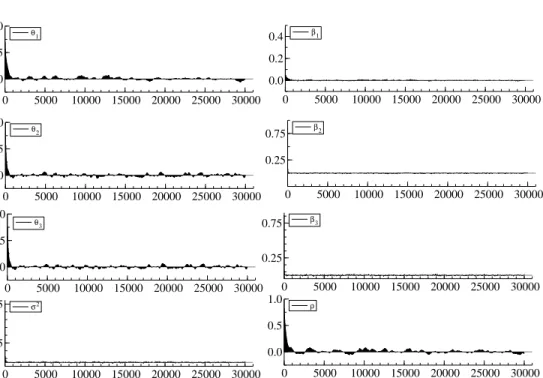
For the accelerated Gibbs sampler A described in Section 3.1, Figure 3 & 4 show the sample paths and sample autocorrelation functions. The sample paths seem to mix well and autocorre-lations die out very quickly. We skipped only 4.2 percent of the acceleration steps due to slow random generations, and succeeded in improving the mixing property of obtained samples. The summary statistics are shown in Table 2. The inefficiency factors for θ′
isare drastically decreased
to 250∼600 for the sampler A and 150∼230 for the sampler B.
0 50000 100000 150000 200000 0.5 1.0 1.5 θ1 0 50000 100000 150000 200000 4 5 6 θ2 0 50000 100000 150000 200000 8 10 12 θ3 0 50000 100000 150000 200000 1.9 2.0 2.1 2.2 β 1 0 50000 100000 150000 200000 0.9 1.0 1.1 β2 0 50000 100000 150000 200000 0.9 1.0 1.1 1.2 β3 0 50000 100000 150000 200000 1.0 1.2 σ 2 0 50000 100000 150000 200000 0.50 0.75 1.00 ρ
0 5000 10000 15000 20000 25000 30000 0.0 0.5 1.0 θ 1 0 5000 10000 15000 20000 25000 30000 0.0 0.5 1.0 θ2 0 5000 10000 15000 20000 25000 30000 0.0 0.5 1.0 θ3 0 5000 10000 15000 20000 25000 30000 0.0 0.2 0.4 β1 0 5000 10000 15000 20000 25000 30000 0.25 0.75 β2 0 5000 10000 15000 20000 25000 30000 0.25 0.75 β3 0 5000 10000 15000 20000 25000 30000 0.25 0.75 σ2 0 5000 10000 15000 20000 25000 30000 0.0 0.5 1.0 ρ
Figure 4: Sample autocorrelations from accelerated Gibbs sampler A.
True Mean Stdev 95% Interval Inefficiency
A/ B θ1 1.0 0.969 0.152 (0.681, 1.278) 557.6/215.8 θ2 5.0 4.589 0.399 (3.831, 5.389) 252.2/155.3 θ3 10.0 9.503 0.812 (7.967, 11.151) 252.7/150.1 β1 2.0 2.027 0.043 (1.941, 2.112) 47.4/12.7 β2 1.0 0.952 0.041 (0.871, 1.034) 34.4/12.1 β3 1.0 1.019 0.039 (0.943, 1.096) 17.9/12.5 σ2 1.0 0.988 0.061 (0.876, 1.113) 32.6/24.4 ρ 0.9 0.881 0.080 (0.686, 0.982) 598.8/230.0
Table 2: Posterior means, standard deviations, 95% credible intervals are obtained from the accelerated Gibbs sampler A. Inefficiency factors are obtained from the accelerated Gibbs sampler A & B (ρ= 0.9).
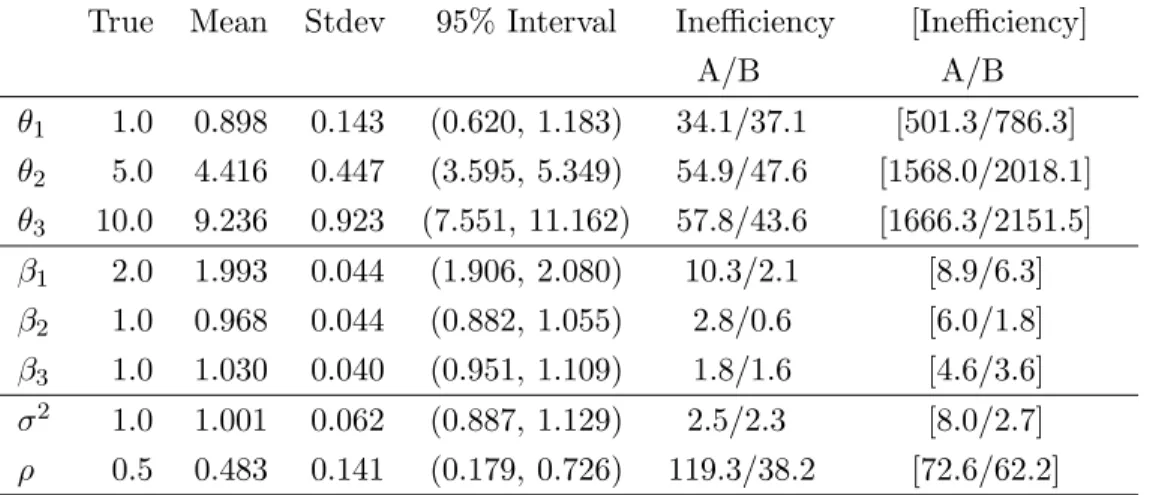
To investigate the influence of the correlation coefficient,ρ,on the sampling efficiencies, we repeated the experiments usingρ= 0.5 and 0.98.First, forρ= 0.5,Table 3 shows summary statistics for the accelerated Gibbs sampler A. The inefficiency factors of both samplers are still large for θ′
is, but
relatively smaller compared with those values in Table 1 & 2 with ρ = 0.9. The obtained samples seem to be less autocorrelated when the correlation coefficient ρ = 0.5. We did not need to skip any acceleration step due to slow random generations, and accomplished great improvements in decreasing the inefficiency factors.
For ρ= 0.98,Table 4 shows very high inefficiency factors forθ′
highly autocorrelated. Sinceρ is very close to one, we have very small values ofφ. This resulted in skipping 68.3% for the sampler A (50.4% for the sampler B) of acceleration steps due to the slow random number generations from theGIG(ν1/2, a, b) distribution, and we were not as successful as
in the case ρ= 0.5 or ρ= 0.9.
True Mean Stdev 95% Interval Inefficiency [Inefficiency] A/B A/B θ1 1.0 0.898 0.143 (0.620, 1.183) 34.1/37.1 [501.3/786.3] θ2 5.0 4.416 0.447 (3.595, 5.349) 54.9/47.6 [1568.0/2018.1] θ3 10.0 9.236 0.923 (7.551, 11.162) 57.8/43.6 [1666.3/2151.5] β1 2.0 1.993 0.044 (1.906, 2.080) 10.3/2.1 [8.9/6.3] β2 1.0 0.968 0.044 (0.882, 1.055) 2.8/0.6 [6.0/1.8] β3 1.0 1.030 0.040 (0.951, 1.109) 1.8/1.6 [4.6/3.6] σ2 1.0 1.001 0.062 (0.887, 1.129) 2.5/2.3 [8.0/2.7] ρ 0.5 0.483 0.141 (0.179, 0.726) 119.3/38.2 [72.6/62.2]
Table 3: Accelerated Gibbs sampler A when ρ = 0.5. Inefficiency factors using the benchmark Gibbs sampler A are given in brackets.
True Mean Stdev 95% Interval Inefficiency [Inefficiency] A/B A/B θ1 1.0 0.991 0.106 (0.765, 1.192) 692.5/830.2 [2295.2/3632.2] θ2 5.0 4.643 0.316 (3.960, 5.285) 1000.1/1486.4 [7601.9/8202.1] θ3 10.0 9.419 0.642 (8.053, 10.800) 1144.7/1474.6 [8256.1/8310.3] β1 2.0 2.038 0.042 (1.955, 2.122) 41.24/27.6 [46.4/27.3] β2 1.0 0.957 0.040 (0.879, 1.036) 158.8/124.6 [335.4/185.9] β3 1.0 1.003 0.037 (0.931, 1.076) 120.0/211.8 [603.9/264.6] σ2 1.0 0.995 0.059 (0.886, 1.117) 297.2/238.4 [683.4/1497.1] ρ 0.98 0.976 0.031 (0.887, 0.999) 909.8/845.4 [1142.0/967.0]
Table 4: Accelerated Gibbs sampler A (ρ= 0.98). Inefficiency factors using the benchmark Gibbs sampler A are given in brackets.
Since the inefficiency factors forθ1 are found to be smaller than those forθ2 andθ3, the above
experiments are repeated using different set of parameters forθ.We found that the inefficiency of the benchmark Gibbs sampler may become moderate when the values of θi are sufficiently small.
5
Conclusion
The efficient Markov chain Monte Carlo implementations are described for Bayesian analysis of a sample selection model. The proposed estimation method is illustrated using numerical examples
and is found to be highly efficient.
Acknowledgement. This work is supported by the Grants-in-Aid for Scientific Research 18330039
from the Japanese Ministry of Education, Science, Sports, Culture and Technology. The author thanks Nobuhiro Yoneda, Hideo Kozumi and the anonymous referees for their helpful comments and discussions.
Appendix A
A1 Gibbs sampler A
In this section we derive some formulas. Recall the definition (3). Conditional posterior probability density of φ.
π(φ|y∗c,z∗,θ,β, γ,yo) ∝ φ− n1 2 +1 exph− 1 2φ n γ2 n X i=1 (zi∗−wi′θ)2−2γ n X i=1 (zi∗−w′iθ)(yi∗−x′iβ) + n X i=1 (y∗i −x′iβ)2+S0 oi ∝ φ− n1 2 +1 expn− S1 2φ o .
Conditional posterior probability density of γ. π(γ|y∗c,z∗,θ,β, φ,yo) ∝ exph− 1 2φ n γ2 n X i=1 (zi∗−w′iθ)2−2γ n X i=1 (z∗i −wi′θ)(y∗i −x′iβ)o−(γ−γ0) 2 2G0 i ∝ expn−(γ−γ1) 2 2G1 o .
Conditional posterior probability density of ψ= (θ′,β′)′.
π(ψ|y∗c,z∗, γ, φ,yo) ∝ expn− 1 2 n X i=1 ( ˜y∗i −X˜iψ)′Σ−1( ˜y∗i −X˜iψ)− 1 2(ψ−ψ0) ′Ψ−1 0 (ψ−ψ0) o ∝ expn− 1 2(ψ−ψ1) ′Ψ−1 1 (ψ−ψ1) o .
A2 Gibbs sampler B
Conditional posterior probability density of φ:
π(φ|z∗,θ,β, γ,yo) ∝ φ− m1 2 +1 exph− 1 2φ n γ2 X i:z∗ i≥0 (z∗ i −w′iθ)2−2γ X i:z∗ i≥0 (z∗ i −w′iθ)(yi−x′iβ) + X i:z∗ i≥0 (yi−x′iβ)2+S0 oi ∝ φ− m1 2 +1 expn−S † 1 2φ o . where S1†=S0+γ2 n X i:z∗ i≥0 (zi∗−w′iθ)2−2γ X i:z∗ i≥0 (zi∗−w′iθ)(yi−x′iβ) + X i:z∗ i≥0 (yi−x′iβ)2.
Conditional posterior probability density of γ :
π(γ|z∗,θ,β, φ,yo) ∝ exph− 1 2φ n γ2 X i:z∗ i≥0 (zi∗−wi′θ)2−2γ X i:z∗ i≥0 (zi∗−wi′θ)(yi−x′iβ) o −(γ−γ0) 2 2G0 i ∝ expn−(γ−γ † 1)2 2G†1 o whereγ1†=G†1nG0−1γ0+φ−1Pi:z∗ i≥0(z ∗ i −wi′θ)(yi−x′iβ) o ,G†−1 1=G−01+φ−1P i:z∗ i≥0(z ∗ i −wi′θ)2.
Conditional posterior probability density of ψ= (θ′,β′)′.
π(ψ|z∗, γ, φ,yo) ∝ expn−1 2 X i:z∗ i≥0 ( ˜y†i −X˜i†ψ)′Σ−1( ˜yi†−X˜i†ψ)−1 2 X i:z∗ i<0 ( ˜y†i −X˜i†ψ)′( ˜yi†−X˜i†ψ) −1 2(ψ−ψ0) ′Ψ−1 0 (ψ−ψ0) ) ∝ expn−1 2(ψ−ψ1) ′Ψ−1 1 (ψ−ψ1) o ,
whereψ0, Ψ are as in (3) and
Ψ†1 = Ψ−01+ X i:z∗ i≥0 ˜ Xi†′Σ−1X˜i†+ X i:z∗ i<0 ˜ Xi†′X˜i†−1,
ψ†1 = Ψ†1Ψ−01ψ0+ X i:z∗ i≥0 ˜ Xi†′Σ−1y˜i†+ X i:z∗ i<0 ˜ Xi†′y˜†i ˜ y†i = ( (z∗ i, yi)′ ifzi∗≥0, (z∗ i,0)′ ifzi∗<0, ˜ Xi† = wi′ 0′ 0′ x′ i ! , ifz∗ i ≥0, wi′ 0′ 0′ 0′ ! , ifz∗ i <0.
Appendix B
Proof of Theorem 3.1. Given the current sample g of the conditional distribution, let α(g, g′)
denote the acceptance probability of the candidate g′ whereg′2 ∼ GIG(ν
1/2, a, b),
α(g, g′) = minhexpn(g′−g)(θ′Θ−1
0 θ0+γγ0G−01)
o
,1i.
Then the Markov transition function of g is Tx(g, g′)L(dg′) given parameters x = (√φ, γ,θ,z∗)
where Tx(g, g′) = (b/a) ν1 2 Kν1/2(ab) g′ν1 expn−1 2 a2g′−2+b2g′2oα(g, g′). Since Tg−1 0 (x)(gg0, g ′g 0) = { (b/g0)/(ag0)} ν1 2 Kν1/2((ag0)(b/g0)) (g′g 0)ν1 ×expn−1 2 (ag0)2g′−2g0−2+ (b/g0)2g′2g20 o αg−1 0 (x)(gg0, g ′g 0) = Tx(g, g′),
the result follows by Theorem 2 in Liu and Sabatti (2000).
References
Albert, J. and Chib, S. (1993), “Bayesian analysis of binary and polychotomous response data,” Journal of the American Statistical Association, 88, 669-679.
Amemiya, T. (1984), “Tobit models, a survey,” Journal of Econometrics,24, 3-61.
Barndorff-Nielsen, O. E. and Shephard, N. (2001), “Non-Gaussian Ornstein–Uhlenbeck-based models and some of their uses in financial economics (with discussion) ,” Journal of the Royal Statistical Society, Series B,63, 167-241.
Economet-rics, 51, 79-99.
Chib, S. (2001), Markov chain Monte Carlo methods: computation and inference. in J.J. Heckman and E. Leamer (eds.),Handbook of Econometrics,5, 3569-3649. North Holland, Amsterdam.
Chib, S. and Greenberg, E. (1995), “Understanding the Metropolis-Hastings algorithm,”American Statistician, 49, 327-335.
Chib, S. (2007), “Analysis of treatment response data without the joint distribution of potential outcomes,”Journal of Econometrics, in press.
Chib, S., Greenberg, E. and I Jeliazkov (2006), “Estimation of semiparametric models in the presence of endogeneity and sample selection,” Discussion paper, Olin School of Business, Washington University, St. Louis.
Dagpunar, J. S. (1989), “An easily implemented generalized inverse Gaussian generator,” Com-munications in Statistics-Simulations, 18, 703-710.
Doornik, J.A. (2002), Object-Oriented Matrix Programming Using Ox, 3rd ed. London: Timber-lake Consultants Press and Oxford: www.nuff.ox.ac.uk/Users/Doornik.
H¨ormann, W., Leydold, J. and Derflinger G. (2004), Automatic Nonuniform Random Variate Generation. Springer, Berlin.
Liu, J. S. and Sabatti, C. (2000), “Generalised Gibbs sampler and multigrid Monte Carlo for Bayesian computation,” Biometrika,87, 353-369.
Tierney, L. (1994), “Markov chains for exploring posterior distributions (with discussion),”Annals of Statistics,22, 1701-1762.
Tobin, J. (1958), “Estimation of relationships for limited dependent variables,Econometrica, 26, 24-36.