Kernel-Based Data Mining Approach with Variable Selection for Nonlinear High-Dimensional Data

(1)

University of Tennessee, Knoxville

Trace: Tennessee Research and Creative

Exchange

Doctoral Dissertations Graduate School

5-2010

Kernel-Based Data Mining Approach with Variable

Selection for Nonlinear High-Dimensional Data

Seung Hyun Baek

University of Tennessee - Knoxville, [email protected]

This Dissertation is brought to you for free and open access by the Graduate School at Trace: Tennessee Research and Creative Exchange. It has been

Recommended Citation

Baek, Seung Hyun, "Kernel-Based Data Mining Approach with Variable Selection for Nonlinear High-Dimensional Data. " PhD diss., University of Tennessee, 2010.

(2)

To the Graduate Council:

I am submitting herewith a dissertation written by Seung Hyun Baek entitled "Kernel-Based Data Mining Approach with Variable Selection for Nonlinear High-Dimensional Data." I have examined the final electronic copy of this dissertation for form and content and recommend that it be accepted in partial fulfillment of the requirements for the degree of Doctor of Philosophy, with a major in Industrial Engineering.

Alberto Garcia, Yuanshun Dai, Major Professor We have read this dissertation and recommend its acceptance:

Xiaoyan Zhu, Hamparsum Bozdogan, Adam M. Taylor

Accepted for the Council: Dixie L. Thompson Vice Provost and Dean of the Graduate School (Original signatures are on file with official student records.)

(3)

To the Graduate Council:

I am submitting herewith a dissertation written by Seung Hyun Baek entitled “Kernel-Based Data Mining Approach with Variable Selection for Nonlinear High-Dimensional Data.” I have examined the final electronic copy of this dissertation for form and content and recommend that it be accepted in partial fulfillment of the requirements for the degree of Doctor of Philosophy, with a major in Industrial Engineering.

Alberto Garcia Co-Advisor Yuanshun Dai Co-Advisor

We have read this dissertation and recommend its acceptance:

Xiaoyan Zhu

Hamparsum Bozdogan

Adam M. Taylor

Accepted for the Council:

Carolyn R. Hodges Vice Provost and

Dean of the Graduate School (Original signatures are on file with official student records.)

(4)

A Dissertation

Presented for the

Doctor of Philosophy Degree

The University of Tennessee, Knoxville

Seung Hyun Baek

May 2010

Kernel-Based Data Mining Approach with

Variable Selection for Nonlinear

(5)

(6)

Dedication

This dissertation is dedicated to my late father Tae Ho Baek (1945-2009), who passed away in a young age without seeing my success in finishing my degree. I also wish to dedicate this dissertation to my mother, Hee Suk Lim, who continually encouraged me to pursue my education and sacrificed many things for me so that one day I would become an honorable and educated citizen of this world. I have learned much about life from them. They have been my role-models for hard work, persistence and instilled in me the inspiration to set high goals and the confidence to achieve my future goals. I am dedicated to deliver their expectations in my life throughout my future.

(7)

ACKNOWLEDGEMENTS

I owe thanks to many people, whose assistance was indispensable in completing this dissertation. I wish to thank Dr. Alberto Garcia, and Dr. Yuanshun Dai, who served as my co-advisors and Ph.D. committee co-chairs, who helped me during the writing of my dissertation and provided support throughout in finishing my dissertation. I thank my mentor, Dr. Hamparsum Bozdogan for his cooperation and passion in providing knowledge and improving my research in the area of statistical modeling, especially model selection with his own development of information measure of complexity criterion. I thank Dr. Adam Taylor for his consistent help in providing NIR data sets. I thank to my sisters, Ji Yeon Baek, Su Yeon Baek, and Mi Yeon Baek for giving me warm-hearted support during the years of my graduate studies. I thank to my peers and friends in supporting me to complete my doctoral degree. Without such support and feedback process or loop, it would have been impossible to maintain and fulfill my long journey to get my doctoral degree.

(8)

ABSTRACT

In statistical data mining research, datasets often have nonlinearity and high-dimensionality. It has become difficult to analyze such datasets in a comprehensive manner using traditional statistical methodologies. Kernel-based data mining is one of the most effective statistical methodologies to investigate a variety of problems in areas including pattern recognition, machine learning, bioinformatics, chemometrics, and statistics. In particular, statistically-sophisticated procedures that emphasize the reliability of results and computational efficiency are required for the analysis of high-dimensional data.

In this dissertation, first, a novel wrapper method called SVM-ICOMPPERF-RFE based on hybridized support vector machine (SVM) and recursive feature elimination (RFE) with information-theoretic measure of complexity (ICOMP) is introduced and developed to classify high-dimensional data sets and to carry out subset selection of the variables in the original data space for finding the best for discriminating between groups. Recursive feature elimination (RFE) ranks variables based on the information-theoretic measure of complexity (ICOMP) criterion.

Second, a dual variables functional support vector machine approach is proposed. The proposed approach uses both the first and second derivatives of the degradation profiles. The modified floating search algorithm for the repeated variable selection, with newly-added degradation path points, is presented to find a few good variables while reducing the computation time for on-line implementation.

(9)

Third, a two-stage scheme for the classification of near infrared (NIR) spectral data is proposed. In the first stage, the proposed multi-scale vertical energy thresholding (MSVET) procedure is used to reduce the dimension of the high-dimensional spectral data. In the second stage, a few important wavelet coefficients are selected using the proposed SVM gradient-recursive feature elimination (RFE).

Fourth, a novel methodology based on a human decision making process for discriminant analysis called PDCM is proposed. The proposed methodology consists of three basic steps emulating the thinking process: perception, decision, and cognition. In these steps two concepts known as support vector machines for classification and information complexity are integrated to evaluate learning models.

(10)

List of Tables

Table Page

Table 1: Kernel Functions... 15

Table 2: Top Subset Variables Selected with 20% Set Using SVM-RFE Ranking ... 31

Table 4: Subset Selection Based on ICOMPPERF with 20% Set (Polynomial: degree=3) 32 Table 5: Subset Selection Based on ICOMPPERF with 80% Set (Cauchy) ... 33

Table 8: Subset Selection Based on ICOMPPERF with 20% Set (Cauchy) ... 36

Table 9: Subset Selection Based on ICOMPPERF with 80% Set (Inv. Multi Quadratic)... 37

Table 10: Comparison Using Ionosphere Data with 20%/80% ... 39

Table 11: Comparison Using Ionosphere Data with 80%/20% ... 40

Table 12: Comparison Using Aorta Data with 20%/80%... 40

Table 13: Comparison Using Aorta Data with 80%/20%... 40

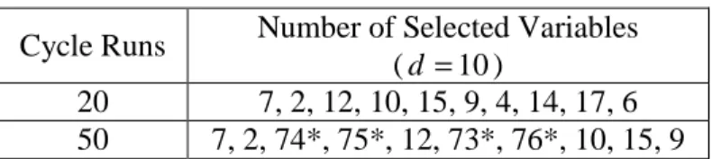
Table 14: Changes in Selected Variables Sets (* Second Derivative)... 55

Table 15: Classification Accuracy for Example 1 ... 74

Table 16: Classification Accuracy for Example 2 ... 76

Table 17: Classification Accuracy for Two Public Data Sets... 79

Table 18: Used Kernel Functions ... 91

Table 19: PDCM versus Various Ranking Based Method Using Cauchy... 95

Table 20: PDCM versus Various Ranking Based Method Using Inverse Multi-Quadratic ... 96

Table 22: PDCM versus Various Ranking Based Method Using Gaussian ... 98

Table 24: PDCM versus Various Ranking Based Method Using Inverse Multi-Quadratic ... 100

Table 25: Results for Antenna Curves (N = 128) ... 119

Table 26: Results for Tonnage Signals (N = 256) ... 120

Table 27: Results for Mallat Piecewise Signals (N = 1024) ... 122

Table 28: SNR Results for Antenna Curves ... 125

Table 29: SNR Results for Tonnage Signals ... 125

Table 30: SNR Results for Mallat Piecewise Signals (N=1024) ... 125

(15)

List of Figures

Figure Page

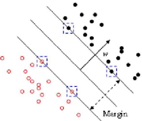
Figure 1: Illustration of Linear SVM for Nonlinearly Separable Case... 14

Figure 2: Grouped Scatter Plots for Ionosphere Data ... 30

Figure 3: Grouped Scatter Plots for Aorta Data... 34

Figure 4: Best Results of SVM-ICOMPPERF-RFE Using Ionosphere Data ... 41

Figure 5: Best Results of SVM-ICOMPPERF-RFE Using Aorta Data... 41

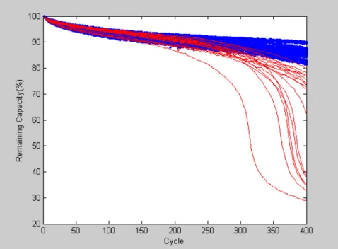
Figure 6: Remaining Capacities of Selected Battery Samples during Cycle-Life Tests .. 44

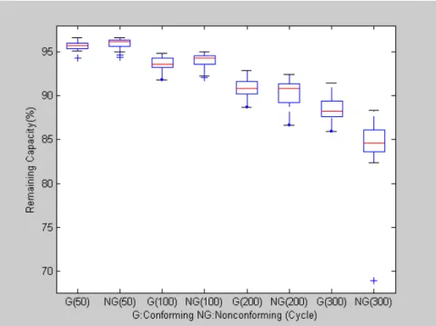
Figure 7: Box-Plots of Remaining Capacity at Some Cycles ... 46

Figure 8: Flowchart of the Dual Variables FSVM... 47

Figure 9: (a) First Derivatives of the Cycle-Life Curves (b) Second Derivatives of the Cycle-Life Curves (c) Classification with a First-First Derivative Combination (d) Classification with a First-Second Derivative Combination ... 49

Figure 10: Block Diagram of the Modified SFFS ... 51

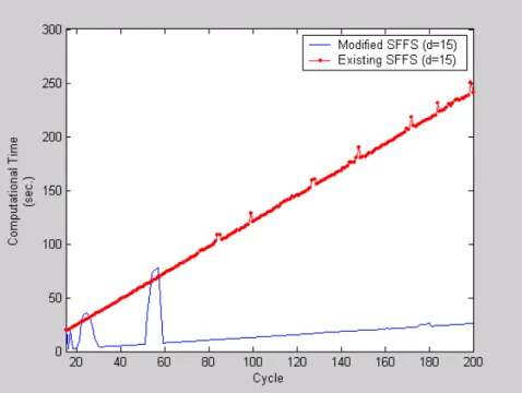
Figure 11: Computational Time for Selecting the Best Variables (d =15)... 56

Figure 12: Error Rate versus Cycle... 56

Figure 13: An Illustration of SVM for Two-Class Separation ... 61

Figure 14: A Schematic of the Proposed Two-Stage Framework ... 64

Figure 15: A Schematic Diagram of the Proposed MSVET Method ... 65

Figure 16: Original versus Reconstructed Data for Example 1 ... 73

Figure 17: A Plot for Classification Accuracy for Example 1... 74

Figure 18: A Plot for Classification Accuracy for Example 2... 75

Figure 19: Original versus Reconstructed Data for Example 2 ... 76

Figure 20: Classification Accuracy Plots for (a) Example 3 (b) Example 4 ... 78

Figure 21: Original versus Reconstructed Data for (a) Example 3 (b) Example 4... 79

Figure 22: Original and Reconstructed Data Curves ... 84

Figure 23: Classification Example Based on PDCM with SVM ... 91

Figure 24: Conceptual View of the Perception-Decision-Cognition Methodology ... 92

Figure 25: Antenna Data Curves... 119

Figure 26: Tonnage Signals ... 120

Figure 27: Mallat's Piecewise Signals ... 121

Figure 28: Antenna Data Curves... 123

Figure 29: Tonnage Signals. ... 124

(16)

Chapter 1 Introduction

This chapter provides an introduction of this dissertation research. Section 1.1 presents the motivation for the research. The contributions of the research are presented in Section 1.2. The organization of the rest of this dissertation is outlined in Section 1.3.

1.1 Motivation

Machine learning plays an important role in a variety of scientific fields including text mining, machine vision, pattern recognition, medical diagnosis, bioinformatics, and chemometrics. Practical problems arising in these fields require an approach built on innovative analytical methods. Two particularly important problems are (i) the presence of nonlinearities in available data; and (ii) the high-dimensionality of available data. In order to overcome these problems, kernel-based methods have been developed by several machine learning researchers. These methods are an effective alternative to increase computational power by first nonlinearly mapping the data into a high-dimensional space to avoid nonlinearities and then applying learning machines (modeling procedures). The objective of this dissertation is to develop innovative and effective analytical methods to increase computational power and improve scalability of complex data structures by (i) nonlinearly mapping the data into a high-dimensional space avoiding nonlinearities; and (ii) selecting the most relevant and informative variables.

Kernel-based methods exploit both the geometric and regularizing properties of a high-dimensional reproducing kernel Hilbert space. Since the early 1990s, kernel-based

(17)

methods have been built in several developments, including (a) support vector machine for both classification and regression (Boser et al. 1992; Vapnik 1995); (b) kernel principal component analysis (Schölkopf et al. 1999); and (c) kernel fisher discriminant analysis (Mika et al. 1999). Perhaps the best-known kernel-based method is the support vector machine, which has been successfully applied in a diverse range of domains. Several recent publications describe the application of kernel-based methods and address their overall performance in terms of computational requirements and ability, for both classification and regression (Cristianini and Shawe-Taylor 2000, Herbrich 2002, Schölkopf and Smola 2002, Vapnik 1995). The properties of a support vector machine are (i) managing large input spaces powerfully with kernel-based methods; (ii) dealing with noisy samples in a robust way; and (iii) producing sparse solutions (Chistianini and Shawe-Taylor 2000). Support vector machine can be incorporated with the scheme of the kernel-based methods. The kernel-based methods are based on mapping data from the original input space to a kernel space with high-dimensionality and then solving the problem in that space which is nonlinearly related to the input space. A kernel is a function K, such that for all ,x y∈X satisfies that K_Φ( , )x y =< Φ( ),x Φ( )y >, where Φ is a mapping from X to an inner product feature space F . The purpose of using the kernel function is as follows: (i) it provides the connection between the data and the modeling method; (ii) it can influence the performance of the modeling method by incorporating prior knowledge about the problem domain; and (iii) its evaluation might be computationally advantageous compared to an explicit construction of the feature space (Bloehdorn and Sure 2008).

(18)

Variable selection is an important area of research in machine learning, pattern recognition, statistics, and related fields. The key idea of variable selection is to find input variables which have predictive information and to eliminate non-informative variables. Variable selection identifies a small subset of variables so that the classifier constructed with the selected variables minimizes error and the selected variables also better explain the data (Koller and Sahami 1996). The use of variable selection techniques is motivated by three reasons: (i) to improve discrimination power; (ii) to find fast and cost-effective variables; and (iii) to reach a better understanding of the application process (Guyon and Elisseeff 2003). In the case of high-dimensionality data, variable selection plays a crucial role because of four challenges (Theodoridis and Koutroumbas 2006): (i) large sets of variables; (ii) existence of irrelevant variables; (iii) presence of redundant variables; and (iv) data noise.

1.2 Contributions of the Dissertation

Based on the motivations in Section 1.1, the contributions of this dissertation are as follows:

1. Hybridized support vector machine and recursive feature elimination with

information complexity: An innovative approach is proposed by taking advantages

from both the variable ranking method and the robust kernel-based method. This new approach is the hybridized support vector machine and recursive feature elimination with information complexity.

(19)

2. Dual variable functional support vector machine: Data representation for

functional structures is one of the key issues in implementing the functional support vector machine. In some cases, a combination of derivatives with different orders may lead to better classification performance. The dual variables functional support vector machine approach that uses both first and second derivatives.

3. Improved floating search method to optimize the number of variables: Because

dual or multiple data representations leads to a higher-dimension space, the modified floating search finds the optimal variables that have the highest classification power, so as to start with the best variable set in time series data.

4. Multi-scale vertical energy thresholding wavelet method based on the scale

information: The multi-scale based wavelet transformation can extract useful

information in compressed wavelet coefficients and thus can be used to perform noise suppression and pre-processing.

5. Two-stage scheme for incorporating a wavelet de-noising and reduction method

with a support vector machine-based variable selection method: The use of the

concentrated information with selected variables, instead of full variables, for the classification of high-dimensional data, can minimize classification error and improve computation speed significantly.

6. Perception-decision-cognition methodology for discriminant analysis based on

the human decision-making process: The proposed methodology consists of three

basic steps that emulate the thinking process: perception, decision, and cognition. In these steps two concepts known as the support vector machine and information complexity are integrated to evaluate learning models.

(20)

1.3 Outlines of the Dissertation

The remainder of this dissertation is organized as follows:

Chapter 2 shows a novel wrapper method based on hybridized support vector machine and recursive feature elimination with information complexity to classify nonlinear high-dimensional data sets and to carry out subset selection of the variables in the original data space.

In Chapter 3, a dual variable functional support vector machine and modified floating search based variable selection are presented. The different pre-processing techniques and the floating search method are explained.

Chapter 4 shows a two-stage classification procedure based on multi-scale vertical energy wavelet thresholding and support vector machine-based gradient recursive feature elimination. A wavelet-based data compression and de-noising technique and a support vector machine-based variable ranking algorithm are presented in detail.

In Chapter 5, a novel methodology based on the human decision-making process for discriminant analysis is presented. The proposed methodology consists of three basic steps emulating the thinking process: perception, decision, and cognition.

(21)

Chapter 2 Hybridized Support Vector

Machine and Recursive Feature

Elimination with Information Complexity

2.1 Introduction

In many classification problems there are very high-dimensional input data sets and finding the best subset of the original input features or variables which mostly contribute to the separation of the classes or groups is a challenge. Therefore, variable selection is a difficult combinatorial problem in machine learning and it has very high practical importance in many applications.

Kernel-based methods have gained popularity for classification, clustering, and regression analysis in machine learning since the introduction of support vector machine (SVM) during the early 1990s. After obtaining support vectors (SVs) to classify a data set, questions such as: “How do we know which variables are more responsible for, and important to, the classification?” have often been raised. This is due to the fact that the mapping is not one-to-one and onto in SVM. The application of a kernel function is thus an uninvertible process, and there is no way to go from the feature space back to the original space. Because of this geometry, SVM does not lend itself to automated internal relevant variable selection easily. Hence algorithms for variable selection play an important role in SVM.

(22)

In the literature of machine learning, as discussed in Fröhlich (2002) in detail, there are two main approaches to solve the variable selection problem: (a) the filter approach, and (b) the wrapper approach. Both approaches differ in the way they evaluate a given variable subset. The filter method uses some relevance measure, which is independent of the performance of the learning algorithm. On the other hand, in the wrapper method, each variable subset is taken into consideration with the classifier. That is, the variables are evaluated by estimating the generalization performance (i.e. the expected risk) of the learning machine trained.

In this chapter, the wrapper method called SVM-ICOMPPERF-RFE, which combines an information-theoretic measure of complexity (ICOMP) criterion and recursive feature elimination especially designed for SVM based variable selection developed by Guyon et al. (2002) is considered and emphasized. In the usual RFE, backward variable elimination is performed to find say, m, variables which lead to the largest margin of class separation. This combinatorial problem is solved in a greedy fashion. In the two-class case the RFE algorithm begins with the set of all variables and sequentially evaluates each variable based on sensitivity analysis for an appropriately defined criterion that is a measure of predictive ability (and is inversely proportional to the margin). Then, the RFE algorithm at each step eliminates the variable which keeps this quantity small. Assuming the change of the set of support vectors when removing only one variable is negligible.

An information-theoretic measure of complexity (ICOMP) criterion of Bozdogan (1988a, 1988b, 1990, 1994, 2000) is used in RFE rankings of the variables as an effective measure. ICOMP plays an important role not only in choosing an optimal kernel function

(23)

from a portfolio of many other kernel functions but also in selecting important subset(s) of variables. It takes into account either the badness of fit or the lack of fit and the model complexity at the same time in one criterion function.

The potential and the flexibility of the proposed method is illustrated on two real data sets, one is ionosphere data which includes radar returns from the ionosphere, and another is aorta data which is used for the early detection of atheroma most commonly resulting heart attack. Also, the proposed method is compared with other RFE based methods (Guyon et al. 2002; Youn 2002; Cho et al. 2009) using different measures (i.e., weight and gradient) for variable rankings.

2.2 Support Vector Machine

The SVM finds the optimal separable hyperplane that maximizes the margin between the classes (Vapnik 1995). Consider the case of classifying a set of training data into two groups. Assume a set of training data is given by

{

(

x y

) (

⋯ x_n y_n

)

}

1, 1 , , , where i

x is an input vector, y_i∈ −( 1,1) is a binary class index, and n is the size of training data. Then, a decision boundary (i.e. classifier) that partitions the underlying vector space into two classes can be represented by the following hyperplane:

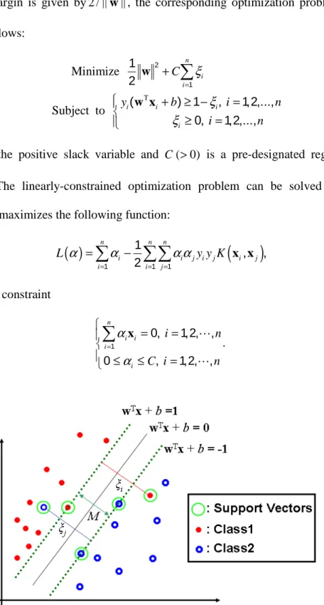
w xT + =b 0, (1) where w is the weight vector and b is the bias. The objective of the SVM is to find the maximum margin(M) decision boundary between the two parallel hyperplanes,

T b + = w x 1 and T b + = −

(24)

maximum margin is given by 2 / ||w , the corresponding optimization problem can be || written as follows: _T Minimize Subject to n i i i i i i C y b i n i n ξ ξ ξ = +  _{+ ≥ −} ₌   ≥ = 

∑

w w x 2 1 1 2 ( ) 1 , 1,2,..., 0, 1,2,..., (2)

where ξi is the positive slack variable and C(>0) is a pre-designated regularization coefficient. The linearly-constrained optimization problem can be solved as a dual problem that maximizes the following function:

( )

(

)

n n n i i j i j i j i i j L α α α α y y K = = = =

∑

−

∑∑

x x 1 1 1 1 , , 2 (3)

subject to the constraint

. n i i i i i n C i n α α =  = =    _≤ _≤ ₌ 

∑

x ⋯ ⋯ 1 0, 1,2, , 0 , 1,2, , (4)

(25)

Once the optimum values

(

α*,b*

)

are obtained, based upon the training set of points, a new point x_new of the test data set is classified by the following decision rule:

( )

Class 1 if Class 2 if n new i i i new i n new i i i new i D y K b D y K b α α = =  = + <     ₌ ₊ _> 

∑

x x x x x x * * 1 * * 1 ( , ) 0 ( , ) 0 (5)

where D

( )

i _{is a classifier based upon the training data set.}

i new

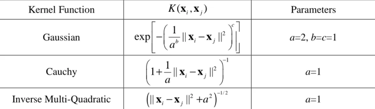
K x x( , ) is the kernel trick proposed by Aizerman et al. (1964). The kernel maps input data in the original space with nonlinearly into a high-dimensional feature space with linearity. The Table 1 presents some common kernel functions.

2.3 Information-Theoretic Measure of Complexity

An information-theoretic measure of complexity called ICOMP has been proposed by

Bozdogan (1988a, 1988b, 1990, 2000) as a decision rule for model selection Table 1: Kernel Functions

Function K(X,Y) Parameters

Linear ( T )a b + X Y a=1, b=0 Polynomial (degree=2) ₍_{X Y}T +_b₎a a=2, b=1 Polynomial (degree=3) ( T )a b + X Y a=3, b=1 Gaussian _b c a − 1 X−Y 2 exp( ( || || ) ) a=2, b=c=1 Cauchy a − +1 X−Y 2 1 (1 || || ) a=1 Inverse Multi-Quadratic (||X−Y||2 +a2)−1/ 2 a=1

(26)

such as AIC (Akaike, 1973), and BIC (Schwarz, 1978). The development and construction of ICOMP is based on a generalization of the covariance complexity index originally introduced by van Emden (1971). Instead of penalizing the number of free parameters directly, ICOMP penalizes the covariance complexity of the model. It is defined by

ICOMP= −2 log (Lθˆk)+2 (C ΣˆModel), (6) where L(θˆ_k) is the maximized likelihood function, ˆθ_k is the maximum likelihood estimate of the parameter vector θ_k under the model M_k, and C represents a real-valued complexity measure and Cov(θˆ_k)=Σˆ_Model represents the estimated covariance matrix of the parameter vector of the model. ICOMP should not be confused with the stochastic complexity (SC) or the minimum description length (MDL) of Rissanen (1986, 1987, 1989), although they both use the notion of complexity of a model class based on coding theory. The detailed information-theoretic measure of complexity (ICOMP) is recapitulated in the subsections for the benefit of the readers who may not be familiar with ICOMP criterion.

2.3.1 Mutual Information in High Dimensions

For a random vector, the complexity is defined as follows.

Definition: The complexity of a random vector is a measure of the interdependency among its components.

A continuous p-variate distribution is used with joint density function

1

( ) ( ,..., p)

(27)

Kullback (1997), and Harris (1978), the information measure of dependence is defined as follows: 1 1 1 1 1 1 1 1 1 ( ,..., ) ( ) ( ,..., ) [log ] ( ) ( ) ( ,..., ) ( ,..., ) log ( ) ( ) p p f p p p p p p p f x x I I x x E f x f x f x x f x x dx dx f x f x +∞ +∞ −∞ −∞ = = =

_∫

x ⋯ ⋯ ⋯ ⋯ (7)

where

I x

( )

is the Kullback-Leibler information divergence (Kullback and Leibler 1951) against independence. The properties of the Kullback-Leibler information divergence are as follows:

• I( )x ≡I x( ,...,1 xp)≥0 i.e., the expected mutual information is nonnegative. • I( )x ≡I x( ,...,1 xp)=0 if and only if f x( ,...,1 xp)= f x1( )1 ⋯f xp( p) for every

p-tuple ( ,...,x₁ xp), i.e., if and only if the random variables x1,...,xpare mutually statistically independent.

The KL divergence is related to Shannon's entropy (Shannon 1948) by the important identity ₁ ₁ 1 ( ) ( ,..., ) ( ) ( ,..., ) p p j p j I I x x H x H x x = ≡ =

∑

− x (8) where

• H x( )j is the marginal entropy, and • H x( ,...,1 xp) is the global or joint entropy

Watanabe (1985) calls this latter quantity the strength of structure and a measure of inter-dependence.

(28)

To define the information-theoretic measure of complexity of a multivariate distribution, let f( )x = f x( ,...,1 xp) be a multivariate Gaussian density function given by

1 1 T 1 2 2 ( ) ( ,..., ) 1 (2 ) | | exp{ ( ) ( )}, 2 p p f f x x

π

− − − = = − − − x Σ x µ Σ x µ (9)

where µ=( ,

µ µ

₁ ₂,...,

µ

_p) ,T −∞ <

µ

_j < ∞ =,j 1, 2,...,pand Σ>0(positive definite) As a short hand, let

x~ N_p( , ).µ Σ (10) Then the joint entropy H( )x =H x( ,...,₁ x_p) from equation (8) for the case in which

µ

=

0

is given by 1 T 1 1 T ( ) ( ,..., ) ( ) log ( ) 1 ( ) log(2 ) | | ( ) ( ) 2 2 1 log(2 ) | | ( ) ( )( ) . 2 2 p p p p H H x x f f d p f d p tr f d

π

− −           = = − = + − − = + − −

∫

R R R x x x x x Σ x µ Σ x µ x Σ x Σ x µ x µ x (11)

Then, since E[(x−µ)(x−µ) ]T =Σ, the joint entropy is

1 1 ( ) ( ,..., ) log(2 ) log | | 2 2 2 1 [log(2 ) 1] log | | . 2 2 p p p H H x x p

π

= = + + = + + x Σ Σ (12)

From equation (11), the marginal entropy H x( )j is

2

( )

( ) log ( )

1

1 log(2 )

log(

),

1, 2,..., ,

2

j j j j j

H x

f x

f x dx

j

p

π

σ

+∞ −∞

= −

=

+ +

=

∫

(13)

(29)

2.3.2 Initial Definition of Covariance Complexity

van Emden (1971, p. 61) provides a reasonable initial definition of complexity of a covariance matrix Σ for the multivariate Gaussian distribution. This measure is given by: 1 0 1 1 1 ( ,..., ) ( ) ( ) ( ,..., ) 1 1 1 1

log(2 ) log( ) log(2 ) log | | .

2 2 2 2 2 2 p p j p j p jj j I x x C H x H x x p p

π

σ

π

= =       ≡ = − = + + − − −

∑

Σ Σ (14) This reduces to ₀ 1 1 1 ( ) log( ) log | |, 2 2 p jj j C

σ

= =

∑

− Σ Σ (15) where 2_, jj j

σ

≡

σ

is the variance of the jth variable, and is the jth diagonal element of

Σ

. The characteristics of covariance complexityC₀ are as follows:

• C₀( )

Σ

=0 if and only if Σ is a diagonal matrix. • C₀( )

Σ

= ∞ if and only if |Σ| 0= .

• The first term of equation (15) is not invariant under orthonormal transformations. As pointed out by van Emden (1971), the result in equation (15) is not an effective measure of the amount of complexity in the covariance matrix Σ, since:

• C₀( )Σ depends on the coordinates of the original random variables x₁,...,xp. • The first term of C₀( )Σ in equation (15) would change under orthonormal

(30)

2.3.3 Definition of Maximal Covariance Complexity

To improve upon C₀( )Σ in equation (15), a maximal covariance complexity is proposed as follows.

Proposition: A maximal information theoretic measure of complexity of a covariance matrix Σ of a multivariate Gaussian distribution is defined as follows:

1 0 1 1 log ( ) max ( ) max{ ( ) ( ) ( ,..., )} ( ) 1 log | | 2 2 λ log , 2 λ p p T T a g C C H x H x H x x p tr p p       = = + + − = − = Σ Σ Σ Σ ⋯ (16)

where the maximum is taken over the orthonormal similarity transformation, T of the overall coordinate systems x₁,...,xp and λaand λg are arithmetic and geometric means of the eigenvalues. The properties of maximal information-theoretic measure of complexity are as follows:

• C₁( )Σ is the log ratio between the arithmetic and geometric mean of the eigenvalues.

• C₁( )Σ incorporates the two most basic scalar measures of multivariate scatter-trace and determinant.

• C₁( )Σ →0 as Σ→Ip.

(31)

2.3.4 Modified Maximal Covariance Complexity

Following van Emden (1971), the geometric definition of covariance complexity is defined by the Frobenius norm given by

2 2 ,

1 ( )

( )

||

F

tr

C

s

     

=

−

Σ

(17) where 2 T

||Σ|| =tr(Σ Σ), the square of the Frobenius norm of Σ.

In terms of the eigenvalues (or singular values), CF( )Σ reduces to

2 1 1 ( ) (λ λ _{) ,} s j a F j C s = =

∑

− Σ (18)

where s is the rank of Σ, λ

jis the j th

eigenvalue of Σ> 0, j = 1,2,. . .,s and λ

ais arithmetic mean of the eigenvalues. Note that CF( )Σ ≥0 with CF( )Σ =0 only when all

λ λ _.

j = a 1( )

C Σ can be approximated in terms of the eigenvalues λ , 1, 2, , j j= … sby ₁ 2 1 . λ λ 1 ( ) ( ) 4 λ s j a j _a C = − ≅

∑

Σ (19)

Since in the feature space orthonormal matrices are dealt with to prevent the C₁

complexity not to go to zero, C₁ and C_F are related as a second order equivalent measure of complexity denoted byC1F . Hence, the modified maximal entropic complexity

1F( )

(32)

2 2 1 2 2 ( ) . ( ) ( )

1 ||

||

( )

4

F F tr s tr tr s s

C

s

s s

C

                 

−

=

Σ Σ Σ

Σ

(20)

In terms of the eigenvalues,

C

₁_F

( )

Σ

is given by

2 2 1 2 2 1 2 T 1 2 ( ) ( ) 1 (λ λ ₎ 4 λ 1 (λ λ _{) .} 4λ 1 ( ) ( ) 4 s j a j a s j a j a F tr s tr s s s tr s s C = =             = − = − − =

∑

Σ Σ Σ Σ Σ (21)

where

s

=

rank

( )

Σ

. The properties of the modified maximal entropic complexity C_1F

are as follows:

• C₁_F( )Σ is scale-invariant, and C₁_F( )Σ ≥0 with C₁_F( )Σ =0 only when all

λ

_.

j

=

a

• C₁_F

( )

Σ measures the relative variation in the eigenvalues rather than absolute variation of the eigenvalues.

2.3.5 ICOMP as a Performance Measure: ICOMPPERF

Singularity of the estimated covariance matrix is a common problem that has recently attracted many researchers’ work. Because of this, many methods have been proposed to make the covariance matrix well-conditioned, so that the covariance matrix can be estimated. The usual response to singular or ill-conditioned covariance matrix

(33)

estimates is the “naive” ridge regularization, Σˆ* =[Σˆ +

α

Ip], which works to counteract

the ill-conditioning by adjusting the eigenvalues of ˆΣ . The ridge parameter,α , is typically chosen to be very small. This, of course, begs the questions

• How large of a perturbation do we need?

• How small a perturbation can we get away with?

This is a case where simplicity is not necessarily a good thing; it does not solve the problem with many real datasets. Yet another approach that does not seem to work well in practice is to augment Σˆ with a multiple of the kernel matrix, as suggested by Mika (2002). After much experimentation with a variety of different methods to improve the condition of the covariance matrix, a stabilization method (Thomaz 2004) is applied to resolve the ill-conditioning of a covariance matrix. After the stabilization procedure, the two-stage stabilization and smoothing process is applied to provide a well-conditioned covariance matrix which is both nonsingular and positive definite.

• Stage 1. Stabilization algorithm (Thomaz 2004):

1. Perform spectral decomposition of

Σ

ˆ

=

V

Λ

V

T, where V is the matrix with eigenvectors and Λhas eigenvalues on the diagonal.

2. Calculate the mean eigenvalue p i=1

λ₌₍ λ

i p

∑

) /

3. Form a new matrix of eigenvalues as

= Λ* λ λ λ λ p           ⋯ ⋮ ⋱ ⋮ ⋯ 1 max( ) 0 0 max( ) , ,

(34)

T STA

=

Σ

ˆ

V

Λ

*

V

• Stage 2: Compute a Stabilized and Smoothed Convex Sum Covariance Estimator The second step is to feed the stabilized covariance matrix into a smoothed convex sum covariance matrix estimator (CSE) was proposed based on the quadratic loss function used by Press (1975) and later by Chen (1976). The stabilized and smoothed convex sum covariance estimator (STA-CSE) is as follows:

ˆ_{STA CSE}_{_} n ˆ_STA (1 n )ˆ_STA,

n m n m

= + −

+ +

Σ Σ D (22)

where

ˆ

STA

1 tr

(

ˆ

STA) p

p

     

=

D

Σ

I

. For p≥2, m is chosen to be 2[ (1 ) 2] 0 m p , p

β

+ − < < − where

(

)

2 2 ˆ ( ) . ˆ ( ) STA STA tr tr

β

= Σ Σ

This estimator improves upon Σˆ_STAby shrinking all the estimated eigenvalues of

ˆ

STA

Σ

toward their common mean. The motivation of using both stabilization and smoothing of the covariance matrix in the ranking process of RFE subset selection is to extract more information since a reduced rank problem occur in the kernel based methods. To remedy the current existing problems in the usual kernel methods, the use of both stabilization and smoothing the covariance matrix is an attractive approach.

The choice of the best mapping function is not so simple and automatic. In the literature a valid method for selecting the appropriate kernel function does not yet exist.

(35)

The goal of SVM is to minimize the probability of misclassification error. Intuitively, then, the penalty term for a poorly-fitting model would be based on the classification error rate. In SVM problems, the error variance

σ

2

is estimated by the mean squared difference between actual group labels (y_i) and predicted group labels (yˆ_i) given by

2 2 1 1 ˆ ( ˆ ) . n i i i y y n

σ

= =

∑

− (23) Now following the work of Howe and Bozdogan (2010) the information-theoretic measure of complexity as performance measure of SVM is defined as follows:

ICOMP_PERF =nlog 2π+nlog ˆσ2+ +n 2C₁_F(Σˆ_STA_{_}_CSE), (24) where

Σ

ˆ

_{STA CSE}_{_} is the stabilized and smoothed convex sum covariance matrix estimator (STA-CSE) given by

_ )

1 ˆ

ˆ

₍₁

₎

ˆ

_,

ˆ

₍

ˆ

_,

p

STA CSE STA STA STA STA

n

tr

n m

p

     

=

₊

+ −

₊

=

Σ

D

Σ

I

and 2 1 _ 2 1

1 ˆ

(

)

(

λ

_{) .}

4 λ

s j a F STA CSE j a

C

=

∑

−

Σ

First, the hybrid covariance estimate is calculated, and then the diagonal matrix of the largest singular values as a reduced rank approximation of

Σ

ˆ

_{STA CSE}_{_} is computed. By minimizing ICOMPPERF, the classification error is minimized under the best fitting model. Also, ICOMPPERF is used to choose an optimal kernel function. One of the major motivations of introducing the information measure of complexity (ICOMP) criterion is based on the fact that in SVM-RFE subset selection problems the number of variables is

(36)

same from one subset to another. In such cases the models in terms of the number of parameters are considered to be equivalent. In equivalent models, AIC, BIC, or MDL type criteria do not have provision of distinguishing one equivalent model from another. Since their penalty terms are fixed, and not varying. In the literature cross-validation-based criteria has been used for variable selection. These types of criteria are too time-consuming due to the high-dimensionality of the feature space. The proposed method shortens the variable selection time.

2.4 Recursive Feature Elimination (RFE)

A variable selection method based on RFE has been developed by Guyon et al. (2002) which is called SVM-RFE. SVM-RFE is an application of a recursive feature elimination based on sensitivity analysis using an appropriately defined cost function (w: weight). The SVM-Gradient-RFE method (Youn 2002; Cho et al. 2009) used the gradient as a cost function. In the proposed method, the used cost function is the ICOMPPERF. In the proposed method, the least sensitive variable, which has the minimum value of the ICOMPPERF, is eliminated first. This eliminated variable becomes rank p (p: number of variables). Later, the machine is retrained on the remaining p-1 variables and then the variable with the minimum value of ICOMPPERF is eliminated. The process continuous in an iterative fashion until no variable is left in that subset. This means that at the end of this iterative ranking scheme all the variables are ranked according to ICOMPPERF criterion. This is different than the Guyon et al. (2002) ranking scheme where only weights have been considered without taking into account the model fit and the complexity of the model.

(37)

2.4.1 SVM-RFE Algorithm

Let X=( ,...,x1 xn)T be a training set with

T n

y y

=

y ( ,...,1 ) .

1. Construct a training modelX= X(:, )s , where s is the subset of variables; s=1,2,…,p. 2. Until all values of the cost function are obtained with the number of non-ranked

variables, compute the cost function for all subsets

C i( )=(1/ 2)αTHα−(1/ 2)αTH(−i)α, (25) where H= y y K_i _j ( ,x x_i _j), and H(-i) means a H matrix without the ith variable. 3. Find the variable k with the smallest cost function value, and add k into the ranked

subset, r and remove k from subset, s.

4. Repeat 1-3 until subset, s is empty.

2.4.2 SVM-Gradient-RFE Algorithm

Let X=( ,...,x₁ x_n)Tbe a training set with y=( ,...,y1 yn) .T

1. Construct a training modelX= X(:, )s , s is the subset of variables; s=1,2,…,p.

2. Until all values of the average sum of the angles are obtained with the number of non-ranked variables,

(i) compute the gradient, ∇(-i)g(x) without ith variable sv i i m m m m g α y K − − ∈ ∇ x =

∑

∇ x x ( ) ( ) ( ) ( , ). (26) (ii) compute the sum of angles between ∇(-i)g(x) and e , m γ

sv i m m i g γ ₋ ∈ =

∑

∠ ∇ x e ( ) ( ) ( ( ), ), (27)

(38)

where (-i) means without the ith variable, e is unit vectors, and _m i i i m m g g g β β βπ − − − ∈   _∇   _ _ ∠ ∇ =  + − _ _ ∇  _ _   x e x e x i ( ) ( ) ( ) {0,1} ( ) ( ( ), ) min ( 1) arccos . || ( ) ||

(iii) compute the average sum of the angles

SV i A i γ π = −2i ( ) ( ) 1 . | |

3. Find the variable k with the smallest the average sum of the angle A(i), add k into the ranked subset, r and remove k from subset, s.

4. Repeat 1-3 until subset, s is empty.

2.4.3 Proposed SVM-ICOMPPERF-RFE Algorithm

Let X=( ,...,x1 x_n)Tbe a training set with

T n

y y

=

y ( ,...,1 ) .

1. Construct a training modelX= X(:, )s , where s is the subset of variables; s=1,2,…,p. 2. Until all ICOMPPERF values are obtained with the number of non-ranked variables,

compute ICOMPPERF based on the error rate obtained from SVM. The ICOMPPERF is given by

ICOMP_PERF( )i =nlog 2π+nlog ˆσ₍2₋_i₎+ +n 2C₁_F(Σˆ_{STA CSE}_{_} ₍₋_i₎), (28) where

σ

ˆ

₍2₋_i₎ is the estimated error variance without the ith variable and Σˆ_{STA CSE}_{_} ₍₋_i₎ is the stabilized and smoothed convex sum covariance matrix estimator without the ith variable in the model.

3. Find the variable k with the smallest ICOMPPERF, add k into the ranked subset, r and remove k from subset, s.

(39)

2.5 Numerical Results

In the data mining literature, data partitioning is an important issue for finding proper models for new datasets. In general one can use different data partitioning to get different results. Most of such data partitioning schemes do not take into account of randomness that may affect the performance of the results which can be different. In the analysis, to avoid partitioning dependency, the data is randomly partitioned into 20% as one set and 80% as another set based on Pareto’s principle (Pareto 1909). Two experiments are performed with two different sets; 20%/80% and vice versa as training/test sets. The variable rankings corresponding to kernel functions are determined and reported for those different sets. Also, the smallest value of ICOMPPERF, and the 95% confidence intervals (CIs) given byX_error ±1.96 ˆσ_error for the training and test errors are reported. Ionosphere and aorta datasets are used for these experiments.

2.5.1 Ionosphere Data

The ionosphere data are radar data which was collected by a system in Goose Bay, Labrador (Sigillito et al. 1989). The system measures radar returns from the ionosphere. The data consist of 351 observations and 34 variables with binary classes; good and bad returns. Figure 2 shows the scatter plots of the data with groups identified by blue (circle) and red (cross) colors. As shown in Figure 2, the separation in dimension 5 against dimensions 13, 19 and dimensions 18, 29 are quite poor. Tables 2 and 3 show performances of experiments based on ICOMPPERF. In Table 2, the polynomial kernel with degree 3 on the 20% set shows a narrower confidence interval than the other kernel

(40)

functions for both training and test sets. As shown in Tables 2 and 3, the smallest ICOMPPERF values are obtained with a polynomial kernel with degree 3 for the 20% set and the 80% set. Tables 4 and 5 show the best subset selection based on the smallest ICOMPPERF values. The training and test errors of the best subsets in both partitioned sets are within the 95% error confidence intervals.

-1 -0.5 0 0.5 1 -1 -0.5 0 0.5 1 -1 -0.8 -0.6 -0.4 -0.2 0 0.2 0.4 0.6 0.8 1 D im e n s io n 1 9 Dimension 5 Dimension 13 _-1 -0.5 0 0.5 1 -1 -0.5 0 0.5 1 -1 -0.8 -0.6 -0.4 -0.2 0 0.2 0.4 0.6 0.8 1 D im e n s io n 2 9 Dimension 5 Dimension 18

Figure 2: Grouped Scatter Plots for Ionosphere Data

(41)

Table 2: Top Subset Variables Selected with 20% Set Using SVM-RFE Ranking

Kernel Best Subset Best ICOMPPERF Training Error CI Testing Error CI

Linear {27,12} 121.14 [0.03046, 0.33089] [0.12241, 0.38356] Ranking {27,12,24,32,30,31,4,18,20,34,2,26,9,6,8,28,16,14,25,7,5,22,3,29,17,15,21,23,10,1,11,33,19,13} Cauchy {1-9,11-34} 87.61 [0.08101, 0.36773] [0.25495, 0.42540] Ranking {24,5,3,33,26,31,6,9,22,34,18,11,21,19,4,32,23,15,25,12,30,29,13,2,28,20,1,8,16,27,7,14,17,10} Polynomial (degree=2) {2-20,22-30,32-34} -47953.45 [0, 0.23670] [0.06150, 0.31593] Ranking {30,32,29,12,34,4,2,23,14,26,18,6,20,28,8,33,16,22,7,10,5,24,27,3,17,15,13,19,25,9,11,1,21,31} Polynomial (degree=3) {2,3,8,12-14,18,20,22,24-32} -47957.44 [0, 0.14278] [0.10669, 0.21464] Ranking {3,14,24,26,13,28,2,8,20,30,12,18,27,31,25,29,32,22,6,16,5,4,11,10,34,1,19,33,21,7,23,9,17,15}

Table 3: Top Subset Variables Selected with 80% Set Using SVM-RFE Ranking

Kernel Best Subset Best ICOMPPERF Training Error CI Testing Error CI

Linear {7} 606.94 [0.09676, 0.23190] [0.09271, 0.26610] Ranking {7,27,6,31,30,28,32,26,14,8,10,16,2,24,19,4,18,11,3,20,22,34,29,13,25,21,9,33,23,17,1,12,5,15} Cauchy {3} 441.65 [0.02329, 0.20342] [0, 0.38375] Ranking {3,6,4,7,8,5,1,18,14,10,16,12,13,2,24,9,19,15,17,23,21,31,29,25,22,33,34,28,32,30,26,20,11,27} Polynomial (degree=2) {5,14} 454.56 [0, 0.13966] [0, 0.18645] Ranking {5,14,8,16,10,22,32,29,31,3,27,12,34,4,7,20,23,26,25,19,15,9,17,13,33,24,21,28,11,30,6,18,2,1} Polynomial (degree=3) {5} 441.51 [0, 0.09553] [0.02858, 0.02696] Ranking {5,4,14,34,33,30,18,22,6,16,31,32,26,25,10,12,8,20,2,29,24,28,21,3,27,7,23,19,13,17,11,15,1,9}

(42)

Table 4: Subset Selection Based on ICOMPPERF with 20% Set (Polynomial: degree=3) Rank Variable ICOMPPERF Training Error Test Error

1 3 185.9418 0.2 0.19217 2 14 163.37627 0.2143 0.14235 3 24 125.94111 0.1 0.15658 4 26 185.42737 0.1143 0.15302 5 13 190.40902 0.0714 0.15658 6 28 158.21993 0.0571 0.21708 7 2 254.1286 0.1 0.16370 8 8 171.2137 0.0571 0.14591 9 20 123.1558 0.0286 0.14947 10 30 143.0001 0.0143 0.14235 11 12 -47854.7927 0 0.18861 12 18 48313.953 0.0286 0.17082 13 27 136.8903 0.0143 0.10676 14 31 273.9907 0.0429 0.13879 15 25 -47934.01 0 0.11744 16 29 201.188 0 0.13523 17 32 48348.9985 0.0571 0.17794 18 22 -47957.4425 0 0.17082 19 6 48366.0982 0.0571 0.17794 20 16 96.5792 0.0143 0.18505 21 5 -47867.1294 0 0.15658 22 4 48260.6735 0.0143 0.14947 23 11 -47852.1665 0 0.22420 24 10 196.314 0 0.15658 25 34 200.772 0 0.13879 26 1 48249.2818 0.0143 0.14591 27 19 -47847.3168 0 0.19573 28 33 185.951 0 0.12100 29 21 205.575 0 0.16370 30 7 204.57 0 0.21352 31 23 208.216 0 0.13879 32 9 188.548 0 0.17438 33 17 48266.37 0.0143 0.13879 34 15 -47870.13 0 0.15658

(43)

Table 5: Subset Selection Based on ICOMPPERF with 80% Set (Polynomial: degree=3) Rank Variable ICOMPPERF Training Error Test Error

1 5 441.5118 0.1708 0.1714 2 4 541.7953 0.0890 0.1143 3 14 698.4002 0.0676 0.1714 4 34 838.3473 0.0819 0.0857 5 33 717.6374 0.0605 0.1143 6 30 754.7581 0.0534 0.0857 7 18 752.3821 0.0463 0.1286 8 22 769.0320 0.0427 0.0857 9 6 772.8447 0.0391 0.0571 10 16 768.1328 0.0356 0.0857 11 31 697.4870 0.0249 0.0714 12 32 795.0805 0.0249 0.1143 13 26 834.1837 0.0285 0.0857 14 25 603.7533 0.0142 0.1571 15 10 950.3118 0.0249 0.0429 16 12 640.0070 0.0142 0.1429 17 8 717.9700 0.0107 0.1286 18 20 797.0560 0.0107 0.0429 19 2 679.8700 0.0071 0.0714 20 29 801.4970 0.0071 0.1286 21 24 911.7650 0.0107 0.1143 22 28 682.2560 0.0071 0.1143 23 21 907.2940 0.0107 0.0571 24 3 689.8410 0.0071 0.0714 25 27 911.3660 0.0107 0.1000 26 7 501.0110 0.0036 0.1286 27 23 994.9170 0.0071 0.1000 28 19 817.5010 0.0071 0.1143 29 13 612.9350 0.0036 0.0857 30 17 1008.7330 0.0071 0.0429 31 11 808.4890 0.0071 0.0714 32 15 623.0110 0.0036 0.0857 33 1 1001.9020 0.0071 0.0429 34 9 628.2170 0.0036 0.1143

(44)

2.5.2 Aorta Data

The aorta data are from medical imaging for a study of heart tissue. Hardening of the arteries is the leading cause of death and debility in the industrial world. Nuclear magnetic resonance (NMR) imaging has a role in diagnosing of arteries for prognosis of heart attack. The NMR aorta data was used by Pearlman (1986). The dataset sampled from 418 patients on 20 different NMR image characteristics. The first group consists of 194 patients who exhibited early atheroma, and the second group consists of 224 patients who were healthy. Figure 3 shows grouped scatter plots for the poor separation of dimension 3 against dimensions 13, 19 and against dimensions 10, 20 (group1: blue, group2: red). Tables 6 and 7 show that the best subset based on ICOMPPERF is obtained at the Cauchy kernel in the 20% set and inverse multi-quadratic kernel in the 80% set. The confidence intervals are obtained based on ICOMPPERF. The confidence intervals are significantly narrow intervals in both of the sets. Tables 8 and 9 show the best subset selected based on ICOMPPERF.

30 35 40 45 50 80 100 120 140 160 0 50 100 150 200 250 300 D im e n s io n 1 9 Dimension 3 Dimension 13 ₃₀ 35 40 45 50 80 100 120 140 160 180 200 220 0 50 100 150 200 250 300 D im e n s io n 2 0 Dimension 3 Dimension 10

(45)

Table 6: Top Subset Variables Selected with 20% Set Using SVM-RFE Ranking Kernel Best Subset Best ICOMPPERF CI for Training Error CI for Testing Error

Cauchy {4} -57785.1 [0, 0] [0, 0.00767] Ranking {4,14,20,5,12,10,11,13,17,9,1,19,18,16,3,6,2,8,15,7} Gaussian {14,13,12,17} -57071 [0, 0.11714] [0, 0.28813] Ranking {14,13,12,17,10,4,16,20,18,19,11,15,8,9,6,7,5,3,2,1} Polynomial (degree=2) {4} -57679 [0, 0] [0, 0.02696] Ranking {4,15,10,11,9,6,18,2,8,14,7,1,16,13,12,5,17,19,20,3} Inv. Multi Quadratic {17,7,20,15} -57414.62 [0, 0.04342] [0, 0.24672] Ranking {17,7,20,15,10,18,16,6,5,14,1,9,2,11,12,3,8,13,4,19}

Table 7: Top Subset Variables Selected with 80% Set Using SVM-RFE Ranking Kernel Best Subset Best ICOMPPERF CI for Training Error CI for Testing Error

Cauchy {20,7,15} -228526.2 [0, 0.1254] [0, 0.26101] Ranking {20,7,15,11,5,16,6,10,8,4,19,17,13,14,9,3,18,2,1,12} Gaussian {2} -229734.4 [0, 0] [0, 0.01033] Ranking {2,17,7,10,9,16,6,15,8,20,13,14,1,11,3,4,5,18,12,19} Polynomial (degree=2) {4} -229608 [0, 0] [0, 0] Ranking {4,16,15,14,11,12,19,18,3,17,1,8,9,10,2,13,5,6,20,7} Inv. Multi Quadratic {4} -229759.2 [0, 0] [0, 0] Ranking {4,7,15,20,16,5,17,10,14,6,8,18,11,13,1,12,9,2,19,3}

(46)

Table 8: Subset Selection Based on ICOMPPERF with 20% Set (Cauchy) Rank Variable ICOMPPERF Training Error Test Error

1 4 -57785.101 0 0 2 14 236.839 0 0 3 20 238.263 0 0 4 5 238.381 0 0 5 12 238.382 0 0 6 10 238.382 0 0 7 11 238.381 0 0.006 8 13 238.382 0 0.003 9 17 238.382 0 0.006 10 9 238.381 0 0 11 1 238.382 0 0 12 19 238.382 0 0 13 18 238.381 0 0 14 16 238.382 0 0 15 3 238.382 0 0 16 6 238.381 0 0.003 17 2 238.382 0 0 18 8 238.382 0 0.012 19 15 238.381 0 0 20 7 238.382 0 0

(47)

Table 9: Subset Selection Based on ICOMPPERF with 80% Set (Inv. Multi Quadratic) Rank Rank ICOMPPERF Training Error Test Error

1 4 -229759.22 0 0 2 7 941.35 0 0 3 15 945.22 0 0 4 20 946.32 0 0 5 16 947.29 0 0 6 5 947.53 0 0 7 17 947.71 0 0 8 10 947.77 0 0 9 14 947.82 0 0 10 6 947.8 0 0 11 8 947.84 0 0 12 18 947.85 0 0 13 11 947.83 0 0 14 13 947.85 0 0 15 1 947.84 0 0 16 12 947.86 0 0 17 9 947.84 0 0 18 2 947.84 0 0 19 19 947.84 0 0 20 3 947.85 0 0

(48)

2.6 Comparison with Other RFE Based Methods

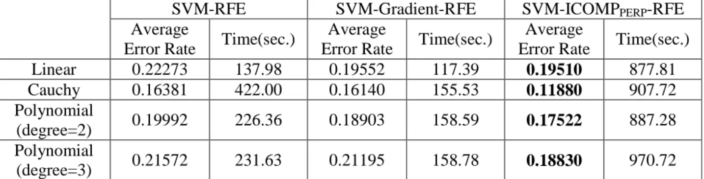
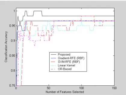
To compare three different RFE based methods; SVM-RFE, SVM-Gradient-RFE, SVM-ICOMPPERP-RFE, the ionosphere and aorta datasets are used with the same kernel functions that are used in Tables 2, 3, 6, and 7. The datasets are randomly partitioned into two cases; 20%/80% and 80%/20% as training/test sets. Tables 10 and 11 present comparisons of three RFE based methods using the ionosphere data with four different kernel functions in two different cases. The average error rate represents the misclassification error rate for the test set. The SVM-ICOMPPERF-RFE is the clear winner for most kernel functions except the linear kernel in the 80%/20% case. The best performance is obtained using the Cauchy kernel in the two cases with 88.12% and 93.28% accuracies. Tables 12 and 13 present comparisons of the three RFE based methods using the aorta data with four different kernel functions in two different cases. As shown in Tables 12 and 13, the SVM-ICOMPPERF-RFE is the best method for the polynomial kernel (degree=2) with 99.99% accuracy for the 20%/80% case, the polynomial kernel (degree=2) with 99.88% accuracy for the 80%/20% case, and the inverse multi-quadratic kernel with 100% accuracy for the 80%/20% case. Figure 4 shows line plots of error rates for the test set with the Cauchy kernel function, which gives smallest average error rates using the ionosphere data shown in Tables 10 and 11. Figure 5 shows line plots of error rates for the test set with the polynomial kernel (degree=2) and inverse multi-quadratic kernel functions, which give smallest average error rates using the aorta data shown in Tables 12, and 13. The SVM-ICOMPPERF-RFE is competitive with both SVM-RFE and SVM-Gradient-RFE as shown in Figure 4. Also,

(49)

SVM-ICOMPPERF-RFE outperforms SVM-RFE and SVM-Gradient-RFE with few variables as shown in Figure 5.

Table 10: Comparison Using Ionosphere Data with 20%/80%

SVM-RFE SVM-Gradient-RFE SVM-ICOMPPERP-RFE

Average

Error Rate Time(sec.)

Average

Linear 0.22273 137.98 0.19552 117.39 0.19510 877.81 Cauchy 0.16381 422.00 0.16140 155.53 0.11880 907.72 Polynomial (degree=2) 0.19992 226.36 0.18903 158.59 0.17522 887.28 Polynomial (degree=3) 0.21572 231.63 0.21195 158.78 0.18830 970.72

Kernel-Based Data Mining Approach with Variable Selection for Nonlinear High-Dimensional Data

University of Tennessee, Knoxville

Trace: Tennessee Research and Creative

Exchange