Hesheng Wanga)
Department of Radiation Oncology, University of Michigan, 1500 East Medical Center Drive, Ann Arbor, Michigan 48109
Yue Cao
Department of Radiation Oncology and Radiology, University of Michigan, 1500 East Medical Center Drive, Ann Arbor, Michigan 48109
(Received 10 November 2011; revised 20 April 2012; accepted for publication 9 May 2012; published 13 June 2012)
Purpose:To develop efficient algorithms for fast voxel-by-voxel quantification of tissue longitudinal relaxation time (T1) from variable flip angles magnetic resonance images (MRI) to reduce voxel-level noise without blurring tissue edges.
Methods:T1estimations regularized by total variation (TV) and quadratic penalty are developed to measure T1from fast variable flip angles MRI and to reduce voxel-level noise without decreasing the accuracy of the estimates. First, a quadratic surrogate for a log likelihood cost function of T1 estima-tion is derived based upon the majorizaestima-tion principle, and then the TV-regularized surrogate funcestima-tion is optimized by the fast iterative shrinkage thresholding algorithm. A fast optimization algorithm for the quadratically regularized T1estimation is also presented. The proposed methods are evaluated by the simulated and experimental MR data.
Results:The means of the T1values in the simulated brain data estimated by the conventional, TV-regularized, and quadratically regularized methods have less than 3% error from the true T1in both GM and WM tissues with image noise up to 9%. The relative standard deviations (SDs) of the T1 values estimated by the conventional method are more than 12% and 15% when the images have 7% and 9% noise, respectively. In comparison, the TV-regularized and quadratically regularized methods are able to suppress the relative SDs of the estimated T1 to be less than 2% and 3%, respectively, regardless of the image noise level. However, the quadratically regularized method tends to overblur the edges compared to the TV-regularized method.
Conclusions: The spatially regularized methods improve quality of T1 estimation from multiflip angles MRI. Quantification of dynamic contrast-enhanced MRI can benefit from the high quality measurement of native T1.© 2012 American Association of Physicists in Medicine.
[http://dx.doi.org/10.1118/1.4722747]
Key words: magnetic resonance imaging, variable flip angles, T1 estimation, total variation, spatial regularization, dual approach, quadratic penalty
I. INTRODUCTION
Dynamic contrast-enhanced magnetic resonance imaging (DCE-MRI) has shown its value for diagnosis of neurologi-cal disorders,1 detection of tumors, and evaluation of tissue
response to therapies.2–4 Quantification of tissue
longitudi-nal relaxation time (T1)-weighted DCE-MRI using pharma-cokinetic models requires measurement of T1 prior to con-trast injection.5Since T1values vary in tissue and tumor and
can change during and after therapy, an accurate T1 mea-surement is vital for characterization of perfusion parameters from DCE-MRI. Furthermore, quantitative tissue T1could be a distinctive metric for tissue discrimination, disease detec-tion, and therapy monitoring.6
The conventional T1 estimation is based upon either an inversion-recovery (IR) or a saturation-recovery (SR) pulse sequence. Although the methods generate accurate results, the prolonged acquisition time of these methods makes them less practical to be a part of a DCE-MRI protocol in clinical setting.7–10 The approach that is widely used in a DCE-MRI
study is to acquire gradient-echo images with variable flip
an-gles (VFA) and with one or more short TRs.11–16The scanning
time of VFA imaging can be further decreased by undersam-pling acquisition.17 Estimation of T
1 values is usually done by nonlinear least-squares fitting (NLS) of the VFA MRI,18
but also can be done by linear least-squares fitting after trans-forming intensities of MRI into a linear form with T1.9,13,19
Several authors have shown that the VFA method can achieve accuracy of the T1estimation similar to those by the IR and SR techniques for the image data having a high signal-noise ratio (SNR), which are usually accomplished by performing computation in a region of interest.14,19 However, voxel-by-voxel estimated T1values show a large amount of fluctuation due to the noise in the original images and the limited num-ber of flip angles. This poor repeatability of the T1estimation affects utilization of the T1map in voxel-based DCE quantifi-cation. In order to reduce the variation in the T1estimation, a different approach is needed. T1, as a characteristic prop-erty of the tissue, should exhibit locally spatial continuity, except at the boundary of tissue compartments. The locally spatial continuity has been successfully incorporated into the
PET reconstruction,20the B1 magnetic field correction,21and the DCE-MRI kinetic parameter quantification.22In addition, the pharmacokinetic modeling of DCE-MRI with spatial reg-ularization reduces both bias and variance of derived kinetic parameters.22
Tikhonov quadratic regularization, the most commonly used spatial regularization in image applications,20,23 has
been proposed for the T1 estimation from IR MR signals,24 and improves the SNR in the resultant T1 map. However, it is well-known that the quadratic penalty tends to oversmooth image at the boundaries of tissue compartments.25Total
vari-ation (TV), a nonquadratic regularizvari-ation, can preserve edges at tissue boundary. In this study, we proposed an efficient method by incorporating the TV regularization in the T1NLS cost function in order to reduce voxel-level noise without blur-ring edges or decreasing the accuracy in the estimates. First, we develop a quadratic surrogate function from a log like-lihood cost function according to the majorization principle, and then extend the fast iterative shrinkage thresholding al-gorithm (FISTA) for the TV-regularized (TVR) least-squares fitting of T1. To the best of our knowledge, this has not been done before. We also present an efficient quadratically reg-ularized (QR) method for T1 estimation from the VFA MR images. The proposed methods were evaluated by using syn-thesized, phantom, and clinical MR data.
II. MATERIALS AND METHODS
II.A. Nonlinear least-squares T1estimation
Based upon the Bloch equation,26a steady-state MR signal intensity (sk) acquired by a T1-weighted spoiled gradient-echo
sequence with a flip angle (FA) ofαk(k=1, 2, . . . ,NFA;NFA is the number of FAs) and a repetition time TR is given by
sk =s0 sinak(1−E) 1−Ecosak
, (1)
wheres0 is the equilibrium longitudinal magnetization, and
E=exp (−TR/T1). The T1 ands0 values at a pixel are con-ventionally estimated from measured MR signals {yk} by a
NLS fitting: (T1, s0)= NFA k=1 (yk−sk)2 subjecting to :lT1≤T1≤uT1, (2)
wherelT1 anduT1are defined by the T1 range of the tissue and utilized as a constraint to avoid unrealistic solutions and improve robustness of the computation.
It has been shown that the SNR (T1/σT1) of the T1
val-ues relates to the SNR (s0/σ) of the images by (T1/σT1)
∝(TR/T1)(s0/σ),27 indicating the noise in the original im-ages is amplified into the T1 map by the ratio of T1/TR. Therefore, the voxels with large T1 values are prone to po-tential errors. In addition, the image noise and the limited number of flip angles can cause a solution of the NLS fitting [Eq.(2)] to be trapped into a local minimum before reach-ing the real solution durreach-ing minimization.22 Although
opti-mally selecting image acquisition parameters can improve the
T1 estimation,13,14 the errors seem to persist. Therefore, we propose to incorporate prior knowledge of tissue T1 spatial continuity to improve T1estimation without compromising its accuracy.
II.B. Spatially regularized T1estimation II.B.1. TV-regularized T1estimation
TV-regularized T1estimation is to minimize the NLS cost function incorporated with TVR which is defined as
(T1, s0)=L(T1, s0)+2λT V(T1) (3) subject to :lT1≤T1≤uT1, whereL(T1, s0)= N i=1 M j=1 ln1+Ti,j1 , s0i,j (4) and TV(T1)= N i=1 M j=1
Ti1+1,j−Ti,j1 2+Ti,j1 +1−Ti,j1 2,
(5)
where (i,j) are pixel indices in a 2D space,Lis a log like-lihood function, andλis a constant that controls the relative strength of the spatial regularization.
To minimizeover the two unknown parameters (T1and
s0), we use a block alternating approach, in which T1(T1-step) ands0(s0-step) are iteratively determined by minimizing one parameter at a time while holding the other at the previously obtained value. To minimizein thes0-step, an analytic so-lution ofs0is given by s0i,j = NF A k=1 fkT1i,jyi,jk N F A k=1 fkT1i,j2, (6) where fk(T i,j
1 )=sinak(1−Ei,j)/(1−Ei,jcosak). How-ever, minimizing for T1 in the T1-step is a nontrivial problem, because is nonlinearly related to T1and the TV function [Eq.(5)] is not continuously differentiable. We de-velop a fast iterative method to minimize with respect to T1. First, we convert the log likelihoodLto a quadratic surro-gate function using the majorization principle. Then, we min-imize the TV-regularized surrogate function using an efficient algorithm based on a gradient-based dual approach.
II.B.2. Quadratic surrogate
We develop a quadratic surrogate function of the log like-lihoodLusing the majorization principle.28 The derivation is
provided in the Appendix. In brief,L(T1) is approximated by T1 −z2 for T1 near thenth iteration solution T1,n, where
z=T1,n−v/(2μ) is given in the Appendix. Then, using a matrix format, the TV-based cost function [Eq. (3)] at the (n+1)th iteration becomes
n+1=μT1−z2+2λTV(T1), (7)
where μ is the spatially variant weighting defined in the Appendix [Eq. (A3)]. As demonstrated by Eq. (A1) in the
FIG. 1. Quadratic surrogates of the likelihood term of the cost function. The likelihood function has a minimum at T1=1000. The quadratic surrogates
equate the likelihood function at T1=700 and 1300, but are above the
like-lihood curve at all other locations. The minima of the quadratic functions are converging toward the minimum of the likelihood function over iterations.
Appendix, the quadratic function is always greater thanL ex-cept at T1,n, and so can be a surrogate ofL.28 Figure1plots
an original log likelihood functionL(T1) with the true mini-mum at T1*=1000 and quadratic surrogate functions at T1,n
=700 ms and T1,n =1300 ms. At each iteration, the
mini-mum of the surrogate function moves toward the minimini-mum of
L(T1*).
II.B.3. Optimization of the TV-regularized surrogate function
The surrogate function transforms the original cost func-tion [Eq.(3)] to Eq.(7)which is a typical TV-based denoising problem with a spatially variant weightμand a spatially in-variant weightλ. Minimization of Eq.(7)still is a challenging problem due to the noncontinuously differentiable TV term. Beck29 proposes to convert the TV-based minimization to a
smooth dual problem and then solves the dual problem us-ing FISTA. Accordus-ing to the approach, two new spatially dis-tributed parameters (p,q) are introduced to convert the TV-based cost function equation (7) to a smooth dual function. The minimizer of the smooth dual function (p, q) is deter-mined by iterating (pt, qt)=(pt−1, qt−1) + 1 8(λ/μ) T Pc z− λ μ(pt−1, qt−1) , (8)
where Pc andare two projection operators,29 andtis the
iteration index. The iteration started with (p,q) being 0. After convergence of iteration(8), the T1 solution at the (n+1)th step is computed as T1,n+1=Pc z− λ μ(p, q) . (9)
The final solutions of s0and T1are sought via these inter-leaved iterations ofs0-step and T1-step.
II.B.4. Quadratic-regularized T1estimation
We also develop a method to estimate T1 with the con-ventional quadratic regularization, namely, QR, which is to minimize ¯ (T1, s0)=L(T1, s0)+βR(T1) (10) with R(T1)= 12 N i=1 M j=1 m,n(T i,j 1 −T i−m,j−n 1 )2, the
pair index (m, n) = (1,0), (–1,0), (0,1), (0,–1) denotes the coordinate offsets of the four nearest neighbors, and β is a weighting parameter for the quadratic regularization. The minimization of Eq. (10) is also done by interleaved optimizations of s0 and T1. At the T1-step, again, the log likelihood L(T1, s0) is converted to the quadratic surrogate function. As both terms in Eq.(10)become quadratic, T1 at the (n+1)th iteration is analytically solved as
T1,n+1=T1,n− 1 μ+4β ν 2+ β 2∇R(T1,n) , (11)
where matrix μandvare given in the Appendix. The final solutions of the QR method are obtained by iteratings0-step [Eq.(6)] and T1-step [Eq.(11)].
II.C. Implementation of T1estimation algorithms II.C.1. NLS T1estimation
We implement the voxel-based NLS T1estimation (Eq.(3)
withλ=0) by using the quadratic surrogate function, and re-fer it as QS-NLS method. The computation is initialized with T1=800 ms at each voxel and cycles throughs0-step [Eq.(6)] and T1-step. In T1-step, the solution at the (n+1)th iteration is analytically determined as
T1,n+1=T1,n− v
2μ. (12)
The iteration is terminated when the T1 tolerance meets |T1,n+1−T1,n|/|T1,n| ≤10−6 or the number of iterations n≥500.
II.C.2. TV-regularized T1estimation
The TVR minimization begins with the T1 estimated by the QS-NLS method. Then s0 and T1 are sought iteratively throughs0-step [Eq.(6)] and T1-step [Eq.(9)]. This iterative process is terminated when the relative change in T1<10−6 or the number of iterationsn≥250. In each T1-step, the T1 [Eq.(9)] is determined by (p,q) that result from iteration of Eq. (8). The iteration to obtain (p, q) terminates when the (p, q) tolerance is <10−6 or the iteration numbern ≥ 100. Selection ofλwill be described below.
II.C.3. Quadratic regularized T1estimation
The QR optimization is also initialized with the T1 ob-tained by the QS-NLS method, and the iterative process is terminated when T1tolerance is less than 10−6or the number of iterationsn≥250.
II.C.4. Selection of weighting parameters
The “hyperparameter”λandβ weigh the spatial regular-ization terms in the TVR and QR cost functions, respectively. Large values of the parameters can cause overweighing of the spatial regularizations, and lead to oversmoothing in the re-sulting T1map; conversely, small values can result in insuffi-cient noise reduction. To determine an appropriate weighting value ofλ(orβ), we estimated T1maps of a central slice in the simulated brain MR data with various noise levels using the TVR (or QR) method and varyingλ(or β) values on a regular grid. We selected theλ (orβ) value that minimized the averaged difference between the true and estimated T1in the central slice. We found thatλ=1 and β =0.001 were appropriate for the images with noise levels less than 7%, and λ=10 andβ =0.01 for the data with higher level noise. We applied these values to both the simulated and experimental image data for evaluation of the methods.
II.C.5. T1bound constraints
For all three methods of QS-NLS, QR, and TVR, T1bound conditions were set to belT1=50 ms anduT1=3000 ms in the simulated and phantom experiments, anduT1=6000 ms for the patient data.
II.D. Simulation studies
In order to evaluate the performance of the proposed meth-ods, we utilized the Brainweb MRI simulator to simulate VFA MRI data.30 This simulator accounts for the effects of var-ious image acquisition parameters, including partial volume averaging, noise, and sampling in Fourier domain, and inten-sity inhomogeneity in the brain tissue.31 We simulated T1-weighted MRI of a normal brain phantom using a spoiled gradient-echo pulse sequence (TR / TE of 18/10 ms, matrix size of 217 × 181 × 60, resolution of 1 × 1 × 3 mm3, and flip angles of 5◦, 10◦, 20◦, 30◦, and 40◦). Gaussian noise was added onto both real and imaginary components of MR signals in the Fourier domain to obtain noise levels of 1%, 3%, 5%, 7%, and 9% in the images. The QS-NLS, QR, and TVR methods were applied to the simulated data to estimate T1. Because of the high in-plane resolution, spatial regular-izations in both QR and TVR methods were applied in 2D images.
In order to quantitatively evaluate the methods, relative mean and relative standard deviation (rSD) are computed as the percentages of the mean and SD of the estimated T1 to the true T1 value, respectively. For the rSD calculation, the original T1 variations in WM or GM were removed. The rel-ative mean and SD measure the accuracy and stability of the methods, respectively. For statistical analysis in GM and WM, we excluded the voxels within a 2-pixel wide band from the boundary to remove the effect of blurring edges.
We also examined whether the spatially regularized meth-ods can estimate a T1map with spatial variations. We created a digital phantom that consists of the regions with (a) linear and quadratic T1 spatial variations, (b) uniform but high T1
value (1200 ms), and (c) uniform but low T1values (200 ms). MR images of the digital phantom were simulated using the Bloch equation [Eq.(1)] with five FAs (10◦, 20◦, 30◦, 50◦, and 70◦) and TR 13 ms. Random Gaussian noise was added to make the MR data have a noise level of 5%.
II.E. Experimental MRI studies
We applied the methods to experimental MR data of a EuroSpin TO5 phantom from the RIDER project,3 which was designed to evaluate the accuracy and re-peatability of MR T1 measurement. The phantom consist-ing of 18-compartments with different T1 contrasts was imaged on a 1.5 T GE scanner.3 The acquisition
pro-tocol included a 2D IR spin-echo sequence and a 3D multiple flip angles fast-spoiled gradient-echo sequence (FSPGR). The FSPGR images were acquired with seven flip angles (2◦, 5◦, 10◦, 15◦, 20◦, 25◦, and 30◦), TR/TE =6.4/1.2 ms, and a resolution of 0.55×0.55×5 mm3. Our methods were applied to the MRI data of five of the seven flip angles (5◦, 10◦, 15◦, 20◦, and 25◦) to estimate T1. The correla-tion of the compartmental means of the T1estimated from the IR and the VFA data was computed to evaluate the accuracy of the T1quantification by the proposed methods.
The methods were also tested on the brain MRI of a patient who was enrolled in a prospective DCE-MRI study of brain radiation therapy. Multiflip angle MR data were acquired on a clinical 3 T MR scanner (Ingenia, Philips Medical Systems, Best, Netherlands) with a fast spoiled gradient-echo sequence. The image parameters were TR/TE of 30 ms/2.8 ms, matrix size of 256×256×80, resolution of 1×1×2 mm3, and flip angles of 5◦, 15◦, 20◦, and 45◦. To evaluate the proposed methods, the patient was also imaged using a SR sequence with the TR of 100, 200, 500, 1000, and 2000 ms. The SR images have the same resolution and matrix as the VFA MRI. T1values were estimated voxel-by-voxel from the SR MRI by nonlinear least-square fitting.
III. RESULTS
III.A. Simulated brain
Figure2 shows estimated T1 maps of a slice in the sim-ulated brain with 5% of noise using the QS-NLS, QR, and TVR methods, as well as relative differences between the esti-mated T1and the ground truth. There are substantial amounts of noise in the regions of GM, WM, and cerebrospinal fluid (CSF) of the T1map and the difference map calculated by the QS-NLS method [Figs.2(a)and2(d)], indicating the QS-NLS method propagates or even amplifies noise from the origi-nal images onto the T1 map. In contrast, the QR and TVR methods reduce the noise in each of tissue compartments sub-stantially [Figs.2(b) and2(c) and2(e) and2(f)]. However, the relative differences between the T1 estimated by the QR method and the true values are greater at edges of tissue com-partments and in the small regions [see edge enhancement in Fig. 2(e)], indicating the effect of overblurring of the QR method. The TVR method preserves boundaries well while
FIG. 2. T1maps (top) estimated from the simulated brain dataset with five FAs and 5% noise by the QS-NLS (a), QR (b), and TVR (c). The relative differences
between the estimated T1and the ground truth are displayed in bottom row (d)–(f). The T1values range from 0 to 3000 ms in (a)–(c). The relative differences
vary from –0.2 to 0.2 in (d)–(f).
producing marked reduction of the intraregion noise in the T1 map [Figs.2(c)and2(f)].
Quantitative evaluations of the performance of the meth-ods with respect to noise on the simulated data are shown in Fig.3. The means of the T1 estimated by all the three
meth-ods show less than 3% errors from the true T1values in both GM and WM with image noise up to 9% [Figs.3(a)and3(b)]. The relative SDs of the T1estimated by the QS-NLS method increase nonlinearly with noise in the images, reaching ap-proximately 12% and 15% when there are 7% and 9% noise
FIG. 3. The relative means and standard deviations of the T1values in WM (a) and GM (b) estimated by the QS-NLS, QR, and TVR methods vs noise levels in
the original images. (c) and (d) are the relative standard deviations for WM and GM with the inner-structure T1variation (rSD at noise level 0%) removed. The
FIG. 4. T1maps of a simulated digital phantom with spatial variations of T1: homogeneous low T1values at the left and right peripheries, homogeneous high
T1values at the central region, and linearly and quadratically changed T1values from the low to high T1values in left and right, respectively. (a) The simulated
T1-weighted MRI with 5% of noise and a flip angle of 20◦; (b) the T1map without noise; (c) the T1map estimated by the QS-NLS methods; (d) the T1map
obtained by the TVR method; and (e) central-line profiles of the T1maps obtained by the QS-NLS and TVR methods compared to the true values.
[Figs. 3(c)and3(d)], respectively. In comparison, the TVR method is able to suppress the relative standard deviations of the T1values to less than 2% in both WM and GM regardless of the noise level in the image. The QR method also reduces the noise-related variations in the T1 values to be less than 3%, which is slightly greater than the one obtained by the TVR method and possibly due to the edge-blurring effect of the quadratic regularization [Figs.3(c)and3(d)].
III.B. Simulated digital phantom with spatial variations Evaluation of the performance of the spatially regularized methods on the simulated phantom with linear and quadratic spatial variations in T1 is shown in Fig.4. As expected, the T1map estimated by the QS-NLS method is very noisy, and
the central region, where the T1 value is homogeneous and high, cannot be recognized [Figs.4(c)and4(e)]. The noise in the T1map estimated by the TVR method is reduced sub-stantially, and the T1estimates clearly differentiate the homo-geneous region from the surrounding [Fig.4(d)]. Figure4(e)
plots profiles of the T1 values along a horizontal line of the phantom estimated by the QS-NLS and TVR methods. Com-pared to the true T1 values along the line, the TVR method reduces the variance in the T1 values to be 3% from 7% by the QS-NLS method.
III.C. Phantom experiments
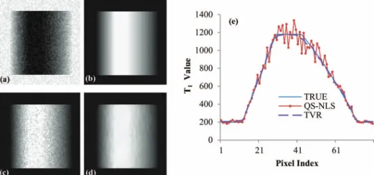
Figure5 shows T1 maps of the 18-compartment RIDER phantom estimated by the QS-NLS, QR, and TVR methods
FIG. 5. The T1maps (top) of a phantom estimated from the VFA MR data using the QS-NLS (a), QR (b), and TVR methods (c), and the relative differences
(bottom) of the estimated T1between the three VFA-based methods and the IR method (d)–(f). Gray bars denote the ranges of the T1values (top) and the relative
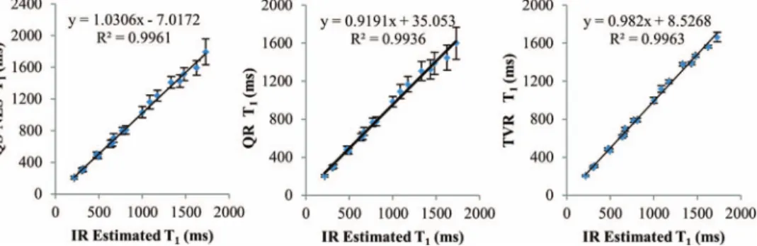
FIG. 6. Plots of the compartmental means of the estimated T1from the phantom MRI using the QS-NLS (left), QR(middle), and TVR methods (right) vs T1
values from the IR MRI data. The error bars are the standard deviations of the T1values estimated from the VFA MR data in each compartment. from the VFA MR data. Using the T1 values in each of the
compartments estimated from the IR acquisition as a refer-ence, the pixelwise relative differences between the T1values estimated by the three VFA-based methods and the reference are shown in Figs. 5(d)–5(f). Again, the TVR method pro-duces the T1map with better noise reduction and better edge preservation compared to the QS-NLS and QR methods. It is interesting to see that the QR method causes underestimation of T1values [enhancement in Fig.5(e)] around the tube edges due to overblurring of the quadratic regularization.
T1 measurements of the RIDER phantom are shown in Fig.6. There are strong linear correlations (R2 >0.99) be-tween the compartmental averaged T1values estimated from the VFA MR data using the QS-NLS, QR, and TVR meth-ods and the T1 measured from the IR MRI (a reference mea-sure). The SDs obtained by the QS-NLS method increase with the T1 values but not by the TVR method. Overall, the TVR method reduces the SDs of the T1values by a factor of 2–4 in
most of the compartments compared to the QS-NLS method. The SDs obtained by the QR method are similar to the ones obtained by the QS-NLS method due to the edge-blurring ef-fect of the QR method.
III.D. Human brain study
Figure7shows T1maps of the human brain of a patient by using the QS-NLS, QR, and TVR methods. Compared with the T1 estimated by the SR method [Figs. 7(d) and 7(h)], the T1 maps estimated by the QS-NLS method [Figs. 7(a) and7(e)] are presented with noise, which could compromise physiological parameters derived from DCE-MRI if used in DCE quantification. The T1maps obtained by the QR method [Figs. 7(b) and 7(f)] show noise reduction but also edge blurring, as evidenced by enhanced edges on the relative difference maps between by the QR and SR methods. How-ever, the TVR method [Figs.7(c)and7(g)] not only reduces
FIG. 7. T1maps of two brain slices (first and third rows) from a patient data by the QS-NLS (a) and (e); QR (b) and (f); TVR (c) and (g); and SR (d) and (h)
FIG. 8. Mean T1in the five brain ROIs on the patient images by the
QS-NLS, QR, TVR, and SR methods.
noise but also preserves structure boundaries in the T1maps, as shown in the relative difference maps between the TVR and SR methods.
The ROIs related to five different tissue structures were manually delineated on the brain images. Compared with the T1values obtained by the SR method, the mean T1in the ROIs estimated by QS-NLS, QR, and TVR methods has errors less than 5% (Fig. 8). But the QS-NLS results have greater T1 variations in the ROIs compared with the spatially regular-ized methods. Due to edge blurring, the QR method increases the standard deviation of T1 estimates in gray matter, which is also shown in the difference maps in Fig.7.
IV. DISCUSSION
In this paper, we propose spatially regularized methods to improve T1estimation based upon prior knowledge of T1 lo-cal continuity. We develop a theoretilo-cal framework for fast iterative optimization of the spatially regularized T1 quantifi-cation, including majorizing the log likelihood function to a quadratic surrogate function, converting the TV-based opti-mization to a smooth dual problem, and providing an iterative solution for T1calculation. The TVR method substantially re-duces the noise in the T1 map without image blurring or de-creasing the accuracy of the estimated T1values. Given that the quadratic surrogate only uses the T1gradient of the MR signals, our methods can be generalized to estimate T1 val-ues from MR data acquired with variable flip angles, variable TRs, or a combination of the two. Incorporating the T1 pro-duced by our methods into quantification of DCE-MRI will improve the robustness of the pharmacokinetic analysis, re-duce potential errors in local perfusion estimates, and pos-sibly improve the spatial discrimination of local changes in perfusion parameters.
The basic assumption of spatial regularization is the T1 local continuity in the tissue. To reduce the noise influence on the T1 estimation, we enforce local continuity of the T1 values while permitting rapid changes of T1 at tissue bound-aries. Our results show that the quadratic regularization, al-though reducing noise in the T1map compared to the QS-NLS method, overblurs the boundaries at the tissue compartments. In contrast, the TVR method is able to overcome the
overblur-ring problem present in the quadratic regularization method as well as reduce the noise in the T1map. A gradual T1change in a region can also be preserved by the TVR method. These two spatial regularization methods can be selected in the clinical application based upon the organ or anatomy of interest. The organs with fine tissue compartments, e.g., brain and kidney, could benefit from the TVR method. One of the potential ben-efits of the spatially regularized methods for the T1estimation is voxel-by-voxel quantification of DCE-MRI using pharma-cokinetic models, e.g., Toft model.32The noise in the T1map
can propagate into the DCE quantification and reduce repro-ducibility of derived kinetic parameters,33 which could
sub-sequently reduce the ability of these quantitative imaging pa-rameters as a biomarker for assessment of tumor and normal tissue response to therapy. The spatially regularized methods have the potential to overcome this challenge.
The total variation, as an edge-preserving regularization, has been long considered for image restoration. However, the total variation has not been widely used in the medical image field due to the complexity of the method, which involves op-timizing a noncontinuously differentiable TV function. The optimization becomes even more computation demanding when the likelihood function is a complicate nonlinear func-tion, i.e., the T1problem. A quadratic surrogate can be used to replace the nonlinear least-squares likelihood function, and therefore to simplify the optimization process. However, direct majorization of the original nonlinear least-squares cost function [Eq.(2)] to a quadratic surrogate results in a slow converging process in the T1 minimization due to the large Lipschitz constant.34 Instead, we majorize a logarithm likelihood function to a quadratic surrogate that converges much more rapidly. Furthermore, we apply the gradient-based dual approach that has been theoretically proven to have a converging rate in the order magnitude of 1/t2 (t is the iter-ation number).29 Our experiments show that the T
1 solution can converge within 100 iterations with a tolerance of 10−6.
The computation of the QS-NLS method is much faster than the conventional NLS T1 estimation,18 due to that the
QS-NLS method updates T1of all pixels in an image slice si-multaneously in each of the iterations, while the conventional NLS method minimizes the cost function voxel-by-voxel. For the computation of the simulated data on a Xeon 2.668 GHz machine and usingMATLAB2010b, it takes∼6 s to compute T1 of a 256×256 slice by the QS-NLS method, but 8 min by the conventional NLS method (using “fminsearch” in
MATLAB). Also, the differences between the T1computed by the conventional NLS and the QS-NLS method are less than 1%, indicating there is no compromise in the accuracy of the estimated T1using the QS-NLS method. With the spatial reg-ularizations, both the QR and TVR minimizations are con-verged within 100 iterations (Fig.9). Initialized with the T1 estimated by the QS-NLS method, the QR and TVR methods take additional 1.2 s and 15 s to compute the final T1 values of a 256×256 slice, respectively.
The TVR method preserves edges at tissue boundaries in a T1 map. However, the minimum size of an object or a le-sion, which can be detected by the TVR method, has not been tested and compared to the conventional methods. Like other
FIG. 9. Convergence of the QR and TVR methods from the simulated brain data with five FAs and 5% noise. The cost functions are normalized to the maximal value at the initial iteration. The two methods reach a tolerance of 1
×10–6within 100 iterations.
VFA-based methods, B1 inhomogeneity can bias the T1 esti-mated by the proposed methods because B1 inhomogeneity causes variation of flip angles. Approaches have been pro-posed to map B1 inhomogeneity.16,35 Therefore, correcting the flip angles can be performed prior to using the proposed methods.
V. CONCLUSION
T1 estimation based upon variable flip angles gradient-echo MRI has been improved by applying the prior knowl-edge of spatial continuity. Spatial regularization, either QR or TVR, can reduce random fluctuation in the T1estimates com-pared to the conventional NLS method, and thereby improve the repeatability of the pixelwise estimates. The TV regular-ization can preserve the sharp transitions between the tissue compartments better than the QR method.
ACKNOWLEDGMENTS
The authors would like to thank Dr. Edward Jackson for providing the RIDER phantom data. This work is supported in part by NIH P01 CA59827, RO1 CA132834, RO1 NS064973, and R21 CA126137.
APPENDIX: QUANDRATIC SURROGATE
The log likelihoodLnear thenth iteration solution of T1,n
at pixel (i,j) can be approximated by L(T1i,j)=ln 1+ NF A k=1 yki,j−s0i,jfk T1i,j2 ≤LT1i,j,n + NF A k=1 yki,j−s0i,jfk
T1i,j2−yki,j−s0i,jfk
T1i,j,n2 1+NF A
k=1
yki,j−s0i,jfkT1i,j,n2
.
(A1)
The right-hand side of the inequality is greater than or equal to the original L(Ti,j1 ), and therefore, can be a surro-gate for L.28 By definingdk(Ti,j
1 )=1/(1−Ei,jcos(αk)),ak
=tanαk, and bk=tanαk(cosαk−1), we havefk(T1)=ak
+bkdk(T1). Substitutingfk(T1) into the right side of Eq.(A1)
and applying the first order Taylor expansion todk(T1), Eq.(3)
in matrix format at the (n+1)th iteration of T1-step becomes
n+1=μT1−z2+2λTV(T1), (A2)
wherez=T1,n−v/(2μ),μ={μi,j}, andν={νi,j} are ma-trix formats ofμi,jandνi,jover the images computed as
μi,j = s0i,j2NFA k=1 bk∇dk Ti,j1,n2 1+NFA k=1
yki,j−s0i,jfkTi,j1,n 2 vi,j = 2s0i,j2NFA k=1b2k dk Ti,j1,n+b1 k ak− yi,jk s0i,j ∇dk Ti,j1,n 1+NFA k=1
yki,j−s0i,jfkTi,j1,n
2 ,
(A3)
where∇dk
Ti,j1,nis a gradient ofdkwith respect to T1at T1,n.
The quadratic surrogate function is always aboveLexcept at the point T1,n, and thus iteratively converges to the minimum
of L. Now, minimization of Eq.(3)becomes a conventional TV-based denoise problem.36
a)Author to whom correspondence should be addressed. Electronic mail:
1P. A. Armitage, A. J. Farrall, T. K. Carpenter, F. N. Doubal, and J. M.
Ward-law, “Use of dynamic contrast-enhanced MRI to measure subtle blood-brain barrier abnormalities,”Magn. Reson. Imaging29, 305–314 (2011).
2R. Strecker, K. Scheffler, M. Buchert, K. Mross, J. Drevs, and J.
Hen-nig, “DCE-MRI in clinical trials: Data acquisition techniques and analysis methods,” Int. J. Clin. Pharmacol. Ther.41, 603–605 (2003).
3E. F. Jackson, D. P. Barboriak, L. M. Bidaut, and C. R. Meyer, “Magnetic
resonance assessment of response to therapy: Tumor change measurement, truth data and error sources,” Transl. Oncol.2, 211–215 (2009).
4A. R. Padhani, “Dynamic contrast-enhanced MRI in clinical oncology:
Current status and future directions,”J. Magn. Reson. Imaging16, 407– 422 (2002).
5P. S. Tofts, “Modeling tracer kinetics in dynamic Gd-DTPA MR imaging,”
J. Magn. Reson. Imaging7, 91–101 (1997).
6J. Vymazal, A. Righini, R. A. Brooks, M. Canesi, C. Mariani, M. Leonardi,
and G. Pezzoli, “T1 and T2 in the brain of healthy subjects, patients with Parkinson disease, and patients with multiple system atrophy: Relation to iron content,” Radiology211, 489–495 (1999).
7N. D. Gai and J. A. Butman, “Modulated repetition time look-locker
(MORTLL): A method for rapid high resolution three-dimensional T1 mapping,”J. Magn. Reson. Imaging30, 640–648 (2009).
8S. G. Kim, X. Hu, and K. Ugurbil, “Accurate T1 determination from
in-version recovery images: Application to human brain at 4 Tesla,”Magn. Reson. Med.31, 445–449 (1994).
9P. B. Kingsley, “Methods of measuring spin-lattice (T1) relaxation times:
An annotated bibliography,”Concepts Magn. Reson.11, 243–276 (1999).
10I. R. Young, A. S. Hall, and G. M. Bydder, “The design of a multiple
in-version recovery sequence for T1 measurement,”Magn. Reson. Med.5, 99–108 (1987).
11K. A. Christensen, D. M. Grant, E. M. Schulman, and C. Walling,
“Optimal determination of relaxation times of fourier transform nu-clear magnetic resonance. Determination of spin-lattice relaxation times in chemically polarized species,” J. Phys. Chem. 78, 1971–1977 (1974).
12N. J. Pelc, “Optimization of flip angle for T1 dependent contrast in MRI,”
13E. H. Haselhoff, “Optimization of flip angle for T1 dependent contrast: A
closed form solution,”Magn. Reson. Med.38, 518–519 (1997).
14H. Z. Wang, S. J. Riederer, and J. N. Lee, “Optimizing the precision in
T1 relaxation estimation using limited flip angles,”Magn. Reson. Med.5, 399–416 (1987).
15E. K. Fram, R. J. Herfkens, G. A. Johnson, G. H. Glover, J. P. Karis, A.
Shi-makawa, T. G. Perkins, and N. J. Pelc, “Rapid calculation of T1 using vari-able flip angle gradient refocused imaging,”Magn. Reson. Imaging5, 201– 208 (1987).
16H.-L. M. Cheng and G. A. Wright, “Rapid high-resolution T1 mapping by
variable flip angles: Accurate and precise measurements in the presence of radiofrequency field inhomogeneity,”Magn. Reson. Med.55, 566–574 (2006).
17J. Velikina, A. L. Alexander, and A. A. Samsonov, “A novel approach for
T1 relaxometry using constrained reconstruction in parametric dimension,” inProc. of ISMRM 2010, 350 (2010).
18L. C. Chang, C. G. Koay, P. J. Basser, and C. Pierpaoli, “Linear
least-squares method for unbiased estimation of T1 from SPGR signals,”Magn. Reson. Med.60, 496–501 (2008).
19S. C. Deoni, B. K. Rutt, and T. M. Peters, “Rapid combined T1 and T2
map-ping using gradient recalled acquisition in the steady state,”Magn. Reson. Med.49, 515–526 (2003).
20J. H. Chang, J. M. Anderson, and J. R. Votaw, “Regularized image
recon-struction algorithms for positron emission tomography,”IEEE Trans. Med. Imaging23, 1165–1175 (2004).
21A. K. Funai, J. A. Fessler, D. T. Yeo, V. T. Olafsson, and D. C. Noll,
“Regu-larized field map estimation in MRI,”IEEE Trans. Med. Imaging27, 1484– 1494 (2008).
22B. M. Kelm, B. H. Menze, O. Nix, C. M. Zechmann, and F. A. Hamprecht,
“Estimating kinetic parameter maps from dynamic contrast-enhanced MRI using spatial prior knowledge,”IEEE Trans. Med. Imaging28, 1534–1547 (2009).
23J. W. Stayman and J. A. Fessler, “Regularization for uniform spatial
resolu-tion properties in penalized-likelihood image reconstrucresolu-tion,”IEEE Trans. Med. Imaging19, 601–615 (2000).
24F. de Pasquale, G. Sebastiani, E. Egger, L. Guidoni, A. M. Luciani, P.
Mar-zola, R. Manfredi, M. Pacilio, A. Piermattei, V. Viti, and P. Barone, “Bayesian estimation of relaxation times T(1) in MR images of irradiated Fricke-agarose gels,”Magn. Reson. Imaging18, 721–731 (2000).
25A. Borsic, B. M. Graham, A. Adler, and W. R. Lionheart, “In vivo
impedance imaging with total variation regularization,”IEEE Trans. Med. Imaging29, 44–54 (2010).
26Y. Zur, S. Stokar, and P. Bendel, “An analysis of fast imaging sequences
with steady-state transverse magnetization refocusing,” Magn. Reson. Med.6, 175–193 (1988).
27S. C. Deoni, T. M. Peters, and B. K. Rutt, “Determination of optimal angles
for variable nutation proton magnetic spin-lattice, T1, and spin-spin, T2, relaxation times measurement,”Magn. Reson. Med.51, 194–199 (2004).
28D. Böhning and B. G. Lindsay, “Monotonicity of quadratic-approximation
algorithms,”Ann. Inst. Stat. Math.40, 641–663 (1988).
29A. Beck and M. Teboulle, “A fast iterative shrinkage-thresholding
algo-rithm for linear inverse problems,” SIAM J. Imaging Sci.2, 183–202 (2009).
30K. Höhne, R. Kikinis, R. Kwan, A. Evans, and G. Pike, “An extensible MRI
simulator for post-processing evaluation,” inVisualization in Biomedical Computing(Springer, Berlin, 1996), Vol. 1131, pp. 135–140.
31R. K. Kwan, A. C. Evans, and G. B. Pike, “MRI simulation-based
evalu-ation of image-processing and classificevalu-ation methods,”IEEE Trans. Med. Imaging18, 1085–1097 (1999).
32P. S. Tofts, G. Brix, D. L. Buckley, J. L. Evelhoch, E. Henderson,
M. V. Knopp, H. B. Larsson, T. Y. Lee, N. A. Mayr, G. J. Parker, R. E. Port, J. Taylor, and R. M. Weisskoff, “Estimating kinetic parameters from dy-namic contrast-enhanced T(1)-weighted MRI of a diffusable tracer: Stan-dardized quantities and symbols,”J. Magn. Reson. Imaging10, 223–232 (1999).
33Y. Cao, D. Li, Z. Shen, and D. Normolle, “Sensitivity of quantitative
met-rics derived from DCE MRI and a pharmacokinetic model to image quality and acquisition parameters,”Acad. Radiol.17, 468–478 (2010).
34A. Beck and M. Teboulle, “Fast gradient-based algorithms for constrained
total variation image denoising and deblurring problems,”IEEE Trans. Im-age Process.18, 2419–2434 (2009).
35C. Siversson, J. Chan, C. J. Tiderius, T. C. Mamisch, V. Jellus, J.
Svens-son, and Y. J. Kim, “Effects of B(1) inhomogeneity correction for three-dimensional variable flip angle T(1) measurements in hip dGEMRIC at 3 T and 1.5 T,”Magn. Reson. Med.67, 1776–1781 (2012).
36P. L. Combettes and J. C. Pesquet, “Image restoration subject to a
to-tal variation constraint,” IEEE Trans. Image Process. 13, 1213–1222 (2004).