Marco E. G. V. Cattaneo and Andrea Wiencierz
On the implementation of LIR: the case of simple
linear regression with interval data
Technical Report Number 127, 2012
Department of Statistics
University of Munich
On the implementation of LIR:
the case of simple linear regression with interval data
Marco E. G. V. Cattaneo, Andrea Wiencierz
Department of Statistics, LMU Munich, Ludwigstraße 33, 80539 M¨unchen, Germany
Abstract
This paper considers the problem of simple linear regression with interval-censored data. That is,npairs of intervals are observed instead of thenpairs of precise values for the two variables (dependent and independent). Each of these intervals is closed but possibly unbounded, and contains the corresponding (unobserved) value of the dependent or independent variable. The goal of the regression is to describe the relationship between (the precise values of) these two variables by means of a linear function.
Likelihood-based Imprecise Regression (LIR) is a recently introduced, very general approach to regression for imprecisely observed quantities. The result of a LIR analysis is in general set-valued: it consists of all regression functions that cannot be excluded on the basis of likelihood inference. These regression functions are said to be undominated.
Since the interval data can be unbounded, a robust regression method is necessary. Hence, we consider the robust LIR method based on the minimization of the residuals’ quantiles. For this method, we prove that the set of all the intercept-slope pairs corresponding to the undominated regression functions is the union of finitely many polygons. We give an exact algorithm for determining this set (i.e., for determining the set-valued result of the robust LIR analysis), and show that it has worst-case time complexityO(n3logn). We have implemented this exact algorithm as part of the R packagelinLIR.
Keywords: simple linear regression, interval data, likelihood inference, robust regression, exact algorithm, R package
1. Introduction
Likelihood-based Imprecise Regression (LIR) is a recently introduced approach to regression for imprecisely observed quantities (see Cattaneo and Wiencierz, 2012, 2011). In this approach, it is assumed that the available data are coarse in the sense of Heitjan and Rubin (1991). That is, precise values of the quantities of interest exist, but we cannot observe them directly. Instead, we have only imprecise observations: these are subsets of the sample space, which we know to contain the precise values of the quantities of interest.
At the two extremes of the range of possible imprecise observations are the precise observations and the missing data, respectively. We have a precise observation when the imprecise observation contains a single value, which we then know to be the precise value of the quantity of interest (which in this case is thus indirectly observed). At the other extreme we have the missing data, which occur when the imprecise observation is the whole sample space, since in this case we learn nothing about the precise value of the quantity of interest.
Between these two extremes lies the whole range of possible imprecise observations, which can be any subset of the sample space. In particular, it can be argued that continuous quantities are always imprecisely observed, since no measuring device can be infinitely precise. Therefore, regression for imprecisely observed quantities is certainly an important topic in statistics. In fact, various regression methods have been proposed in several special cases (see
Email addresses:[email protected](Marco E. G. V. Cattaneo),[email protected]
for example Beaton et al., 1976; Buckley and James, 1979; Dempster and Rubin, 1983; Li and Zhang, 1998; P¨otter, 2000; Manski and Tamer, 2002; Marino and Palumbo, 2002; Gioia and Lauro, 2005; Ferson et al., 2007; Chen and Van Keilegom, 2009; Utkin and Coolen, 2011). In contrast to most of these proposals, LIR approaches the problem of regression with imprecisely observed quantities from a very general perspective.
The imprecise observations induce a likelihood function on the joint probability distributions of the random vari-ables and random sets representing the precise values and imprecise observations, respectively. The result of a LIR analysis consists of all regression functions that cannot be excluded on the basis of likelihood inference. Hence, the result of a LIR analysis is in general set-valued (set-valued results are obtained for instance also by Manski and Tamer, 2002; Marino and Palumbo, 2002; Gioia and Lauro, 2005; Vansteelandt et al., 2006; Ferson et al., 2007). The extent of the set-valued result of a LIR analysis reflects the whole uncertainty in the regression problem with imprecisely observed quantities. That is, it encompasses the statistical uncertainty due to the finite sample as well as the indeter-mination related to the fact that the quantities are only imprecisely observed (these two kinds of uncertainty in the set-valued results are discerned for example also by Manski and Tamer, 2002; Vansteelandt et al., 2006).
In the present paper we consider a robust LIR method, in which quantiles of the residuals are used to compare the possible regression functions (see Cattaneo and Wiencierz, 2012, 2011). This method is closely related to the least median (or more generally, quantile) of squares regression, which is a very robust regression method for precisely observed quantities (see for example Rousseeuw, 1984; Hampel, 1975; Hampel et al., 1986; Rousseeuw and Leroy, 1987; Maronna et al., 2006; Huber and Ronchetti, 2009). Besides being a virtue by itself, the robustness of the regression method is almost necessary when dealing with possibly unbounded imprecise observations, because an unbounded imprecise observation means that the precise value can be arbitrarily far away. In practical applications, an unbounded imprecise observation can usually be replaced by a bounded (but very wide) one: the advantage of robust methods is that they do not depend (much) on the choice of the replacing imprecise observation.
In this paper we focus on the case of simple linear regression with interval data. That is, there are two variables of interest, which are real-valued and interval-censored (i.e., the imprecise observations are possibly unbounded in-tervals). For this situation, we develop the first exact algorithm to determine the set-valued result of the robust LIR method. The first part of this algorithm is related to the first exact algorithm for least median of squares regression, proposed by Steele and Steiger (1986) (see also Rousseeuw and Leroy, 1987, Chapter 5), which was also the basis of many other developments (see for example Souvaine and Steele, 1987; Edelsbrunner and Souvaine, 1990; Stromberg, 1993; Hawkins, 1993; Carrizosa and Plastria, 1995; Watson, 1998; Bernholt, 2005; Mount et al., 2007).
The paper is organized as follows. In the next section, we briefly present the robust LIR method in the framework of simple linear regression with interval data. Section 3 contains the main results of the paper, expressed as two theorems, whose proofs are in the appendix. These results give us an exact algorithm for the robust LIR method. The computational complexity of the algorithm is then studied in Subsection 3.3. We have implemented the algorithm as part of an R package, which is briefly introduced in Subsection 3.4, and applied to an illustrative example in Section 4. The final section is devoted to conclusions and directions for further research.
2. LIR in the case of simple linear regression with interval data
In the case of simple linear regression, the relation between two real-valued variables,XandY, shall be described by means of a linear function. Hence, the set of all possible regression functions isF :={fa,b:a,b ∈R}, where the functionsfa,b:R→Rare defined byfa,b(x)=a+b xfor allx∈R. We consider here the case of imprecisely observed quantities, and in particular of interval data. That is, instead of directly observing the realizations of the variablesX
andY, we can only observe the realizations of the extended real-valued variables X, X, Y, and Y, which are the
endpoints of the interval data [X,X] and [Y,Y]. Throughout the paper, [w,w] denotes the closed interval consisting of all real numberswsuch thatw≤w≤w. This notation is used for allw,w ∈R, so that the interval [w,w] is empty whenw>w, and does not contain its endpoints when these are infinite.
2.1. The probability model
The only assumption about the joint distribution of the six random variablesX,Y,X,X,Y, andYis the following:
for someε∈[0,1/2[. That is, apart for the choice ofε, the probability model is fully nonparametric: it is only assumed
that the (possibly unbounded) rectangle [X,X]×[Y,Y] contains the pair (X,Y) with probability at least 1−ε. In other words, an imprecise observation may not cover the precise data point with probability at mostε. The usual choice ofεis 0 (see for instance Heitjan and Rubin, 1991), but sometimes it can be useful to allow the imprecise data to be incorrect with a positive probability, andε ∈ ]0,1/2[ is then an upper bound on this probability. Apart from this
assumption, there is no restriction on the set of possible distributions of the precise and imprecise data. In particular, nothing is assumed about the joint distribution of the quantities of interest,XandY.
The relation betweenXandY shall be described by a linear function f ∈ F. For each f ∈ F, the quality of the description depends on the marginal distribution of the (absolute) residual
Rf :=|Y−f(X)|.
The more this distribution is concentrated near 0, the better is the description of the relation betweenXandY. In the robust LIR method that we consider in this paper, the concentration near 0 of the distribution of the residualRf is
evaluated by its median, or more generally by itsp-quantile, withp∈]ε,1−ε[. The closer to 0 thep-quantile is, the better f describes the relation betweenXandY. In particular, the best description of the relation of interest is a linear function for which thep-quantile of the residual’s distribution is minimal.
Assuming for simplicity that the p-quantiles of the distribution ofRf are unique for all f ∈ F, and that there is
a unique f0 ∈ F such that the corresponding p-quantileq0 ∈R≥0is minimal, we can characterize geometrically the
best description f0as follows. For eachf ∈ F and eachq∈R≥0, let
Bf,q:=n(x,y)∈R2:|y−f(x)| ≤qo
be the closed band of (vertical) width 2q around the graph of f. Then Bf0,q0 is the thinnest band of the form Bf,q
containing (X,Y) with probability at least p. This is in particular the case whenY has for eachx∈Ra conditional distribution givenX =xthat is strictly unimodal and symmetric around f0(x) (see also Tasche, 2003). That is, in the
linear modelY =a0+b0X+E, the best description in the above sense is f0= fa0,b0, when the conditional distribution
of the error termE|X=xis strictly unimodal and symmetric (around 0) for allx∈R(e.g., when the error termEis independent ofXand normally distributed with mean 0).
2.2. The LIR analysis
Let the nonempty (possibly unbounded) rectangles [x1,x1]×[y1,y1], . . . ,[xn,xn]×[yn,yn]⊆R2benindependent realizations of the random set [X,X]×[Y,Y]. The LIR analysis consists in using likelihood inference to identify a set of plausible regression functions. The imprecise data induce a (nonparametric) likelihood function on the set of all joint probability distributions (of X, Y, X, X, Y, and Y) satisfying condition (1). For each f ∈ F, let Cf
be the likelihood-based confidence region with cutoff pointβ for the p-quantile of the distribution of Rf, where
β∈
(max{p,1−p}+ε)n,1. That is,C
f consists of all possible values of thep-quantile of the distribution ofRf, for
all probability distributions whose likelihood exceedsβtimes the maximum of the likelihood function (see Cattaneo and Wiencierz, 2012, for more details).
In order to obtain an explicit formula for the confidence regionsCf, we define
k:=max k∈ {1, . . . ,n−1}:k<(p−ε)n and p−ε k k 1−p+ε n−k !n−k ≤ β nn ∪ {0} , k:=min k∈ {1, . . . ,n−1}:k>(p+ε)n and p+ε k k 1−p−ε n−k !n−k ≤ β nn ∪ {n} .
Clearly, the two integerskandkdepend onε,p,n, andβ, and satisfy
0≤k<(p−ε)n≤p n≤(p+ε)n<k≤n.
Moreover, whenε, p, andn are fixed,k andkare an increasing and a decreasing function of β, respectively, and in particular, ifβis sufficiently large, thenk = ⌈(p−ε)n⌉ −1 (i.e., the largest integer smaller than (p−ε)n) and k=⌊(p+ε)n⌋+1 (i.e., the smallest integer larger than (p+ε)n).
Now, for each function f ∈ F and each imprecise observation [xi,xi]×[yi,yi], we define the lower and upper (absolute) residuals rf,i:= min (x,y)∈[xi,xi]×[yi,yi] |y−f(x)|, rf,i:= sup (x,y)∈[xi,xi]×[yi,yi] |y−f(x)|.
Obviously,rf,i≤rf,i, andrf,i∈R≥0, whilerf,i∈R≥0. In particular,rf,i= +∞if and only if either the linear functionf
is not constant and the rectangle [xi,xi]×[yi,yi] is unbounded, or f is constant and the interval [yi,yi] is unbounded.
As usual in statistics,rf,(i) andrf,(i) denote then theith smallest lower and upper residuals, respectively. That is,
rf,(1) ≤ · · · ≤ rf,(n) are the ordered lower residuals and rf,(1) ≤ · · · ≤ rf,(n) are the ordered upper residuals. Then
Corollary 2 of Cattaneo and Wiencierz (2012) implies that
Cf =[rf,(k+1),rf,(k)]
for all f ∈ F. That is, the likelihood-based confidence region Cf ⊆ R≥0 is a nonempty closed interval, which is bounded if and only if either fis not constant and there are at leastkbounded imprecise observations, or f is constant and there are at leastkimprecise observations [xi,xi]×[yi,yi] such that the interval [yi,yi] is bounded.
It is important to note that in general the intervalCf is proper (i.e., it contains more than one value), even whenβ is so large thatk=⌈(p−ε)n⌉ −1 andk=⌊(p+ε)n⌋+1. In this case,Cf represents the maximum likelihood estimate of the p-quantile of the distribution of Rf, which in general is not a single value because the data are imprecise
and quantiles of a distribution are not necessarily unique. For example, ifn is even, ε = 0, and p = 1/2, then ⌈(p−ε)n⌉=⌊(p+ε)n⌋=n/2, and thus the maximum likelihood estimate of the p-quantile (i.e., the median) of the
distribution ofRf is [rf,(n/2),rf,(n/2+1)].
Hence, for each linear function f ∈ F, we have an interval estimateCf for the p-quantile of the distribution of
the (absolute) residualRf. We would like to select the regression function f ∈ F by minimizing this estimate, but
comparing the intervalsCf gives us only a partial order onF. The linear functions f ∈ F that are minimal according
to this partial order are said to be undominated. That is, f is undominated if and only if there is no f′∈ F such that rf′,(k) <rf,(k+1). In order to simplify the description of the undominated functions, define
qLRM :=inf f∈Frf,(k)
(the nameqLRMshall be clarified in Subsection 3.1). The set of all undominated regression functions
U:={f ∈ F :rf,(k+1)≤qLRM}
is the result of the robust LIR method considered in this paper. It represents the whole uncertainty about the linear function that best describes the relation betweenXandY, including the statistical uncertainty due to the finite sample as well as the indetermination related to the fact that the quantities are only imprecisely observed.
3. An exact algorithm for LIR
We now present an exact algorithm for determining the result of the robust LIR analysis described in Section 2. That is, an exact algorithm for calculating the set U of all undominated regression functions, given n nonempty (possibly unbounded) rectangles [x1,x1]×[y1,y1], . . . ,[xn,xn]×[yn,yn] ⊆ R2 and the two integers k andk with 0≤k<k≤n. The algorithm consists of two parts: in the first one, we determine the boundqLRM, which is then used
in the second part to identify the setU. As we will see, the computational complexity of the algorithm isO(n3logn).
We have implemented this exact algorithm as part of an R package, which we will briefly introduce at the end of the present section.
3.1. Part 1: Determining the bound qLRM
LetDbe the set of alli∈ {1, . . . ,n}such that the rectangle [xi,xi]×[yi,yi] is bounded. Then defineB:={0}if
there are less thankbounded imprecise observations (i.e., if|D|<k, where|D|denotes the cardinality of the setD), and B:= (y i−yj xi−xj : (i,j)∈ D2 and xi>xj and yi>yj ) ∪ (y i−yj xi−xj : (i,j)∈ D2 and xi>xj and yi<yj ) ∪ (y i−yj xi−xj : (i,j)∈ D2 and xi>xj and yi<yj ) ∪ (y i−yj xi−xj : (i,j)∈ D2 and xi>xj and yi>yj ) ∪ {0}
otherwise (i.e., if|D| ≥k). The central ideas of the first part of the algorithm are that in order to obtainqLRMit suffices
to consider the linear functions fa,bwith slopeb∈ B, and that for each slopebthe intercepta∈Rminimizingrfa,b,(k)
can be easily calculated, since the problem becomes one-dimensional. These ideas are formalized in the following theorem, but first we need some additional definitions. For eachb∈Rand eachi∈ {1, . . . ,n}, define
zb,i= yi−b xi if b<0, yi if b=0, yi−b xi if b>0, zb,i= yi−b xi if b<0, yi if b=0, yi−b xi if b>0.
For eachb∈Rand each j∈ {1, . . . ,n}, as usual,zb,(j)andzb,(j) denote then the jth smallest value among thezb,iand
among thezb,i, respectively. Furthermore, for eachb ∈ Rand each j ∈ {1, . . . ,n−k+1}, letzb,[j] denote thekth
smallest value among thezb,isuch thatzb,i≥zb,(j).
Theorem 1. If there are less than k imprecise observations[xi,xi]×[yi,yi]such that the interval[yi,yi]is bounded,
then
qLRM = +∞,
{f ∈ F :rf,(k)=qLRM}=F.
Otherwise (i.e., when there are at least k imprecise observations[xi,xi]×[yi,yi] such that the interval [yi,yi] is
bounded), qLRM =12 min (b,j)∈B×{1,...,n−k+1}(zb,[j]−zb,(j)), {f ∈ F :rf,(k) =qLRM} ⊇ fa′,b′ : (b′,j′)∈ arg min (b,j)∈B×{1,...,n−k+1} (zb,[j]−zb,(j)) and a′=12(zb′,(j′)+zb′,[j′]) ,
where the set on the left-hand side is infinite when the inclusion is strict. However, the inclusion is an equality when the following condition is satisfied: if there is a pair(i,j)∈ D2such that x
i=xjandmax{yi,yj}−min{yi,yj}=2qLRM,
then i,j and the two intervals[yi,yi]and[yj,yj]are nested (i.e., either[yi,yi]⊆[yj,yj], or[yj,yj]⊆[yi,yi]).
For each linear function f ∈ F, we have a likelihood-based confidence region [rf,(k+1),rf,(k)] for thep-quantile of
the residual’s distribution. Hence, the functions f ∈ F minimizingrf,(k)can be interpreted as the results of a minimax
approach to our regression problem: they are called Likelihood-based Region Minimax (LRM) regression functions (see Cattaneo, 2007). For these functions, the upper endpoint of the interval estimate of thep-quantile of the residual’s distribution isqLRM, which explains its name.
Theorem 1 implies in particular that an LRM regression function always exists, though it is not necessarily unique. When it is unique, it is denoted byfLRM. In this case,BfLRM,qLRMis the thinnest band of the formBf,qcontaining at least
kimprecise observations, for all f ∈ F and allq∈R≥0. More generally, if there are at leastkimprecise observations [xi,xi]×[yi,yi] such that the interval [yi,yi] is bounded, then 2qLRM is the (vertical) width of the thinnest bands of the
formBf,qcontaining at leastkimprecise observations (there can be more than one such bands, but only finitely many
when the condition at the end of Theorem 1 is satisfied).
If all interval data are degenerate: xi = xi andyi = yi for all i ∈ {1, . . . ,n} (i.e., the imprecise data are in
fact precise), then the LRM regression functions correspond to the least quantile of squares (or absolute residuals) regression functions f ∈ F minimizing the (square of the)kth smallest absolute residualrf,(k)=rf,(k)(see Rousseeuw
and Leroy, 1987). That is, the LRM regression functions can be interpreted as the results of a generalization of the least quantile of squares regression to the case of imprecise data. The first part of our algorithm corresponds to a generalization (to the case of general quantiles and imprecise data) of the first exact algorithm for least median of squares regression, proposed by Steele and Steiger (1986) (see also Rousseeuw and Leroy, 1987, Chapter 5).
The key result behind Theorem 1 is that (when the condition at the end of the theorem is satisfied and there are at leastkimprecise observations [xi,xi]×[yi,yi] such that the interval [yi,yi] is bounded) ifBf′,q′is one of the thinnest
bands of the formBf,q containing at leastkimprecise observations, then the union of these imprecise observations touches one of the two borders ofBf′,q′in at least two different points. This is a simple consequence of general results
by Cheney (1982, Chapters 1 and 2), as suggested by Stromberg (1993). From this property it follows that one of the two borders ofBf′,q′(which obviously have the same slope as f′) is the line determined by two points on the borders
of the imprecise observations contained inBf′,q′. Hence, either the slope of f′is 0, or it is determined by two vertices
of a pair of bounded imprecise observations contained inBf′,q′. The setBconsists of all the possible slopes that can
be obtained in this way: they are at most 4n2+1. For each possible slopeb∈ B, finding the thinnest bands of the formBfa,b,q containing at leastkimprecise observations (for all a ∈ Rand allq ∈ R≥0) corresponds to finding the
shortest intervals (of the form [a−q,a+q]) containing at leastkof thenintervals [zb,1,zb,1], . . . ,[zb,n,zb,n]. This is a
finite problem: it suffices to consider the intervals [zb,(j),zb,[j]] with j∈ {1, . . . ,n−k+1}.
Therefore, Theorem 1 gives us an algorithm for determining the boundqLRM, by reducing the minimization of
rf,(k)on the infinite setF to a minimization problem on the finite setB × {1, . . . ,n−k+1}. Moreover, when there are
finitely many LRM regression functions, Theorem 1 gives us an algorithm for finding all of them. An explicit formula for the set of all LRM regression functions in the general case (i.e., also when the condition at the end of the theorem is not satisfied) can be easily obtained, but requires several case distinctions and goes beyond the scope of the present paper.
3.2. Part 2: Identifying the setU
After having determined the boundqLRM, in the second part of the algorithm we identify the setUof all
undomi-nated regression functions (i.e., the result of the robust LIR analysis described in Section 2).
Theorem 2. U= fa,b:b∈R and a∈ n−k [ j=1 [zb,(k+j)−qLRM,zb,(j)+qLRM] .
A linear function f ∈ F is undominated if and only ifrf,(k+1) ≤ qLRM. That is, if and only if the band Bf,qLRM
intersects at leastk+1 imprecise observations. For each possible slope b ∈ R, finding all the bands of the form Bfa,b,qLRM intersecting at leastk+1 imprecise observations (for alla∈R) corresponds to finding all the intervals of the
form [a−qLRM,a+qLRM] intersecting at leastk+1 of thenintervals [zb,1,zb,1], . . . ,[zb,n,zb,n]. For eachb ∈Rand each nonempty setI ⊆ {1, . . . ,n}, the interval [a−qLRM,a+qLRM] (witha ∈R) intersects all the intervals [zb,i,zb,i] withi∈ Iif and only ifa∈[maxi∈Izb,i−qLRM,mini∈Izb,i+qLRM]. Therefore,
U= fa,b :b∈R and a∈ [ I⊆{1,...,n}:|I|=k+1 max i∈I zb,i −qLRM,min i∈I zb,i+qLRM .
Theorem 2 gives a simpler expression forU, in which the number of intervals in the union is reduced fromk+n1to n−k.
Hence, Theorem 2 gives us an algorithm for identifying, for each possible slopeb ∈ R, the set of all intercepts a∈Rsuch that the linear function fa,bis undominated. This suffices for most practical purposes, but Theorem 2 also
enables us to precisely describe as union of finitely many (possibly unbounded) polygons the set
U′:=n(a,b)∈R2: fa,b∈ Uo
of all the intercept-slope pairs corresponding to the undominated regression functions. More precisely,U′is a subset of the planeR2bounded by finitely many line segments and half-lines. However,U′is not necessarily convex nor connected, and if there are imprecise observations [xi,xi]×[yi,yi] such that the interval [xi,xi] is unbounded and
[yi,yi],R, thenU′is not even necessarily closed.
Consider first the case with no imprecise observations [xi,xi]×[yi,yi] such that the interval [xi,xi] is unbounded
and [yi,yi], R. In this case, for eachi ∈ {1, . . . ,n}, the functionb 7→ zb,ionRis either continuous and piecewise linear, or constant equal−∞, while the functionb 7→zb,ionRis either continuous and piecewise linear, or constant equal+∞. Therefore, for each j ∈ {1, . . . ,n−k}, the functionb 7→ zb,(k+j)−qLRM onRis either continuous and piecewise linear, or constant equal−∞, while the functionb7→zb,(j)+qLRM onRis either continuous and piecewise linear, or constant equal+∞. Thus, Theorem 2 implies thatU′is a closed subset of the plane
R2bounded by finitely many line segments and half-lines. That is,U′is the union of finitely many (possibly unbounded) polygons (see for example Alexandrov, 2005, Subsection 1.1.1).
If [xi,xi]×[yi,yi] is an imprecise observation such that the interval [xi,xi] is unbounded and [yi,yi],R, then at least one of the two functionsb 7→ zb,iandb 7→ zb,ionRhas a discontinuity atb =0. Therefore, in this case, the functionsb 7→zb,(k+j)−qLRMandb7→zb,(j)+qLRMonR(with j∈ {1, . . . ,n−k}) can be discontinuous atb=0. As a consequence, Theorem 2 implies thatU′is a subset of the plane
R2bounded by finitely many line segments and half-lines, butU′is not necessarily closed. However, the two partsU′∩(
R× {0}) andU′∩(R×R,0) are relatively
closed inR× {0}andR×R,0, respectively. 3.3. Computational complexity
The algorithm consisting of the two parts presented in Subsections 3.1 and 3.2 is the first exact algorithm to determine the result of the robust LIR analysis in the case of simple linear regression with interval data. It has worst-case time complexityO(n3logn), exactly as the first exact algorithm for least median of squares regression (see Steele and Steiger, 1986).
In the first part of the algorithm, described in Subsection 3.1, for each possible slopeb∈ B, we must determine the pair (zb,(j),zb,[j]) (with j∈ {1, . . . ,n−k+1}) such that the differencezb,[j]−zb,(j)is minimal. We can do this as follows:
after having calculated the valueszb,1, . . . ,zb,n andzb,1, . . . ,zb,n, we sort the two lists, obtainingzb,i1, . . . ,zb,in (with
zb,ij =zb,(j)) andzb,(1), . . . ,zb,(n). Then, for each jfrom 1 ton−k+1, we retrieve the pair consisting of the jth entry
(i.e.,zb,ij) in the first list and of thekth entry in the second one, and after that we remove the valuezb,ijfrom the second
list. In this way, the pairs of values that we have retrieved include all the pairs (zb,(j),zb,[j]) with j∈ {1, . . . ,n−k+1}
(and possibly some irrelevant additional pairs with larger differences, if some of thezb,i are equal), and we did not have to calculate a new list ofzb,ifor each jin order to determinezb,[j].
Hence, for each possible slope, we have to calculate and sort two lists of lengthn, which can be done in time O(nlogn), and then for each j ∈ {1, . . . ,n−k+1}, we have to search and remove a value from the second list, which can be done in timeO(logn) using balanced trees (see for example Knuth, 1998, Subsection 6.2.3). Therefore, since there are at most 4n2+1 possible slopes, the worst-case time complexity of the first part of the algorithm is O(n3logn).
In the second part of the algorithm, described in Subsection 3.2, for a given slopeb∈R, we must determine the pairs (zb,(k+j),zb,(j)) for all j ∈ {1, . . . ,n−k}. This can be done in timeO(n logn), since it suffices to calculate and
sort the two listszb,1, . . . ,zb,nandzb,1, . . . ,zb,n, and then, for each jfrom 1 ton−k, retrieve the pair consisting of the
(k+j)th entry in the first list and of the jth entry in the second one.
For example, if we want to graphically represent the setU′of all the intercept-slope pairs (a,b)∈
R2 correspond-ing to the undominated regression functions fa,b, then it suffices to consider a finite number of possible values for the
slopeb, resulting in a worst-case time complexity ofO(n logn) for the second part of the algorithm. However, if the goal is to precisely describe the setU′as union of finitely many (possibly unbounded) polygons, then the (worst-case) number of valuesb ∈ Rthat must be considered depends onn. In this case, it suffices to consider all valuesb ∈R
such that some of the 2ngraphs of the functionsb 7→ zb,iandb 7→ zb,icross each other, and five additional values for the slopeb. More precisely, these additional values are 0, a positive and a negative value sufficiently near 0 (in order to clarify what happens in the limitsb ↓ 0 andb ↑ 0), and finally a positive and a negative value sufficiently far from 0 (in order to clarify what happens in the limitsb ↑ +∞andb ↓ −∞). Therefore, the worst-case number of valuesb ∈ Rthat must be considered is 222n+5, and so the worst-case time complexity of the second part of the algorithm isO(n3logn), when the goal is to precisely describe the setU′ as union of finitely many (possibly unbounded) polygons.
Altogether, the worst-case time complexity of the whole algorithm for the robust LIR analysis is thusO(n3logn).
3.4. R package
We have implemented the presented algorithm in R (R Development Core Team, 2012) as part of a package called linLIR(Wiencierz, 2012). This R package is created to implement LIR methods for the case of linear regression with interval data. The available version of thelinLIRpackage includes a function to create a particular data object for interval-valued observations (idf.create), the functions.linlirto perform the LIR analysis for two variables out of the data object, and some associated methods for the generic functionsprint,summary, andplot. Both parts of the algorithm are incorporated in thes.linlirfunction. The correspondingplotmethod provides tools to visualize the results including, e.g., the setU′. Moreover, the R package contains two example data sets including the one analyzed in Section 4. The current version of the R package is not optimized for speed, yet it provides a ready-to-use first implementation of the robust LIR method for linear regression with interval data.
4. Example
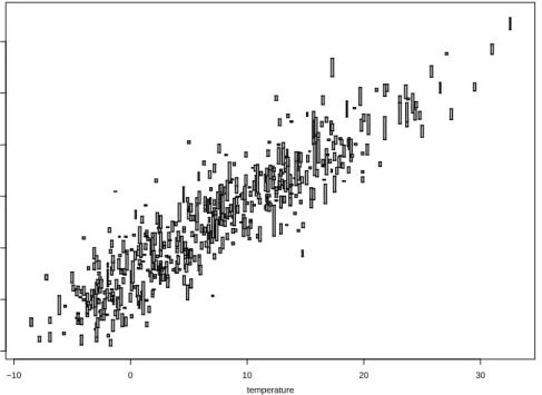
In many practical settings data are only available with limited precision. Consider, for example, the situation where it shall be analyzed how particulate matter concentration in the air varies with surface temperature. To investigate this relation, data is collected. The temperature is measured by means of a thermometer at randomly selected points in time during a certain period. From the instructions manual of the thermometer it is known that the measurement accuracy is, e.g.,±0.05◦C, which translates the measured values into small intervals of width 0.1◦C. Furthermore, there is a nearby measuring station for air pollution where four times a day recent data about particulate matter concentration is published, each time referring to a period of six hours. Among the published data there are the minimum and the maximum concentration measured during the corresponding period. Thus, for each temperature measurement at a particular time, the available information is that the corresponding particulate matter concentration lies in the interval of values measured during the corresponding six-hour period. That is, also this variable is only imprecisely observed. The data set to be analyzed in the described situation might be similar to the simulated data set shown in Figure 1. This data set consists of 514 interval-valued observations of two variables. The data of the independent variable each have the same amount of imprecision, because the indetermination stems from the measurement accuracy of the thermometer determining the width of the intervals. By contrast, the width of the interval-valued observations of the dependent variable is given by the range of measured values during a fixed period and therefore varies a lot.
In the remainder of this section, we use the simulated data set to illustrate the implementation of the robust LIR method in thelinLIRpackage. We here assume that the data are correct in the sense that the observed rectangles contain the correct precise values with probability one, i.e., we assumeε = 0. If we had concerns about the data quality, e.g., if it were likely that there have been some mistakes in recording the data, a positiveεcould be considered. This would lead to a more imprecise result of the LIR analysis, reflecting the fact that there is additional uncertainty in the data.
Before conducting the LIR analysis, we have to choose the quantilepto be considered and the cutoffpointβ. It can be proved that the LIR analysis yields the most robust results when the median of the distribution of the residuals is considered, as for the least quantile of squares regression (see also Rousseeuw and Leroy, 1987, Chapter 3). Therefore, we setp=0.5. Furthermore, we chooseβ=0.5 as cutoffpoint for the likelihood-based confidence regionsCf with f ∈ F. The confidence regions Cf are asymptotically (conservative) confidence intervals of level Fχ2(−2 logβ),
whereFχ2 is the cumulative distribution function of the chi-square distribution with 1 degree of freedom. Thus, the
choice ofβ = 0.5 implies an asymptotic lower bound for the confidence level ofCf of 76.1% (see Cattaneo and Wiencierz, 2012). Thes.linlirfunction of the R package provides also the finite-sample level of the (conservative)
−10 0 10 20 30 0 10 20 30 40 50 60 temperature par
ticulate matter concentr
ation ● ● ● ● ● ● ● ● ● ● ● ● ● ● ● ● ● ● ● ● ● ● ● ● ● ● ● ● ● ● ● ● ● ● ● ● ● ● ● ● ● ● ● ● ● ● ● ● ● ● ● ● ●● ●● ● ● ● ●● ● ● ● ● ● ● ● ●● ●● ●● ●● ●● ●● ● ● ● ● ● ● ● ● ● ● ● ● ● ● ● ● ● ● ● ● ● ● ● ● ● ● ● ● ● ● ● ● ● ● ● ● ● ● ● ● ● ● ● ● ● ● ● ● ● ● ● ● ● ● ● ● ● ● ● ● ● ● ● ● ● ● ● ● ● ● ● ● ●● ●● ● ● ● ● ● ● ● ● ● ● ● ● ● ● ● ● ● ● ● ● ● ● ● ● ● ● ● ● ● ● ● ● ● ● ● ● ● ● ● ● ● ● ● ● ● ● ● ● ●● ●● ● ● ● ● ●● ●● ● ● ● ● ● ● ● ● ● ● ● ● ● ● ● ● ● ● ● ● ● ● ● ● ● ● ● ● ● ● ● ● ● ● ● ● ● ● ● ● ● ● ● ● ●● ●● ● ● ● ● ● ● ● ● ● ● ● ● ● ● ● ● ● ● ● ● ● ● ● ● ● ● ● ● ● ● ● ● ●● ●●●● ●● ● ● ● ● ● ● ● ● ● ● ● ● ● ● ● ● ● ● ● ● ● ● ● ● ● ● ● ● ● ● ● ● ●● ●● ● ● ● ● ● ● ● ● ● ● ● ● ● ● ● ● ● ● ● ● ● ● ● ● ● ● ● ● ●● ●● ● ● ● ● ● ● ● ● ● ● ● ● ● ● ● ● ● ● ● ● ● ● ● ● ● ● ● ● ● ● ● ●●● ●● ●● ●● ● ● ● ● ● ● ● ● ● ● ● ● ● ● ● ● ● ● ● ● ●● ●● ● ● ● ● ● ● ● ● ● ● ● ● ●● ●● ● ● ● ● ● ● ● ● ● ● ● ● ● ● ● ● ● ● ● ●● ● ● ● ● ● ● ● ●● ●● ● ● ● ● ● ● ● ● ●● ●● ● ● ● ●● ● ● ● ● ● ● ● ● ● ● ● ● ● ● ● ● ● ● ● ●● ●● ● ● ● ● ● ● ● ● ●● ●● ●● ●● ● ● ● ● ● ● ● ●●●●● ● ● ● ● ● ● ● ● ●● ●● ● ● ● ● ● ● ● ● ● ● ● ● ● ● ● ● ● ● ● ● ● ● ● ● ● ● ● ● ● ● ● ● ● ● ● ● ● ● ● ● ● ● ● ● ● ● ● ● ● ● ● ● ● ● ● ● ● ● ● ● ●● ●● ● ● ● ● ●● ●● ● ● ● ● ● ● ● ● ● ● ● ● ● ● ● ● ● ● ● ● ● ● ● ● ● ● ● ● ● ● ● ● ●● ●● ● ● ● ● ● ● ● ● ● ● ● ● ● ● ● ● ● ● ● ● ● ● ● ●● ● ● ● ● ● ● ● ● ● ● ● ● ● ● ● ● ● ● ● ● ● ● ● ● ● ● ● ●● ●● ● ● ● ● ●● ●● ● ● ● ● ● ● ● ● ● ● ● ● ●● ●● ● ● ● ● ● ● ● ● ●● ●● ● ● ● ● ● ● ● ● ● ● ● ● ● ● ● ● ● ● ● ● ● ● ● ● ● ● ● ● ● ● ● ● ● ● ● ● ● ● ● ● ● ● ● ● ● ● ● ● ● ● ● ● ●● ●● ● ● ● ● ● ● ● ● ● ● ● ● ● ● ● ● ● ● ● ● ● ● ● ● ●● ●● ● ● ● ● ● ● ● ● ● ● ● ●●●●● ● ● ● ● ● ● ● ● ● ● ● ● ● ● ● ●● ● ● ● ● ● ● ● ● ● ● ● ●● ●● ● ● ● ● ● ● ● ● ● ● ● ● ● ● ● ● ● ● ● ● ● ● ● ● ● ● ● ● ● ● ● ● ● ● ● ● ● ● ● ● ● ● ● ● ● ● ● ● ● ● ● ● ● ● ● ● ● ● ● ● ● ● ● ● ● ● ● ● ● ● ● ● ● ● ● ● ● ● ● ● ● ● ● ● ● ● ● ● ● ● ● ● ● ● ● ● ● ● ● ● ● ● ● ● ● ● ● ● ● ● ● ● ● ● ● ● ● ● ● ● ●● ●● ● ● ● ● ● ● ● ● ● ● ● ● ● ● ● ● ● ● ● ● ● ● ● ● ● ● ● ● ● ● ● ● ● ● ● ● ● ● ● ● ● ● ● ● ●● ●●●● ●● ● ● ● ● ● ● ● ● ● ● ● ● ● ● ● ● ● ● ● ● ● ● ● ● ● ● ● ● ● ● ● ● ● ● ● ●● ● ● ● ● ● ● ● ● ● ● ● ● ● ● ● ● ● ● ● ● ● ● ● ● ● ● ● ● ● ● ● ● ● ● ● ● ● ● ● ● ● ● ● ● ● ● ● ● ● ● ● ● ● ● ● ●● ●●● ● ● ●● ● ● ● ● ● ● ● ● ● ● ● ●● ●● ● ● ● ● ● ● ● ● ● ● ● ● ● ● ● ● ● ● ● ● ● ● ● ● ● ● ● ● ● ● ● ● ●● ●● ●● ●● ● ● ● ● ● ● ● ● ● ● ● ● ● ● ● ● ● ● ● ● ● ● ● ● ● ● ● ● ● ● ● ●● ● ● ● ● ● ● ● ●● ●● ● ● ● ● ● ● ● ● ●● ●● ● ● ● ● ● ● ● ● ● ● ● ● ● ● ● ● ● ● ● ● ● ● ● ● ● ● ● ● ● ● ● ● ● ● ● ● ●● ●● ● ● ● ● ● ● ● ● ● ● ● ● ●● ●● ● ● ● ● ●● ●● ● ● ● ● ●● ●● ● ● ● ● ● ● ● ● ● ● ● ● ● ● ● ●● ● ● ● ● ● ● ● ● ● ● ● ● ● ● ● ● ● ● ● ● ● ● ● ● ● ● ● ● ● ● ● ● ● ● ● ● ● ● ● ● ● ● ● ● ● ● ● ● ● ● ● ● ● ● ● ● ● ● ● ● ● ● ● ● ● ● ● ● ● ● ● ● ● ● ● ● ● ● ● ● ● ● ● ● ● ● ● ● ● ● ● ● ● ● ● ● ● ● ● ● ● ● ● ● ● ● ● ● ● ● ● ● ● ● ● ● ● ● ● ●● ●● ● ● ● ● ●● ●● ● ● ● ● ● ● ● ● ● ● ● ● ● ● ● ●● ● ● ● ● ● ● ● ● ● ● ● ● ● ● ● ● ● ● ● ● ● ● ● ●● ●● ●● ●● ●● ●● ● ● ● ● ● ● ● ● ● ● ● ● ● ● ● ● ● ● ● ● ● ● ● ● ● ● ● ● ● ● ● ● ●● ●● ●● ●● ● ● ● ●●● ●● ● ● ● ● ● ● ● ● ● ● ● ● ● ● ● ● ● ● ● ● ● ● ● ● ●● ●● ●● ●● ●● ●● ●● ●● ● ● ● ● ● ● ● ●● ● ● ● ● ● ● ● ● ● ● ● ● ● ● ● ●● ●● ● ● ● ● ● ● ● ● ● ● ● ● ● ● ● ● ● ● ● ● ● ● ● ● ● ● ● ● ● ● ● ● ● ● ● ● ● ● ● ● ● ● ● ● ● ● ● ● ● ● ● ● ● ● ● ● ●● ●● ● ● ● ● ● ● ● ● ● ● ● ● ● ● ● ● ● ● ● ● ● ● ● ● ● ● ● ● ● ● ● ● ● ● ● ● ● ● ● ● ● ● ● ● ● ● ● ● ● ● ● ● ● ● ● ● ● ● ● ● ● ● ● ● ● ● ● ● ●● ●● ●● ●● ● ● ● ● ● ● ● ● ● ● ● ● ●● ●● ● ● ● ● ● ● ● ● ● ● ● ● ● ● ● ● ● ● ● ● ● ● ● ● ● ● ● ● ● ● ● ● ● ● ● ● ● ● ● ● ● ● ● ● ● ● ● ● ● ● ● ● ●● ●● ● ● ● ● ● ● ● ● ●● ●● ● ● ● ● ● ● ● ● ● ● ● ● ● ● ● ● ● ● ● ●● ● ● ● ● ● ● ● ● ● ● ● ●● ●● ● ● ● ● ● ● ● ● ● ● ● ● ● ● ● ● ● ● ● ● ● ● ● ● ● ● ● ● ● ● ● ● ● ● ● ● ● ● ● ● ● ● ● ● ● ● ● ● ● ● ● ● ● ● ● ● ● ● ● ● ● ● ● ● ● ● ● ● ● ● ● ● ● ● ● ● ● ● ● ● ● ● ● ● ● ● ● ● ● ● ● ● ● ● ● ● ● ● ● ● ● ● ● ● ● ● ● ● ●● ●● ● ● ● ● ● ● ● ● ● ● ● ● ● ● ● ●
Figure 1: Simulated data set with 514 interval-valued observations of two variables, labeled as temperature and particulate matter concentration.
confidence intervals, which can be derived by simple combinatorial arguments. In the present situation the exact minimum confidence level is 78.28%. A thorough exhibition of the argumentation, however, would go beyond the scope of the present paper.
Using the functions.linlirof the R packagelinLIRwith the above choices, we obtain the following results: Estimated parameters of the function f.lrm:
intercept of f.lrm: 15.61906
slope of f.lrm: 1.293166
Ranges of parameter values of the undominated functions: intercept of f in [6.537292,23.53457]
slope of f in [0.6552,2.156] Number of observations: 514 LIR settings:
p: 0.5 beta: 0.5 epsilon: 0 k.l: 243 k.u: 271
confidence level of each confidence interval: 78.28 %
We find that there is a unique function that minimizes the right endpoint of the confidence interval for the median of the residuals’ distribution, namelyfLRM(x)=15.62+1.29x. This function corresponds to the line at the center of the
thinnest closed band containing at leastk=271 of the given imprecise observations. The setUof all undominated regression functions covers lines with intercepts between 6.54 and 23.53 and slopes ranging from 0.66 to 2.16. The closed bandsBf,qLRM of (vertical) width 2qLRM =8.18 around the lines f ∈ Ueach intersect at leastk+1 = 244
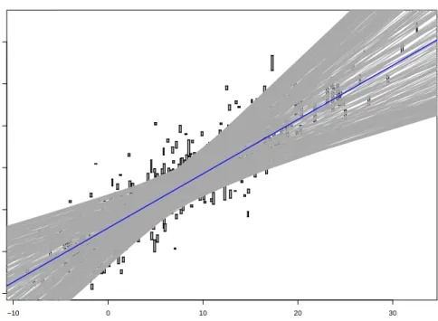
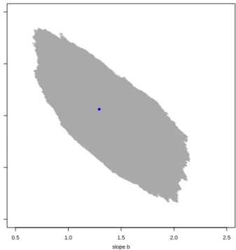
imprecise observations. To visualize the results, we can use the plot method associated with the output of the functions.linlir. One can choose between plotting a random selection of functions out of the setU, or the entire setU′. Figure 2 shows 500 randomly selected undominated regression lines, which clearly indicate that there is a positive correlation between the investigated variables. The set of all intercept-slope combinations corresponding to the undominated regression lines is displayed in Figure 3, providing a nice illustration of the complex shape of this
−10 0 10 20 30 0 10 20 30 40 50 60 temperature par
ticulate matter concentr
ation ● ● ● ● ● ● ● ● ● ● ● ● ● ● ● ● ● ● ● ● ● ● ● ● ● ● ● ● ● ● ● ● ● ● ● ● ● ● ● ● ● ● ● ● ● ● ● ● ● ● ● ● ●● ●● ● ● ● ●● ● ● ● ● ● ● ● ●● ●● ●● ●● ●● ●● ● ● ● ● ● ● ● ● ● ● ● ● ● ● ● ● ● ● ● ● ● ● ● ● ● ● ● ● ● ● ● ● ● ● ● ● ● ● ● ● ● ● ● ● ● ● ● ● ● ● ● ● ● ● ● ● ● ● ● ● ● ● ● ● ● ● ● ● ● ● ● ● ●● ●● ● ● ● ● ● ● ● ● ● ● ● ● ● ● ● ● ● ● ● ● ● ● ● ● ● ● ● ● ● ● ● ● ● ● ● ● ● ● ● ● ● ● ● ● ● ● ● ● ●● ●● ● ● ● ● ●● ●● ● ● ● ● ● ● ● ● ● ● ● ● ● ● ● ● ● ● ● ● ● ● ● ● ● ● ● ● ● ● ● ● ● ● ● ● ● ● ● ● ● ● ● ● ●● ●● ● ● ● ● ● ● ● ● ● ● ● ● ● ● ● ● ● ● ● ● ● ● ● ● ● ● ● ● ● ● ● ● ●● ●●●● ●● ● ● ● ● ● ● ● ● ● ● ● ● ● ● ● ● ● ● ● ● ● ● ● ● ● ● ● ● ● ● ● ● ●● ●● ● ● ● ● ● ● ● ● ● ● ● ● ● ● ● ● ● ● ● ● ● ● ● ● ● ● ● ● ●● ●● ● ● ● ● ● ● ● ● ● ● ● ● ● ● ● ● ● ● ● ● ● ● ● ● ● ● ● ● ● ● ● ●●● ●● ●● ●● ● ● ● ● ● ● ● ● ● ● ● ● ● ● ● ● ● ● ● ● ●● ●● ● ● ● ● ● ● ● ● ● ● ● ● ●● ●● ● ● ● ● ● ● ● ● ● ● ● ● ● ● ● ● ● ● ● ●● ● ● ● ● ● ● ● ●● ●● ● ● ● ● ● ● ● ● ●● ●● ● ● ● ●● ● ● ● ● ● ● ● ● ● ● ● ● ● ● ● ● ● ● ● ●● ●● ● ● ● ● ● ● ● ● ●● ●● ●● ●● ● ● ● ● ● ● ● ●●●●● ● ● ● ● ● ● ● ● ●● ●● ● ● ● ● ● ● ● ● ● ● ● ● ● ● ● ● ● ● ● ● ● ● ● ● ● ● ● ● ● ● ● ● ● ● ● ● ● ● ● ● ● ● ● ● ● ● ● ● ● ● ● ● ● ● ● ● ● ● ● ● ●● ●● ● ● ● ● ●● ●● ● ● ● ● ● ● ● ● ● ● ● ● ● ● ● ● ● ● ● ● ● ● ● ● ● ● ● ● ● ● ● ● ●● ●● ● ● ● ● ● ● ● ● ● ● ● ● ● ● ● ● ● ● ● ● ● ● ● ●● ● ● ● ● ● ● ● ● ● ● ● ● ● ● ● ● ● ● ● ● ● ● ● ● ● ● ● ●● ●● ● ● ● ● ●● ●● ● ● ● ● ● ● ● ● ● ● ● ● ●● ●● ● ● ● ● ● ● ● ● ●● ●● ● ● ● ● ● ● ● ● ● ● ● ● ● ● ● ● ● ● ● ● ● ● ● ● ● ● ● ● ● ● ● ● ● ● ● ● ● ● ● ● ● ● ● ● ● ● ● ● ● ● ● ● ●● ●● ● ● ● ● ● ● ● ● ● ● ● ● ● ● ● ● ● ● ● ● ● ● ● ● ●● ●● ● ● ● ● ● ● ● ● ● ● ● ●●●●● ● ● ● ● ● ● ● ● ● ● ● ● ● ● ● ●● ● ● ● ● ● ● ● ● ● ● ● ●● ●● ● ● ● ● ● ● ● ● ● ● ● ● ● ● ● ● ● ● ● ● ● ● ● ● ● ● ● ● ● ● ● ● ● ● ● ● ● ● ● ● ● ● ● ● ● ● ● ● ● ● ● ● ● ● ● ● ● ● ● ● ● ● ● ● ● ● ● ● ● ● ● ● ● ● ● ● ● ● ● ● ● ● ● ● ● ● ● ● ● ● ● ● ● ● ● ● ● ● ● ● ● ● ● ● ● ● ● ● ● ● ● ● ● ● ● ● ● ● ● ● ●● ●● ● ● ● ● ● ● ● ● ● ● ● ● ● ● ● ● ● ● ● ● ● ● ● ● ● ● ● ● ● ● ● ● ● ● ● ● ● ● ● ● ● ● ● ● ●● ●●●● ●● ● ● ● ● ● ● ● ● ● ● ● ● ● ● ● ● ● ● ● ● ● ● ● ● ● ● ● ● ● ● ● ● ● ● ● ●● ● ● ● ● ● ● ● ● ● ● ● ● ● ● ● ● ● ● ● ● ● ● ● ● ● ● ● ● ● ● ● ● ● ● ● ● ● ● ● ● ● ● ● ● ● ● ● ● ● ● ● ● ● ● ● ●● ●●● ● ● ●● ● ● ● ● ● ● ● ● ● ● ● ●● ●● ● ● ● ● ● ● ● ● ● ● ● ● ● ● ● ● ● ● ● ● ● ● ● ● ● ● ● ● ● ● ● ● ●● ●● ●● ●● ● ● ● ● ● ● ● ● ● ● ● ● ● ● ● ● ● ● ● ● ● ● ● ● ● ● ● ● ● ● ● ●● ● ● ● ● ● ● ● ●● ●● ● ● ● ● ● ● ● ● ●● ●● ● ● ● ● ● ● ● ● ● ● ● ● ● ● ● ● ● ● ● ● ● ● ● ● ● ● ● ● ● ● ● ● ● ● ● ● ●● ●● ● ● ● ● ● ● ● ● ● ● ● ● ●● ●● ● ● ● ● ●● ●● ● ● ● ● ●● ●● ● ● ● ● ● ● ● ● ● ● ● ● ● ● ● ●● ● ● ● ● ● ● ● ● ● ● ● ● ● ● ● ● ● ● ● ● ● ● ● ● ● ● ● ● ● ● ● ● ● ● ● ● ● ● ● ● ● ● ● ● ● ● ● ● ● ● ● ● ● ● ● ● ● ● ● ● ● ● ● ● ● ● ● ● ● ● ● ● ● ● ● ● ● ● ● ● ● ● ● ● ● ● ● ● ● ● ● ● ● ● ● ● ● ● ● ● ● ● ● ● ● ● ● ● ● ● ● ● ● ● ● ● ● ● ● ●● ●● ● ● ● ● ●● ●● ● ● ● ● ● ● ● ● ● ● ● ● ● ● ● ●● ● ● ● ● ● ● ● ● ● ● ● ● ● ● ● ● ● ● ● ● ● ● ● ●● ●● ●● ●● ●● ●● ● ● ● ● ● ● ● ● ● ● ● ● ● ● ● ● ● ● ● ● ● ● ● ● ● ● ● ● ● ● ● ● ●● ●● ●● ●● ● ● ● ●●● ●● ● ● ● ● ● ● ● ● ● ● ● ● ● ● ● ● ● ● ● ● ● ● ● ● ●● ●● ●● ●● ●● ●● ●● ●● ● ● ● ● ● ● ● ●● ● ● ● ● ● ● ● ● ● ● ● ● ● ● ● ●● ●● ● ● ● ● ● ● ● ● ● ● ● ● ● ● ● ● ● ● ● ● ● ● ● ● ● ● ● ● ● ● ● ● ● ● ● ● ● ● ● ● ● ● ● ● ● ● ● ● ● ● ● ● ● ● ● ● ●● ●● ● ● ● ● ● ● ● ● ● ● ● ● ● ● ● ● ● ● ● ● ● ● ● ● ● ● ● ● ● ● ● ● ● ● ● ● ● ● ● ● ● ● ● ● ● ● ● ● ● ● ● ● ● ● ● ● ● ● ● ● ● ● ● ● ● ● ● ● ●● ●● ●● ●● ● ● ● ● ● ● ● ● ● ● ● ● ●● ●● ● ● ● ● ● ● ● ● ● ● ● ● ● ● ● ● ● ● ● ● ● ● ● ● ● ● ● ● ● ● ● ● ● ● ● ● ● ● ● ● ● ● ● ● ● ● ● ● ● ● ● ● ●● ●● ● ● ● ● ● ● ● ● ●● ●● ● ● ● ● ● ● ● ● ● ● ● ● ● ● ● ● ● ● ● ●● ● ● ● ● ● ● ● ● ● ● ● ●● ●● ● ● ● ● ● ● ● ● ● ● ● ● ● ● ● ● ● ● ● ● ● ● ● ● ● ● ● ● ● ● ● ● ● ● ● ● ● ● ● ● ● ● ● ● ● ● ● ● ● ● ● ● ● ● ● ● ● ● ● ● ● ● ● ● ● ● ● ● ● ● ● ● ● ● ● ● ● ● ● ● ● ● ● ● ● ● ● ● ● ● ● ● ● ● ● ● ● ● ● ● ● ● ● ● ● ● ● ● ●● ●● ● ● ● ● ● ● ● ● ● ● ● ● ● ● ● ●
Figure 2: Selection of 500 undominated regression lines out of the setU. The functionfLRMis highlighted.
set. In both cases, the line fLRMor the corresponding intercept-slope combination (bLRM,aLRM) is highlighted.
As we already mentioned at the end of Section 3, the current version of the functions.linlirhas not been optimized for speed yet. The computations for the present analysis took roughly 70 minutes on a desktop computer, most of the time is needed for the first part of the algorithm, whereqLRMis determined.
5. Conclusion
In this paper, we considered the LIR approach to regression for imprecisely observed quantities (see Cattaneo and Wiencierz, 2012, 2011). The result of a LIR analysis is in general set-valued: it consists of all regression functions that cannot be excluded on the basis of likelihood inference. These regression functions are said to be undominated. In this paper, we considered in particular the robust LIR method based on the residuals’ quantiles, in the special case of simple linear regression with interval data. For this situation, we proved that the set of all the intercept-slope pairs corresponding to the undominated regression functions is the union of finitely many polygons, and we gave an exact algorithm for determining this set (i.e., for determining the set-valued result of the robust LIR method).
We have implemented this exact algorithm as part of the R packagelinLIR(Wiencierz, 2012). In the present paper, we illustrated the implementation of the robust LIR method in thelinLIRpackage by means of an example. Furthermore, we showed that the algorithm has worst-case time complexityO(n3logn). In fact, the first part of the
algorithm is related to the first exact algorithm for least median of squares regression, which has the same (asymptotic) worst-case time complexity (see Steele and Steiger, 1986; Rousseeuw and Leroy, 1987). This algorithm for least median of squares regression was then improved (see for example Souvaine and Steele, 1987; Edelsbrunner and Souvaine, 1990; Carrizosa and Plastria, 1995; Mount et al., 2007) and extended to multiple linear regression (see for instance Stromberg, 1993; Hawkins, 1993; Watson, 1998; Bernholt, 2005). In future work, we intend to do the same with the algorithm for the robust LIR method. Moreover, this algorithm can also be generalized to imprecise data other than intervals.
0.5 1.0 1.5 2.0 2.5 5 10 15 20 25 slope b intercept a ●
Figure 3: SetU′of all intercept-slope pairs corresponding to the undominated regression functions. The point (b
LRM,aLRM) is highlighted.
Appendix A. Proofs
The following lemma gives us a method for writing the union of allnkpossible intersections ofkout ofnintervals as the union ofn−k+1 other intervals. It will be used in the proof of Theorem 2, but can be useful also for other problems, such as constructing an explicit formula for the set of all LRM regression functions in the general case (i.e., also when the condition at the end of Theorem 1 is not satisfied).
Lemma 1. If w1, . . . ,wn,w1, . . . ,wn∈Rwith wi≤wifor all i∈ {1, . . . ,n}, then for each k∈ {1, . . . ,n},
[ I⊆{1,...,n}:|I|=k \ i∈I [wi,wi]= n [ j=k [w(j),w(j−k+1)],
where for each j ∈ {1, . . . ,n}, as usual, w(j) and w(j) denote the jth smallest value among w1, . . . ,wn and among
w1, . . . ,wn, respectively.
This lemma can be proved as follows. Assume without loss of generality thatw1 ≤ · · · ≤ wn(i.e.,w(j) =wj),
and for allj,j′∈ {1, . . . ,n}with j≤ j′, letw
j:j′denote the jth smallest value amongw1, . . . ,wj′(hence, in particular,
w(j)=wj:n). Then, for each setI ⊆ {1, . . . ,n}with cardinality|I|=k,
\
i∈I
[wi,wi]=
max
i∈I wi,mini∈I wi
=wmaxI,min
i∈I wi
⊆[wmaxI,wmaxI−k+1:maxI],
and obviously maxI ∈ {k, . . . ,n}. Furthermore, for each j∈ {k, . . . ,n}, there are at most j−kindicesi∈ {1, . . . ,n}
such thatwi<w(j−k+1), and thus there is a setIj ⊆ {1, . . . ,j}with cardinality|Ij|=ksuch thatwi ≥w(j−k+1)for all
i∈ Ij. Therefore, n [ j=k [w(j),w(j−k+1)]⊆ n [ j=k " max i∈Ij wi,min i∈Ij wi # = n [ j=k \ i∈Ij [wi,wi]⊆ [ I⊆{1,...,n}:|I|=k \ i∈I [wi,wi] ⊆ [ I⊆{1,...,n}:|I|=k
[wmaxI,wmaxI−k+1:maxI]=
n
[
j=k
Hence, in order to complete the proof of the lemma, it suffices to show that the first and last unions ofn−k+1 intervals in the above expression are equal. To this goal, we first show that for each j∈ {k, . . . ,n−1},
[wj,wj−k+1:j]∪[wj+1,wj+1−k+1:j+1]=[wj,w(j−k+1)]∪[wj+1,wj+1−k+1:j+1]. (A.1)
Sincew(j−k+1)≤wj−k+1:jalways holds, (A.1) could be wrong only ifw(j−k+1)<wj−k+1:j, which can be the case only if
there is an indexi∈ {j+1, . . . ,n}such thatwi≤w(j−k+1), but then
wj≤wj+1≤wi≤wi≤w(j−k+1)<wj−k+1:j≤wj+1−k+1:j+1,
and thus both unions in (A.1) are equal to the interval [wj,wj+1−k+1:j+1]. Therefore, using (A.1) for each jfromkto
n−1, we obtain n [ j=k [wj,wj−k+1:j]= n−1 [ j=k [wj,w(j−k+1)] ∪[wn,wn−k+1:n]= n−1 [ j=k [w(j),w(j−k+1)] ∪[w(n),w(n−k+1)]= n [ j=k [w(j),w(j−k+1)].
Appendix A.1. Proof of Theorem 1
As noted in Subsection 2.2, for each linear function f ∈ F, we haverf,(k) < +∞if and only if either f is not
constant and there are at leastkbounded imprecise observations, or f is constant and there are at leastkimprecise observations [xi,xi]×[yi,yi] such that the interval [yi,yi] is bounded. Therefore, if there are less thankimprecise
observations [xi,xi]×[yi,yi] such that the interval [yi,yi] is bounded, thenrf,(k) = +∞for all f ∈ F, which proves
the first part of the theorem. Otherwise, if there are at leastkimprecise observations [xi,xi]×[yi,yi] such that the
interval [yi,yi] is bounded, as we assume from now on, thenrf,(k) < +∞at least for the constant functions f ∈ F,
which impliesqLRM<+∞.
For each function fa,b∈ F and each imprecise observation [xi,xi]×[yi,yi],
zb,i= inf (x,y)∈[xi,xi]×[yi,yi] (y−b x), (A.2) zb,i= sup (x,y)∈[xi,xi]×[yi,yi] (y−b x), (A.3) and therefore rfa,b,i=max sup (x,y)∈[xi,xi]×[yi,yi] (y−a−b x), sup (x,y)∈[xi,xi]×[yi,yi] (a+b x−y) =
max{zb,i−a,a−zb,i}. Hence, thekth smallest upper residual of fa,bis
rfa,b,(k)= min
I⊆{1,...,n}:|I|=kmaxi∈I max
{zb,i−a,a−zb,i}= min
I⊆{1,...,n}:|I|=kmax
max i∈I zb,i −a,a−min i∈I zb,i .
Now, for each setI ⊆ {1, . . . ,n}with cardinality|I|=k, there is a j∈ {1, . . . ,n−k+1}such thatzb,(j) =mini∈Izb,i, and in this case, sincezb,i≥zb,(j)for alli∈ I, the smallest possible value of maxi∈Izb,iiszb,[j]. Thus we obtain
rfa,b,(k)= min
j∈{1,...,n−k+1}max
{zb,[j]−a,a−zb,(j)}.
Clearly, for eachb∈Randj∈ {1, . . . ,n−k+1}such that the interval [zb,(j),zb,[j]] is bounded, the maximum ofzb,[j]−a
anda−zb,(j)is uniquely minimized by the interval centera=1/2(zb,(j)+zb,[j]). This implies
qLRM= inf (a,b)∈R2 rfa,b,(k) = 1 2(b,j)∈ inf R×{1,...,n−k+1}(zb,[j] −zb,(j)), {f ∈ F :rf,(k)=qLRM}= fa′,b′: (b′,j′)∈ arg min (b,j)∈R×{1,...,n−k+1} (zb,[j]−zb,(j)) and a′=12(zb′,(j′)+zb′,[j′]) .
Therefore, in order to complete the proof of the theorem, it suffices to show that the set M:= b′: (a′,b′)∈arg min (a,b)∈R2 rfa,b,(k) = b′: (b′,j′)∈ arg min (b,j)∈R×{1,...,n−k+1} (zb,[j]−zb,(j))
intersectsB(i.e.,M ∩ B,∅), thatMis infinite whenM*B, and thatM ⊆ Bwhen the condition at the end of the theorem is satisfied.
For each setI ⊆ {1, . . . ,n}with cardinality|I|=k, letgIbe the function (a,b)7→maxi∈Irfa,b,ionR
2. Then, for
alla,b∈R,
rfa,b,(k)= min
I⊆{1,...,n}:|I|=kgI(a,b).
LetSbe the (nonempty) set of all setsI ⊆ {1, . . . ,n}with cardinality|I| =ksuch that inf(a,b)∈R2gI(a,b) =qLRM. Then, defining for eachI ∈ S,
MI:= b′: (a′,b′)∈arg min (a,b)∈R2 gI(a,b) , we obtainM=S
I∈SMI. Hence, in order to complete the proof of the theorem, it suffices to show for eachI ∈ S, that the setMIintersects B(i.e.,MI∩ B , ∅), thatMIis infinite whenMI * B, and thatMI ⊆ B when the condition at the end of the theorem is satisfied.
Let I ∈ S, and consider first the case with I * D. In this case, there is an i ∈ Isuch that the rectangle [xi,xi]×[yi,yi] is unbounded, and sinceqLRM < +∞, there area,b ∈ Rsuch thatrfa,b,i < +∞. As noted in
Sub-section 2.2, this implies that the interval [yi,yi] is unbounded, and thenrfa,b,i <+∞if and only if the function fa,bis
constant. That is,gI(a,b)<+∞if and only ifb=0, and thereforeMI={0} ⊆ B.
Consider now the case withI ⊆ D(i.e., the rectangle [xi,xi]×[yi,yi] is bounded for alli∈ I), which implies in
particular|D| ≥k. In this case,
gI(a,b)=max
i∈I (x,y)∈{maxxi,xi}×{yi,yi}
|y−a−b x|
for alla,b ∈ R, since for a bounded imprecise observation [xi,xi]×[yi,yi], the upper residualrfa,b,i is the
max-imum of the four residuals corresponding to the vertices of the rectangle [xi,xi]×[yi,yi]. The Existence
Theo-rem of Cheney (1982, page 20) implies then that arg min(a,b)∈R2gI(a,b) is not empty (i.e., MI , ∅). Let thus (a′,b′)∈arg min
(a,b)∈R2gI(a,b) (hence,b
′∈ MI). From the Characterization Theorem of Cheney (1982, page 35) it follows that there are (x,y),(x′,y′)∈S
i∈I{xi,xi} × {yi,yi}such that eitherx,x′and both points (x,y),(x′,y′) lie on
the graph of one of the two functions fa′+q
LRM,b′ and fa′−qLRM,b′, orx= x
′and the point (x,y) lies on the graph of the function fa′+q
LRM,b′, while the point (x
′,y′) lies on the graph of the functionf
a′−q
LRM,b′.
All the (bounded) rectangles [xi,xi]×[yi,yi] withi ∈ Iare contained in the closed band Bfa′,b′,qLRM of (vertical)
width 2qLRM around the graph of the functionfa′,b′, and the points (x,y),(x′,y′) are vertices of these rectangles lying
on the border of the bandBfa′,b′,qLRM. Ifx, x
′, then (x,y) and (x′,y′) lie on the same border ofB
fa′,b′,qLRM, and thus
determine its slope
b′= y−y ′ x−x′.
It can be easily checked that the setBcontains all the slopes that can be obtained in this way by the vertices of the bounded imprecise observations [xi,xi]×[yi,yi]. Therefore, ifx,x′, thenb′∈ B.
Assume now thatb′<B. In order to complete the proof of the theorem, it suffices to show that in this case the set
MIis infinite and intersectsB, and that the condition at the end of the theorem cannot be satisfied. The assumption b′<Bimpliesx=x′. Hence, the points (x,y) and (x′,y′) are two vertices of two (bounded) rectangles [xi,xi]×[yi,yi]
and [xj,xj]×[yj,yj] (withi,j∈ I), and lie on the upper and on the lower borders of the bandBfa′,b′,qLRM, respectively.
If eitherx, xiandx′, xj, or x,xiandx′, xj, then the intervals [xi,xi] and [xj,xj] are proper (i.e., they contain
more than one value) and extend on the same side of x = x′, but this would implyb′ = 0 ∈ B, because the two rectangles [xi,xi]×[yi,yi] and [xj,xj]×[yj,yj] must be contained in the bandBfa′,b′,qLRM. Therefore,xi=xjorxi=xj,
and max{yi,yj} −min{yi,yj}=y−y′=2qLRM. That is, one of the two pairs (i,j),(j,i)∈ I2⊆ D2satisfies the premise
of the condition at the end of the theorem. Now, if [yi,yi]⊆[yj,yj], then the interval [xj,xj] must be degenerate (i.e.,
the bandBfa′,b′,qLRM. Analogously, if [yj,yj]⊆[yi,yi], thenxi =xi. Hence, if the two intervals [yi,yi] and [yj,yj] are
nested, then one of the two pairs (i,i),(j,j)∈ D2satisfies the premise of the condition at the end of the theorem. So
this condition is contradicted by at least one of the four pairs (i,j),(j,i),(i,i),(j,j)∈ D2.
In order to complete the proof of the theorem, it remains to show that the setMIis infinite and intersectsB. We have thatb∈ MIif and only if there is ana∈Rsuch that the closed bandBfa,b,qLRM of (vertical) width 2qLRM around
the graph of the function fa,bcontains the 4kvertices of the rectangles [xi,xi]×[yi,yi] withi∈ I. For eachb ∈R, since the two vertices (x,y),(x′,y′) satisfyx=x′andy−y′ =2q
LRM, the band Bfa,b,qLRM can contain the 4kvertices
only ifa=ab :=1/2(y′+y)−b x(i.e., only if the midpoint of (x,y) and (x′,y′) is contained in the graph of the linear
function fa,b). Now, for each vertex (x′′,y′′), the set of allb ∈Rsuch that the bandBfab,b,qLRM contains (x
′′,y′′) is the closed interval Bx′′,y′′ = " y′−y′′ x′−x′′, y−y′′ x−x′′ # if x′′<x=x′, R if x′′=x=x′, " y′′−y x′′−x, y′′−y′ x′′−x′ # if x′′>x=x′,
where the second case is implied by the fact thatBx′′,y′′ is not empty (sinceb′∈ MI⊆ Bx′′,y′′), while in the other two
cases the endpoints ofBx′′,y′′are the slopesbdetermined by the pairs of points (x,y),(x′′,y′′) or (x′,y′),(x′′,y′′) lying
on the same border ofBfab,b,qLRM. Therefore, MI= \ i∈I \ (x′′,y′′)∈{x i,xi}×{yi,yi} Bx′′,y′′
is a (nonempty) closed interval, which is eitherRor it is bounded. WhenMI=R, obviously it is infinite and intersects
B. Otherwise,MIis a bounded interval whose endpoints are elements ofB, since they are slopesbdetermined by a pair of vertices lying on the same border ofBfab,b,qLRM. Hence, also in this caseMIintersectsBand is infinite, since
b′<Bis an interior point of the intervalMI.
Appendix A.2. Proof of Theorem 2
For each function fa,b∈ F and each imprecise observation [xi,xi]×[yi,yi], using (A.2) and (A.3), we obtain that
rfa,b,i≤qLRM if and only if the set
y−f
a,b(x) : (x,y)∈[xi,xi]×[yi,yi] =[zb,i−a,zb,i−a]
intersects the interval [−qLRM,qLRM]. That is, rfa,b,i ≤ qLRM if and only ifa ∈ [zb,i−qLRM,zb,i+qLRM]. Hence,
rfa,b,(k+1)≤qLRM if and only if there is a setI ⊆ {1, . . . ,n}such that|I|=k+1 anda ∈[zb,i−qLRM,zb,i+qLRM] for
alli∈ I. That is, using Lemma 1 withk=k+1, we obtain thatrfa,b,(k+1)≤qLRMif and only ifalies in the set
[ I⊆{1,...,n}:|I|=k+1 \ i∈I [zb,i−qLRM,zb,i+qLRM]= n [ j=k+1 [zb,(j)−qLRM,zb,(j−k)+qLRM]= n−k [ j=1 [zb,(k+j)−qLRM,zb,(j)+qLRM]. Therefore, U={fa,b∈ F :rfa,b,(k+1)≤qLRM}= fa,b:b∈R anda∈ n−k [ j=1 [zb,(k+j)−qLRM,zb,(j)+qLRM] . References
Alexandrov, A.D., 2005. Convex Polyhedra. Springer.
Beaton, A.E., Rubin, D.B., Barone, J.L., 1976. The acceptability of regression solutions: Another look at computational accuracy. J. Am. Stat. Assoc. 71, 158–168.
Bernholt, T., 2005. Computing the least median of squares estimator in timeO(nd), in: Gervasi, O., Gavrilova, M.L., Kumar, V., Lagan`a, A., Lee,