Validation Document Delft3D-FLOW

(1)

Report

a software system for 3D flow simulations

(2)

(3)

H. Gerritsen, E.D. de Goede, F.W. Platzek,

M. Genseberger, J.A.Th.M. van Kester and R.E. Uittenbogaard

Report

X0356, M3470

(4)

(5)

Client:

Title: Validation Document Delft3D-FLOW; a software system for 3D flow simulations

Abstract:

This report is the validation document for the mathematical model Delft3D-FLOW. The document is organised conforming to the Guidelines for documenting the validity of computational modelling software.

Chapter 1 contains a short overview of the computational model and introduces the main issues to be addressed by the validation process. The model overview includes information about the purpose of the model, about pre-and post-processing options pre-and other software features, pre-and about reference versions of the software.

Validation priorities and approaches are briefly described, and a list of related documents is included.

Chapter 2 summarises the available information about the validity of the computational core of the model. In this chapter, claims are made about the range of applicability of the model and about the accuracy of

computational results. Each claim is followed by a brief statement regarding its substantiation. This statement indicates the extent to which the claim has in fact been substantiated and points to the available evidence.

Chapter 3 contains such evidence, in the form of brief descriptions of relevant validation studies. Each description includes information about the purpose and approach of the study and a summary of main results and implications. About thirty validation studies have been documented.

This Delft3D-FLOW validation document, the input and result files of the validation can be supplied to users of the Delft3D-FLOW system, so that the validity and performance of Delft3D-FLOW can be verified.

References:

Ver Author Date Remarks Review Approved by

0.3 H. Gerritsen,_{E.D. de Goede} 16 March 2004 Incomplete, draft_version 1.0 H. Gerritsen,

E.D. de Goede

30 December 2007 Final version B. Jagers A.E. Mynett

Project number: X0356, M3470

Keywords: Validation, Delft3D-FLOW Number of pages: 266

Classification: None

Status: Final version 1.0

(6)

(7)

1.1 Model overview ... 1–1 1.1.1 Purpose ... 1–1 1.1.2 Properties of the computational model ... 1–2 1.1.3 Horizontal grid ... 1–3 1.1.4 Vertical grid... 1–3 1.1.5 Pre- and post-processing and other software features...1–4 1.1.6 Version information ... 1–5 1.2 Validation priorities and approaches ... 1–5 1.3 Quantification of model output... 1–6 1.4 Related documents ... 1–6 1.5 Project team ... 1–6 1.6 Status of current version... 1–7

2 Model validity ... 2–1 2.1 Physical system... 2–1 2.2 Model functionality... 2–2 2.2.1 Applications ... 2–2 2.2.2 Processes ... 2–6 2.3 Conceptual model ... 2–15 2.3.1 Governing equations... 2–15 2.3.2 Assumptions and approximations... 2–25 2.3.3 Claims and substantiations... 2–25 2.4 Algorithmic implementation... 2–30 2.4.1 General... 2–30 2.4.2 Computational grid... 2–31 2.4.3 Discretisation and time integration of the 3D shallow water

equations ... 2–32 2.4.4 Accuracy of advection discretisation schemes ... 2–37 2.4.5 Suppression of artificial vertical mixing due to co-ordinates.. 2–44 2.4.6 Moving boundaries – representation of drying and flooding ... 2–44 2.4.7 Hydraulic structures... 2–45 2.4.8 Online coupling of morphology and hydrodynamics ... 2–46 2.5 Software implementation ... 2–48 2.5.1 Implementation techniques ... 2–48 2.5.2 Software integrity and user guidance... 2–49 2.5.3 Computational efficiency... 2–50

(8)

3 Validation Studies ... 3–1

3.1 Analytical test cases... 3–2 3.1.1 Simple channel flow... 3–2 3.1.2 Standing wave... 3–2 3.1.3 Grid distortion... 3–2 3.1.4 Wind driven channel flow... 3–2 3.1.5 Lock exchange flow ... 3–2 3.1.6 Wave force and a mass flux in a closed basin... 3–2 3.1.7 Flow over a weir ... 3–2 3.1.8 Coriolis test case ... 3–2 3.1.9 Equilibrium slope for a straight flume... 3–2 3.2 Laboratory test cases... 3–2 3.2.1 Tidal flume... 3–2 3.2.2 Water elevation in a wave flume ... 3–2 3.2.3 Vertical mixing layer (so-called “splitter plate”)... 3–2 3.2.4 Two-dimensional dam break... 3–2 3.2.5 Horizontal mixing layer on shallow water... 3–3 3.2.6 Numerical scale model of an estuary ... 3–3 3.2.7 Numerical scale model of an estuary and a tidal dock ... 3–3 3.2.8 Two-dimensional dam break... 3–3 3.3 Schematic test cases... 3–3 3.3.1 Curved-back channel... 3–3 3.3.2 Drying and flooding ... 3–3 3.3.3 Schematized Lake Veere model ... 3–3 3.3.4 Buoyant jet... 3–3 3.3.5 Migrating trench in a 1D channel... 3–3 3.3.6 Wind over a schematized lake... 3–3 3.3.7 Tsunami ... 3–3 3.4 Real-world applications ... 3–4 3.4.1 3D North Sea ... 3–4 3.4.2 Zegerplas ... 3–4 3.4.3 Lake Grevelingen ... 3–4 3.4.4 Sea of Marmara... 3–4 3.4.5 South China Sea ... 3–4

4 References... 4–1 5 Glossary ... 5–1

(9)

List of Figures

Chapter 1: Introduction

1.1 System overview of Delft3D 1.2 Horizontal curvilinear grid concept

1.3 Vertical grid concepts: -model and z-coordinate model of Delft3D-FLOW

Chapter 2: Model Validity

2.1 Grid staggering in Delft3D-FLOW, 3D view (left) and horizontal view (right)

Chapter 3: Validation Studies

Simple channel flow

3.1.1.1 Water depths at end time of the simulation for the different test cases of the simple channel flow validation study

3.1.1.2 Vertical velocity (left) and eddy viscosity profiles (right) for a selection of the performed test cases of the simple channel flow. Results shown are at the end time of the simulation at location x = 9500 m

Standing wave

3.1.2.1 Wave celerity c versus scaled time step dt/T, for the different wave directions 3.1.2.2 Wave period T versus scaled time step dt/T, for the different wave directions 3.1.2.3 Relative error in wave celerity c with respect to the analytical solution, versus

scaled time step dt/T, for the different wave directions

3.1.2.4 Relative error in wave period T with respect to the analytical solution, versus scaled time step dt/T, for the different wave directions

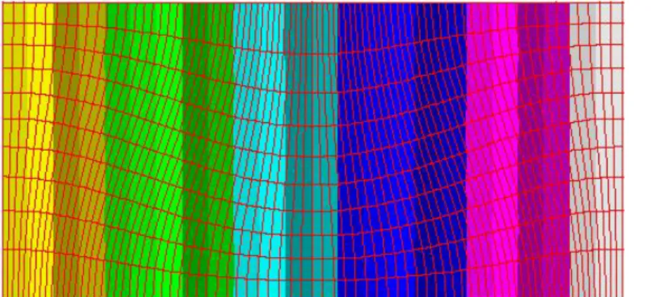
Grid distortion

3.1.3.1 The computational grid and accompanying depth profile. Bottom height ranging from -4 m (left) to -4.5 m (right)

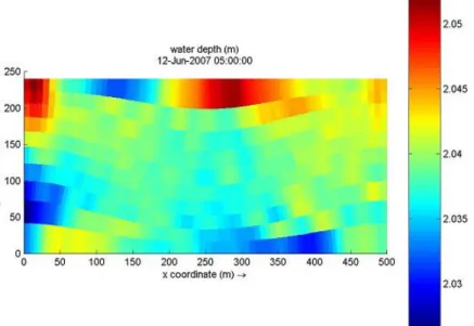
3.1.3.2 Water depth at the end of the simulation time (steady state solution)

3.1.3.3 Water depth at the end of the simulation time (steady state solution) with the extended grid

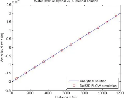
Wind driven channel flow

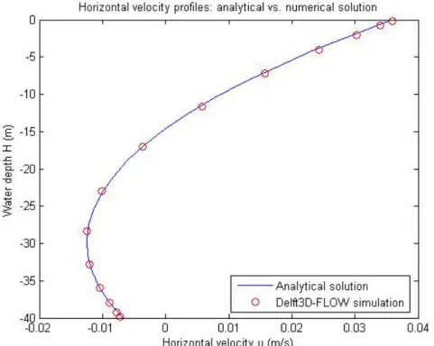
3.1.4.1 Water level for 5 m/s wind velocity (both analytical and numerical solutions) 3.1.4.2 Horizontal velocity profile for 5 m/s wind velocity (both analytical and numerical

(10)

3.1.4.3 Water level for 10 m/s wind velocity (both analytical and numerical solutions) 3.1.4.4 Horizontal velocity profile for 10 m/s wind velocity (both analytical and numerical

solutions).

Lock exchange flow

3.1.5.1 Initial distribution of salinity

3.1.5.2 Distribution of salinity at t = 120 s; hydrostatic mode 3.1.5.3 Distribution of salinity at t = 120 s; non-hydrostatic mode

Wave force and a mass flux in a closed basin

3.1.6.1 Wave force and mass flux effect

3.1.6.2 Water level (in m) along the basin; computed (in red) and according to the analytical solution (in black); on x-axis the x-coordinate (in m) of the basin

Flow over a weir

3.1.7.1 Cross sectional discharges for Cyclic scheme and a 30 m grid size 3.1.7.2 Cross sectional discharges for Flooding scheme and a 30 m grid size 3.1.7.3 Cross sectional discharges for Cyclic scheme and a 10 m grid size 3.1.7.4 Cross sectional discharges for Flooding scheme and a 10 m grid size

Coriolis testcase

3.1.8.1 The spherical-curvilinear 50x50 grid

3.1.8.2 Water level for the -plane solution. The analytical (initial) solution is depicted on the left and the numerical solution on the right

3.1.8.3 V-velocity for the -plane solution. The analytical (initial) solution is depicted on the left and the numerical solution on the

3.1.8.4 U-velocity for the -plane solution. The analytical (initial) solution is depicted on the left and the numerical solution on the right

Equilibrium slope for a straight flume

3.1.9.1 Equilibrium bed slope

Tidal flume

3.2.1.1 Computed and observed salt intrusion; -model 3.2.1.2 Computed and observed salt intrusion; Z-model

Water elevation in a wave flume

3.2.2.1 Bathymetry of laboratory experiment of Beji and Battjes

3.2.2.2 Water level history at a station located at 13.5 m from the inflow boundary Measurements in blue (with markers), Delft3D-FLOW results in red (no markers)

(11)

Vertical mixing layer (horizontal splitter plate)

3.2.3.1 Horizontal velocity profiles at 2 m, 5 m, 10 m and 40 m behind the splitter plate. Red circles represent the measurements and the solid lines represent the computed results

3.2.3.2 Density profiles at 2 m, 5 m, 10 m and 40 m behind the splitter plate. Red circles represent the measurements and the solid lines represent the computed results 3.2.3.3 Turbulent kinetic energy profiles at 2 m, 5 m, 10 m and 40 m behind the splitter

plate. Red circles represent the measurements and the solid lines represent the computed results

One-dimensional dam break

3.2.4.1 Water surface slope for a dam break scenario with initially dry bed

3.2.4.2 Water level for flooding of a dry bed, computed (in blue and black) and analytical (in red)

3.2.4.3 Water level for flooding of a wet bed, computed (in blue and black) and analytical (in red)

Horizontal mixing layer (vertical splitter plate)

3.2.5.1 Set-up of experiment (top view)

3.2.5.2 Computational grid at the tip of the splitter plate

3.2.5.3 Mixing layer thickness as a function of distance from the tip of the splitter plate (which lies at x = 0)

3.2.5.4 Observed (triangles) and simulated (lines) properties of mean flow and turbulence at a series of downstream cross sections; blue: offline computed flow

characteristics, red: online computed flow characteristics

Numerical scale model of an estuary

3.2.6.1 Detailed numerical scale model grid, Deurgangdock section, situation without dock 3.2.6.2 Depth of detailed numerical scale model, Deurgangdock section, situation without

dock

3.2.6.3 Computed (red) and measured (black) water levels at six stations along the flume on15 April 2003

3.2.6.4 Computed (red & magenta) and measured (blue & green) salinity at 7.2 cm - TAW in six stations along the flume on 15 April 2003

3.2.6.5 Computed (red) and measured (black) current magnitude and direction in four stations along the flume on 15 April 2003

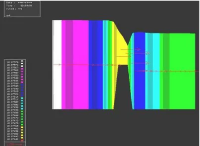
Numerical scale model of an estuary and a tidal dock

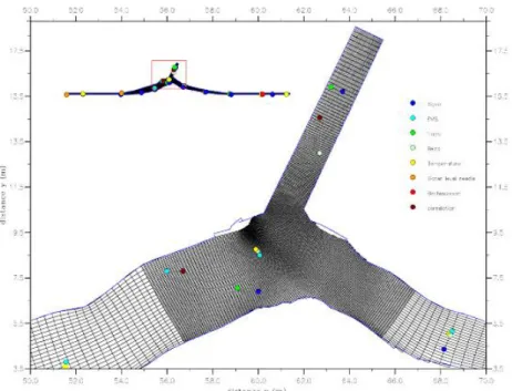
3.2.7.1 Numerical scale model grid for domain decomposition, situation with Deurgangdock and positions of instruments

(12)

3.2.7.2 Depth of numerical scale model with domain decomposition, situation with Deurgangdock

3.2.7.3 Computed (red) and measured (black) water levels at six stations along the flume on 26 May 2003

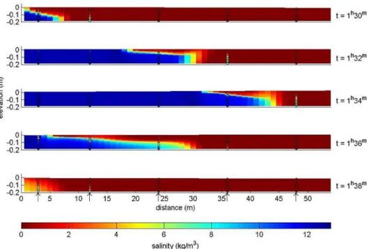
3.2.7.4 Computed (red & magenta) and measured (blue & green) salinity at six stations along the flume on 26 May 2003

3.2.7.5 Computed (red & magenta) and measured (blue & green) salinity at two stations in the Deurgangdock on 26 May 2003

3.2.7.6 Computed (red) and measured (black) current magnitude and direction in four stations along the flume on 26 May 2003

Two-dimensional dam break

3.2.8.1 Set-up of experiment

3.3.8.2 Three-dimensional surface level plot at the end of the wet-bed simulation 3.2.8.3 Three-dimensional surface level plot at the end of the dry-bed simulation

Curved back channel

3.3.1.1 Three applied grids: curvilinear, rectangular and rectangular with cut-cells

3.3.1.2 Velocity profile in the channel bend on the curvilinear, rectangular and the cut-cells grid

Drying and flooding

3.3.2.1 Bathymetry of the test case for drying and flooding

3.3.2.2 Time history of water levels (in m) for -model at two locations; on x-axis the time in minutes

3.3.2.3 Time history of water levels (in m) for Z-model at two locations; on x-axis the time in minutes

Schematized lake Veere model

3.3.3.1 Bathymetry for the two-dimensional model for Lake Veere

3.3.3.2 Change of salinity profile at pit 1 during the numerical simulation with the Z-model (solid line) and the -model (dash-dotted line)

3.3.3.3 Horizontal velocity at pit 1 after 1/6 (left plot) and at the end of the numerical simulation with the Z- (solid line) and the -model (dash-dotted line) 3.3.3.4 Vertical velocity at pit 1 after 1/6 (left plot) and at the end of the numerical

simulation with the Z- (solid line) and the -model (dash-dotted line)

Buoyant jet

3.3.4.1 Illustration of trajectory of bouyant plume

3.3.4.2 Temperature of the jet after 30 minutes, 1.5 hours, 2.5 hours, 3.5 hours and 4.5 hours, for the hydrostatic simulation

3.3.4.3 Temperature of the jet after 30 minutes, 1.5 hours, 2.5 hours, 3.5 hours and 4.5 hours, for the non-hydrostatic simulation

(13)

Migrating trench in a 1D channel

3.3.5.1 Measured and computed velocity and sediment concentration at the beginning of the morphological changes (T = 7.5 hours)

3.3.5.2 Measured and computed trench after 15 hours; initial trench (in green), computed trench after 15 hours (in black) and measured trench after 15 hours (in red)

Wind over a schematized lake

3.3.6.1 Bathymetry of schematized lake (depth in m) 3.3.6.2 Velocity field at steady state

North Sea

3.4.1.1 North Sea Survey cruise track (NSP project)

3.4.1.2 Computed surface and bottom temperatures for the period of 24 June to 19 July 1989

3.4.1.3 Observed surface and bottom temperatures for the period of 24 June to 19 July 1989 3.4.1.4 Computed surface and bottom temperatures for the period of 24 July to

9 August 1989

3.4.1.5 Observed surface and bottom temperatures for the period of 24 July to 9 August 1989

3.4.1.6 Computed surface and bottom temperatures for the period of 23 August to 2 September 1989.

3.4.1.7 Observed surface and bottom temperatures for the period of 23 August to 2 September 1989

3.4.1.8 Computed surface and bottom temperatures for the period of 7 September to 2 October 1989

3.4.1.9 Observed surface and bottom temperatures for the period of 7 September to 2 October 1989

3.4.1.10 Computed surface and bottom temperatures for the period of 7 October to 1 November 1989

3.4.1.11 Observed surface and bottom temperatures for the period of 7 October to 1 November 1989

3.4.1.12 Evolution thermal stratification at station A 3.4.1.13 Evolution thermal stratification at station B 3.4.1.14 Evolution thermal stratification at station C 3.4.1.15 Evolution thermal stratification at station D

(14)

Zegerplas

3.4.2.1 Schematic picture of the Zegerplas (left) and grid that was used (right) 3.4.2.2 Zegerplas, temperature distribution over layers of the -model for numerical

simulation of one year

3.4.2.3 Zegerplas, temperature distribution over layers of the Z-model for numerical simulation of one year

3.4.2.4 Zegerplas, temperature profile at RO371 (measured at August 14 1998 (the "+"-signs), measured at August 11 1999 (the crosses), and computed for

August 12 1996 (solid line)

Lake Grevelingen

3.4.3.1 Overview of the Lake Grevelingen measurement locations (red dots); cross-sections will be plotted along the red, dashed line

3.4.3.2 Time series of salinity (blue line) at 1 m (upper plot) and 15 m depth (lower plot) compared to measurements (red dots) at Station GTSO-08

3.4.3.3 Time series of temperature (blue line) at 1 m (upper plot) and 15 m depth (lower plot) compared to measurements (red dots) at Station GTSO-08

3.4.3.4 Z,t-diagrams of salinity (upper plot) and temperature (lower plot) for Station GTSO-08. The coloured dots represent measured values

3.4.3.5 Salinity contour plots at 1 m (upper plot) and 15 m depth (lower plot) compared to measurements (coloured dots) at 14 June

3.4.3.6 Temperature contour plots at 1 m (upper plot) and 15 m depth (lower plot) compared to measurements (coloured dots) at 14 June

3.4.3.7 Salinity (upper plot) and temperature (lower plot) along a cross section through Lake Grevelingen. The coloured dots represent measurements

Sea of Marmara

3.4.4.1 Computed (dashed line) and measured (solid line) water level elevation in Pendik (near southern Bosporus entrance) for December 2003

3.4.4.2 Computed (dashed line) and measured (solid line) water level elevation in Kavak (near northern Bosporus entrance) for January 2003

3.4.4.3 Modelled upper (blue), lower (red) and net (black) flux variation through northern cross section in the Bosporus for January 2003. The coloured dots represent fluxes derived from ADCP measurements (units are in km3/yr)

3.4.4.4 Modelled upper (blue), lower (red) and net (black) flux variation through northern cross section in the Bosporus for July 2003. The coloured dots represent fluxes derived from ADCP measurements (units are in km3/yr)

3.4.4.5 Time series of temperature (blue line) at 1 m (upper plot) and 40 m depth (lower plot) compared to measurements (red dots) at Station M23 in the north east of the Sea of Marmara

3.4.4.6 Z,t-diagrams of salinity (upper plot) and temperature (lower plot) for Station M23 in the north east of the Sea of Marmara. The coloured dots represent measured values

3.4.4.7 Z,t-diagrams of salinity (upper plot) and temperature (lower plot) for Station K2 in the south west of the Black Sea. The coloured dots represent measured values

(15)

3.4.4.8 Salinity (upper plot) and temperature (lower plot) along a cross section through the Dardanelles, the Sea of Marmara, the Bosporus and the south east of the Black Sea for January 21, 2003. The coloured dots represent measurements

3.4.4.9 Salinity (upper plot) and temperature (lower plot) along a cross section through the Dardanelles, the Sea of Marmara, the Bosporus and the south east of the Black Sea for July 5, 2003. The coloured dots represent measurements

3.4.4.10 Salinity (upper plot) and temperature (lower plot) along a cross section through the Bosporus for January 21, 2003. The coloured dots represent measurements

South China Sea

3.5.1.1 Surface layer temperature during the Northeast (NE, January) and Southwest (SW, August) monsoon highs. Model results compared with monthly-mean,

climatological Remotely Sensed Sea Surface Temperature (RS SST) data obtained from (Vazquez 2004)

3.5.1.2 Profile data at selected model stations. Model results (lower panel) compared with monthly-mean, climatological profile data from the World Ocean Atlas 2001 (upper panel) (Levitus 1982)

List of Abbreviations

2D Two dimensional

3D Three dimensional BSS Brier Skill Score

IAHR International Association of Hydraulics Engineering and Research SWE Shallow Water Equations

(16)

Summary

This document is the validation document for the mathematical model Delft3D-FLOW. The document is organised conforming to the Guidelines for documenting the validity of computational modelling software (IAHR, 1994).

The subject of this document is the validation of a computational model. The term computational model refers to software which primary function is to model a certain class of physical systems, and may include pre- and post-processing components and other necessary ancillary programmes. Validation applies primarily to the theoretical foundation and to the computational techniques that form the basis for the numerical and graphical results produced by the software. In the context of this document, validation of the model is viewed as the formulation and substantiation of explicit claims about applicability and accuracy of the computational results. This preface explains the approach that has been adopted in organising and presenting the information contained in this document.

Standard validation documents

This document conforms to a standard system for validation documentation. This system, the Standard Validation Document, has been developed by the hydraulic research industry in order to address the need for useful and explicit information about the validity of computational models. Such information is summarised in a validation document, which accompanies the technical reference documentation associated with a computational model. In conforming to the Standard, this validation document meets the following requirements:

1. It has a prescribed table of contents, based on a framework that allows separate quality issues to be clearly distinguished and described.

2. It includes a comprehensive list of the assumptions and approximations that were made during the design and implementation of the model.

3. It contains claims about the performance of the model, together with statements that point to the available substantiating evidence for these claims.

4. Claims about the model made in this document are substantiable and bounded: they can be tested, justified, or supported by means of physical or computational experiments, theoretical analysis, or case studies.

5. Claims are substantiated by evidence contained within this document, or by specific reference to accessible publications.

6. Results of validation studies included or referred to in this document are reproducible. Consequently the contents of this document are consistent with the current version of the software.

7. This document will be updated as the process of validating the model progresses.

Organisation of this document

Chapter 1 contains a short overview of the computational model and introduces the main issues to be addressed by the validation process. The model overview includes information about the purpose of the model, about pre- and post-processing options and other software

(17)

features, and about reference versions of the software. Validation priorities and approaches are briefly described, and a list of related documents is included.

Chapter 2 summarises the available information about the validity of the computational core of the model. In this chapter, claims are made about the range of applicability of the model and about the accuracy of computational results. Each claim is followed by a brief statement regarding its substantiation. This statement indicates the extent to which the claim has in fact been substantiated and points to the available evidence.

Chapter 3 contains such evidence, in the form of brief descriptions of relevant validation studies. Each description includes information about the purpose and approach of the study and a summary of main results and implications.

A glossary and complete list of references are contained in this document too.

A word of caution

This document contains information about the quality of a complex modelling tool. Its purpose is to assist the user in assessing the reliability and accuracy of computational results, and to provide guidelines with respect to the applicability and proper use of the modelling tool. This document does not, however, provide mathematical proof of the correctness of results for a specific application. The reader is referred to the License Agreement for pertinent legal terms and conditions associated with the use of the software.

The contents of this validation document attest to the fact that computational modelling of complex physical systems requires great care and inherently involves a number of uncertain factors. In order to obtain useful and accurate results for a particular application, the use of high-quality modelling tools is necessary but not sufficient. Ultimately, the quality of the computational results that can be achieved will depend upon the adequacy of available data as well as a suitable choice of model and modelling parameters.

Electronic standard validation document

This document is also available in electronic form in Portable Document Format (PDF). The electronic version may be read using the ACROBAT READERTM software which is available for many computer platforms.

The present version of the Validation Document Delft3D-FLOW (Version 1.0, 30 December 2007) can be downloaded from the Delft3D website:

http://www.wldelft.nl/soft/d3d/intro/validation/valdoc_flow.pdf

Acknowledgements

The guidelines [IAHR, 1994] provide a logical set up of the document. In the preparation of the present document, we aimed to share the look and feel with other validation documents in the market place, notably that of TELEMAC-2D [EDF-DRD, 2000] and of UnTRIM [Bundesanstalt für Wasserbau, 2002].

(18)

List of Symbols

Symbol Units Meaning

k

B

m2/s3 buoyancy flux term in transport equation for turbulent kinetic

energy

e

B

m2/s4 buoyancy flux term in transport equation for the dissipation of kinetic energy 2

,

D

C C

m1/2/s 2D Chézy coefficient 3D

C

m1/2/s 3D Chézy coefficient d

C

- wind drag coefficient

c

kg/m3 mass concentration

( )

c

kg/m3 mass concentration of sediment fraction

D

c

- constant relating mixing length, turbulent kinetic energy and

dissipation in the k model

p

c J/kg°C specific heat of sea water

c - calibration constant

'

c

- constant in Kolmogorov-Prandtl's eddy viscosity formulation

D kg/m2s deposition rate cohesive sediment

back

D

m2/s background turbulent eddy viscosity in x- and y-direction

,

h v

D D

m2/s eddy diffusivity in the horizontal and vertical direction

mol

D

m2/s molecular eddy diffusivity in x- and y-direction

d m water depth below some horizontal plane of reference (datum)

s

d

m representative diameter of suspended sediment 50

d

m median diameter of sediment

90

d

m sediment diameter

E m/s evaporation

E kg/m2s erosion rate cohesive sediment

x

F

m/s2 radiation stress gradient in x-direction

y

F m/s2 radiation stress gradient in y-direction

f

1/s Coriolis coefficient (inertial frequency) g m/s2 acceleration due to gravity

H m total water depth (

H

d

)

rms

H

m root-mean-square wave height

I m/s spiral motion intensity (secondary flow) k m2/s2 turbulent kinetic energy

s

k

m Nikuradse roughness length

L m mixing length

- index number of sediment fraction

S x

M kg m/s depth-averaged mass flux due to Stokes drift in x-direction S

y

(19)

M M m/s2 source or sink of momentum in x- and y-direction

n

m1/3/s Manning's coefficient P kg/ms2 hydrostatic water pressure

P m/s precipitation

k

P

m2/s3 production term in transport equation for turbulent kinetic energy P P kg/m2s2 gradient hydrostatic pressure in x- and y-direction

P

m2/s4 production term in transport equation for the dissipation of turbulent

kinetic energy

Q

m/s global source or sink per unit area

in

q

1/s local source per unit volume

out

q

1/s local sink per unit volume

R m radius of the Earth

Ri - gradient Richardson's number

S ppt salinity

b

S

- magnitude of the bed-load transport vector

s

_{relative density of sediment fraction. (} ₎

s w

T °C temperature (general reference)

T

°K temperature (general reference)

, ,

T T T kg/ms2 contributions secondary flow to shear stress tensor

t

s time

U m/s depth-averaged velocity in x-direction

ˆ

U

m/s velocity of water discharged in y-direction

u

m/s flow velocity in the x-direction

*

u

m/s friction velocity due to currents or due to current and waves *b

u

m/s friction velocity at the bed *

s

u m/s friction velocity at the free surface

U

m/s magnitude of depth-averaged horizontal velocity vector (U,V)T

10

U

m/s averaged wind speed at 10 m above free surface

ˆ

U

m/s velocity of water discharged in x- or y-direction

ˆ

_orb

U

m/s amplitude of the near-bottom wave orbital velocity

S

u

m/s Stokes drift in x- or y-direction

u m/s total velocity due to flow and Stokes drift in x- or y-direction

v

m/s fluid velocity in the y- direction

b

v

m/s velocity at bed boundary layer in y- direction V m/s depth-averaged velocity in y- direction

ˆ

V

m/s velocity of water discharged in y- direction

S

v

m/s Stokes drift in y- direction

v m/s total velocity due to flow and Stokes drift in x- direction

w

m/s fluid velocity in

z

-direction , 0

s

w m/s particle settling velocity in clear water (non-hindered) ( )

s

(20)

, ,

x y z

,

m Cartesian co-ordinates

0

z

m bed roughness length

c - coefficient to account for secondary flow in momentum equations

deg astronomical argument of a tidal component

t s computational time-step

( , )n m

x

m cell width in the

x

- direction, held at the V point of cell (n, m) ( , )n m

y

m cell width in the y- direction, held at the U point of cell (n, m)

b

z

m thickness of the bed layer

s

z

m thickness of the surface layer

b - thickness of the bed boundary layer in relative co-ordinates

m2/s4 dissipation in transport equation for dissipation of turbulent kinetic energy

m2/s3 dissipation in transport equation for turbulent kinetic energy emissivity coefficient of water at air-water interface

f m

2

/s fluid diffusion in the

z

- direction

f,x

,

f,y

,

f,z m

2

/s fluid diffusion coefficients in the x y z, , - directions, respectively

s m

2

/s sediment diffusion in the

z

- direction

s,x

,

s,y

,

s,z m

2

/s sediment diffusion coefficients in the x y z, , - directions, respectively

deg. latitude co-ordinate in spherical co-ordinates

J/sm2°C exchange coefficient for the heat flux in excess temperature model m equilibrium tide

e _m _{perturbation of the equilibrium tide due to earth tide} eo _m _{perturbation of the equilibrium tide due to tidal load}

o _m _{perturbation of the equilibrium tide due to oceanic tidal load}

deg longitude co-ordinate in spherical co-ordinates

d 1/s first-order decay coefficient

m2/s kinematic viscosity coefficient

back m

2

/s background turbulent eddy viscosity

H m

2

/s horizontal eddy viscosity in horizontal direction)

mol m

2

/s molecular eddy viscosity in horizontal direction)

V m

2

/s vertical eddy viscosity

2D m

2

/s part of eddy viscosity due to horizontal turbulence

3D m

2

/s part of eddy viscosity due to 3D turbulence kg/m3 density of water a kg/m 3 density of air 0 kg/m 3

reference density of water ( )

s kg/m

3

specific density of sediment fraction J/m2s°K4 Stefan-Boltsmann’s constant

(21)

-scaled vertical co-ordinate;

z

d

; (surface

0;

1

)

C - Prandtl-Schmidt number

kg/ms2 shear stress

b N/m

2

bed shear stress due to current and waves

b kg/ms

2

bed shear stress in x-direction

b kg/ms

2

bed shear stress in y-direction

c kg/ms

2

magnitude of the bed shear stress due to current alone

w kg/ms

2

magnitude of the at bed shear stress due to waves alone

m kg/ms

2

magnitude of the wave-averaged at bed shear stress for combined waves and current

,

b c kg/ms

2

bed shear stress due to current

,

b cr kg/ms

2

critical bed shear stress

,

b cw kg/ms

2

bed shear stress due to current in the presence of waves

,

b w kg/ms

2

bed shear stress due to waves

cr kg/ms

2

critical bed shear stress

,

cr d kg/ms

2

user specified critical deposition shear stress

,

cr e kg/ms

2

user specified critical erosion shear stress

cw kg/ms

2

mean bed shear stress due to current and waves

max kg/ms

2

maximum bottom shear stress with wave-current interaction

mean kg/ms

2

mean (cycle averaged) bottom shear stress with wave-current interaction

s kg/ms

2

shear stress at surface in x-direction

s kg/ms

2

shear stress at surface in y-direction

m/s velocity in the -direction in the - co-ordinate system 1/s angular frequency waves

deg./hour angular frequency of tide and/or Fourier components

,

horizontal, curvilinear co-ordinates

J/m2s heat flux through free surface

m water level above some horizontal plane of reference (datum)

b _m _{bottom tide}

e _m _{earth tide}

(22)

(23)

1 Introduction

This chapter refers to the model Delft3D-FLOW as a software product, and clarifies the relation of that which is being validated to the rest of the software. It includes brief descriptions of pre- and post-processing options, as well as an explanation of the modular structure of the computational core of the model.

Delft3D-FLOW is the hydrodynamic module of Delft3D, which is Delft Hydraulics' fully-integrated program for the modelling of water flows, waves, water quality, particle tracking, ecology, sediment and chemical transports and morphology. In Figure 1.1 a system overview of Delft3D is given.

Figure 1.1: System overview of Delft3D

We note that in previous versions of Delft3D also contained a MOR(phology) module. However, the morphology functionality is now part of the FLOW module and a separate MOR module does not exist anymore.

The present Validation Document concerns the properties and validity of Delft3D-FLOW. It focuses on the computational part of Delft3D-FLOW. For example, the pre- and postprocessing, and the coupling with other modules in Delft3D, such as WAVE, WAQ, PART and ECO, are beyond the scope of this description.

1.1 Model overview

1.1.1 Purpose

The primary purpose of the computational model Delft3D-FLOW is to solve various one-, two- and three-dimensional, time-dependent, non-linear differential equations related to hydrostatic and non-hydrostatic free-surface flow problems on a structured orthogonal grid to cover problems with complicated geometry. The equations are formulated in orthogonal curvilinear co-ordinates on a plane or in spherical co-ordinates on the globe. In Delft3D-FLOW models with a rectangular or spherical grid (Cartesian frame of reference) are considered as a special form of a curvilinear grid, see [Kernkamp et al., 2005] and [Willemse et al., 1986].

(24)

The equations solved are mathematical descriptions of physical conservation laws for:

water volume (continuity equation),

linear momentum (Reynolds-averaged Navier-Stokes (RANS) equations), and tracer mass (transport equation) , e. g. for salt, heat (temperature) and suspended sediments or passive pollutants.

Furthermore, bed level changes are computed, which depend on the quantity of bottom sediments.

The following physical quantities can be obtained in dependence on three-dimensional space(x,y,z)and timet:

water surface elevation (x,y,t) with regard to a reference surface (e. g. mean sea level), current velocityu(x,y,z,t), v(x,y,z,t), w(x,y,z,t),

non-hydrostatic pressure componentq(x,y,z,t),

tracer concentration C(x,y,z,t), e. g. temperature, salinity, concentration of suspended sediments or passive pollutants; and

bed leveld(x,y,t),representing changes in bathymetry.

Delft3D-FLOW can be used in either hydrostatic or non-hydrostatic mode. In case of hydrostatic modelling the so-called shallow water equations are solved, whereas in hydrostatic mode the Navier-Stokes equations are taken into account by adding non-hydrostatic terms to the shallow water equations. A fine horizontal grid is needed to resolve non-hydostatic flow phenomena.

When the computational model Delft3D-FLOW is used in one- or two-dimensional mode (with onez-layer in vertical direction) the results foru, v andCwill be the respective depth averaged values for current velocity and tracer concentration.

For the vertical grid system two options are available in Delft3D-FLOW, namely so-called - or z-coordinates. For a detailed discussion of these two grid systems we refer to Section 1.1.4. In the remainder of this document “z” will be used as vertical coordinate.

1.1.2 Properties of the computational model

The computational model Delft3D-FLOW can be characterised by means of the following distinguished properties:

Grid alignment with complicated boundaries and local grid refinements to meet the needs of resolving finer spatial resolution in various numerical modelling tasks, which results in an accurate description of geometry (orthogonal curvilinear grid, see Figure 1.2);

application for one- and two-dimensional vertically averaged as well as hydrostatic or non-hydrostatic three-dimensional problems;

a solution technique that allows for solution based on accuracy considerations rather than stability (alternating direction implicit finite difference method);

(25)

conservation of fluid and tracer mass locally and globally; computationally efficient and robust;

a computational core and a separate user interface.

efficient coupling with other physical processes via the other modules of the integrated Delft3D modelling system.

1.1.3 Horizontal grid

In Delft3D-FLOW the horizontal physical model domain(x,y) is covered with a curvilinear orthogonal grid, designed and optimised for a given application through a grid generator. This includes simple rectangular, spherical and curvilinear grids. The computations are performed on a transformed, simple rectangular computational domain. For the horizontal direction the grid concept is illustrated in Figure 1.2.

+ + + + + + + + + + + + + + + + + + + + + + + + + + + + + + + + + + + + + + + + + + + + + + + + + + + + + + + + + + + + + + + + + + + + + ++ + + + + + + ++ ++ C e l l d r a w n b y p l o t p r o g r a m s , R G F G R I D a n d Q U I C K I N + W a t e r l e v e l p o i n t i M o d e l b o u n d a r i e s I d e n t i c a l g r i d i n d e x n u m b e r P o i n t s re q u i r e d b y I f o r b o u n d a r y d e f i n i t i o n / s p e c . ++ + + + + + + o o o o o o o o o o o o o o o o o o o o o o o o o o o o o o o o o o o o o o o o o o o o o o o _o o _o o o o o o o o o o o o o o o o D e p t h p o i n t i

Figure 1.2 Horizontal curvilinear grid concept

1.1.4 Vertical grid

3D numerical modelling of the hydrodynamics and water quality in these areas requires accurate treatment of the vertical exchange processes. The existence of vertical stratification influences the turbulent exchange of momentum, heat, salinity and passive contaminants. The accuracy of the discretisation of the vertical exchange processes is determined by the vertical grid system. The vertical grid should:

(26)

resolve the boundary layer near the bottom and surface to allow an accurate evaluation of the bed stress and surface stresses, respectively;

be fine around pycnoclines;

avoid large truncation errors in the approximation of strictly horizontal gradients.

The two commonly used vertical grid systems in 3D shallow-water models are the z-coordinate system (Z-model) and the so-called -coordinate system ( -model), see Figure 1.3. Neither meets all the requirements. The Z-model has horizontal coordinate lines which are (nearly) parallel with isopycnals, but the bottom is usually not a coordinate line and is represented instead as a staircase (zig-zag boundary). This leads to inaccuracies in the approximation of the bed stress and the horizontal advection near the bed. The sigma-model has quasi-horizontal coordinate lines. The first and last grid line follow the free surface ( = 0) and the sea bed boundary ( = -1), respectively, with a user defined -distribution in between. The grid lines follow the bottom topography and the surface but generally not the isopycnals. Inaccuracies associated with these numerical artefacts have been addressed in Delft3D, which has led to acceptable solutions for practical applications.

In Delft3D-FLOW both the options of fixed horizontal layers (Z-model) and the sigma grid ( -model) are operational. The two grid concepts are illustrated in Figure 1.3.

In practice, this means that depending on the application the user can choose the best option for the representation of the processes in the vertical. In case of stratified flow problems in coastal seas, estuaries and lakes where steep topography is a dominant feature, this is an important issue. For lakes a Z-model is preferred, because the vertical exchange process should not be dominated by truncation errors.

1.1.5 Pre- and post-processing and other software features

Delft3D-FLOW can be used as a stand-alone software package. For using Delft3D-FLOW the following auxiliary software tools are important:

(27)

RGFGRID for generating and optimising curvilinear grids QUICKIN for preparing and manipulating grid oriented data,

such as bathymetry or initial conditions for water levels, salinity or concentrations of constituents. Delft3D-FLOW GUI Graphical user Interface for preparing a complete

Delft3D-FLOW input file, which is called a Master Definition (MD) file.

TRIANA for performing off-line tidal analysis of time series generated by Delft3D-FLOW

TIDE for performing tidal analysis on time-series of measured water levels or velocities

NESTHD for generating (offline) boundary conditions from an overall model for a nested model

GPP for visualisation and animation of simulation results QUICKPLOT for visualisation and animation of simulation

results; package based on MATLAB

Table 1.1 Overview of auxiliary software tools for Delft3D-FLOW

For details on using these utility programs we refer to the respective User Manuals.

1.1.6 Version information

The content of this document is consistent with the (operational) version 3.55.04 of the Delft3D-FLOW software, which has been released in November 2007 [WL | Delft Hydraulics, 2007].

1.2 Validation priorities and approaches

In this DELFT3D-FLOW validation document at first the model functionality of Delft3D-FLOW is described by means of its applications (see Chapter 2.2.1) and its physical processes (see Chapter 2.2.2). Next, the following three phases are distinguished:

Conceptual model (mathematical description of a physical system together with some fundamental assumptions and/or simplifications), see Chapter 2.3.

Algorithmic implementation (conversion of the conceptual model into a set of procedures for computation; e.g., discretisations, solution procedures), see Chapter 2.4.

Software implementation (conversion of algorithmic implementation into computer code; coding of algorithms, data structures, etc.), see Chapter 2.5.

These three phases are according to the IAHR guidelines for validation, as described in [IAHR, 1994], see also [Dee, 1993].

In Chapter 3 the claims and substantiations that have been formulated in Chapter 2 for the model functionality, the conceptual model, the algorithmic implementation and the software implementation of Delft3D-FLOW are validated for a large number of validation studies.

(28)

This Delft3D-FLOW validation document, the input and result files of the validation studies (of Chapter 3) can be supplied to users of the Delft3D-FLOW system, so that they are able to verify the validity and performance of Delft3D-FLOW.

1.3 Quantification of model output

This version hardly contains any quantification of model results. All validation studies have been described and lot of figures are shown. By visual inspection and by reading the conclusions for each validation study, the reader will have an impression of the quality of the computed results. However, a quantitative assessment of the accuracy of model predictions is lacking. In a next version of this validation document, a quantitative assessment will be added.

For a quantitative assessment various options are available. Preferably, a uniform performance indicator will be applied for all validation studies, possibly supported by additional quantification parameters. An appropriate candidate might be the so-called Brier Skill Score (BSS), which is an objective performance indicator. TheBSS is defined as:

2 2

Y

X

BSS =1

B

X

(1.3.1)

where Y is the set of predictions, X is the set of measurements/analytical data and B is a baseline prediction. The difficulty lies in choosing a suitable baseline prediction. TheBSS can be derived for each test case, for one or more key parameters. TheBSS is independent of the type of model, i.e. tidal forcing, transport [Murphy et al., 1989]. For more details, we refer to [Wallingford, 200X].

1.4

1.5 Project team

This validation document has been prepared by Herman Gerritsen and Erik de Goede. The figures and WL | Delft Hydraulics Wiki/Internet pages with model results of the validation studies have been prepared by Frank Platzek, Menno Genseberger. Rob Uittenbogaard, Firmijn Zijl, Daniel Twigt and Jan van Kester have provided valuable assistance.

(29)

1.6 Status of current version

The present version of the Validation Document Delft3D-FLOW (Version 1.0, 30 December 2007) is a complete version. The previous version (Version 0.3, dated 16 March 2004) contained results for only two validation studies, namely the tidal flume and the North Sea validation studies. This version is complete with respect to the description of the model validity, the conceptual model, the algorithmic implementation, the software implementation and the validation for all validation studies.

However, twenty-nine validation studies are reported in this validation document. It is evident that all functionality in Delft3D-FLOW can not be validated with twenty-nine studies. For example, only a few morphologic studies are reported and the reader is referred to other documents such as [WL | Delft Hydraulics, 1994]. Nevertheless, this document provides a clear view of what is possible with Delft3D-FLOW.

Moreover, a quantitative assessment of the Delft3D-FLOW model accuracy is lacking and will be incorporated in a next version.

(30)

(31)

2 Model validity

This chapter summarises all available information pertaining to the validation of the computational core of the model. This includes the assumptions and approximations that were introduced during the design and implementation of the model. It further includes claims about the applicability and/or accuracy of (aspects of) the model, together with statements about the substantiations of those claims.

The nature of a claim and its substantiation varies depending on the subject, as explained below under the headings of the various subsections in which they appear. We have aimed to make claims as explicit as possible and to provide useful information about model validity. Substantiation aims to be thorough but brief, which can be achieved by using references.

Note that a substantiation may be incomplete, due to the nature of the claim, or because the evidence is not (yet) available. In such cases we prefer to admit this rather than to invent a substantiation that appears convincing.

These claims and substantiations together comprise the essential information in this document. The remainder of the document serves either to provide context, necessary background material or substantiating evidence.

2.1 Physical system

This section describes the physical system or systems being modelled. It describes what is being modelled, rather than how it is being modelled. The hydrodynamic module Delft3D-FLOW simulates two-dimensional (2D, depth-averaged) or three-dimensional (3D) unsteady flow and transport phenomena resulting from tidal and meteorological forcing, including the effect of density differences due to a non-uniform temperature and salinity distribution (density-driven flow). The flow model can be used to predict the flow in shallow seas, coastal areas, estuaries, lagoons, rivers and lakes. It aims to model flow phenomena of which the horizontal length and time scales are significantly larger than the vertical scales, which is the so-called shallow water assumption.

If the fluid is vertically homogeneous, a depth-averaged approach is appropriate. Delft3D-FLOW is able to run in two-dimensional mode (one computational layer), which corresponds to solving the depth-averaged equations. Examples in which the two-dimensional, depth-averaged flow equations can be applied are tidal waves, storm surges, tsunamis, harbour oscillations (seiches) and transport of pollutants in vertically well-mixed flow regimes.

Three-dimensional modelling is of particular interest in transport problems where the horizontal flow field shows significant variation in the vertical direction. This variation may be generated by wind forcing, bed stress, Coriolis force, bed topography or density differences. Examples are dispersion of passive materials or cooling water in lakes and coastal areas, upwelling and downwelling of nutrients, salt intrusion in estuaries, fresh water river discharges in bays and thermal stratification in lakes and seas.

(32)

2.2 Model functionality

This section describes the functionality of the model by referring to specific instances or configurations of the physical system described in Section 2.1 above. It consists of claims about what the model is actually able to represent, and (to the extent that this is possible) how well it does so. For the purposes of this section the model can be regarded as a black box, taking input information and producing computational results.

2.2.1 Applications

This section presents an overview of the domain of applicability of the model. This is done by making claims about the types of practical and realistic situations in which the model can be employed, and showing the nature and quality of the information that the model is capable of generating in those situations.

The purpose of providing the reader with this inventory of application types is to allow the reader to quickly recognise whether the model is indeed suitable for a particular application.

The computational model Delft3D-FLOW can be used in a wide range of applications, which are listed below:

Tide and wind-driven flow resulting from space and time varying wind and atmospheric pressure (See Section 2.2.1.1)

Density driven flow and salinity intrusion (See Section 2.2.1.2) Wind driven flow (See Section 2.2.1.3)

Horizontal transport of matter on large and small scales (See Section 2.2.1.4).

Hydrodynamic impact of engineering works such as land reclamation, breakwaters, dikes (See Section 2.2.1.5)

Hydrodynamic impact of hydraulic structures such as gates, weirs, barriers and floating structures (See Section 2.2.1.6)

Spreading of waste water discharges from coastal outfalls (See Section 2.2.1.7)

Thermal recirculation of cooling water discharges from a power plant (See Section 2.2.1.8)

Hydrostatic and non-hydrostatic flow (See Section 2.2.1.9).

Thermal stratification in seas, lakes and reservoirs (See Section 2.2.1.10). Small scale current patterns near harbour entrances (See Section 2.2.1.11). Flows resulting from dam breaks (See Section 2.2.1.12).

The model results have the form of distributions of the simulated quantities (water levels, currents, salinity, temperature, pollutant concentrations) in all grid points at user specified points in time, plus detailed time series of such parameters at user-selected locations. Each application is described in more detail in subsequent sections.

(33)

Tidal dynamics of estuaries or coastal seas

Claim 2.2.1.1: Delft3D-FLOW can be used for an accurate prediction of the tidal dynamics (water elevation, currents) in estuaries or coastal seas.

Substantiation: Validation Study 3.1.1 (Simple channel flow);

Validation Study 3.2.6 (Numerical scale model of an estuary).

Validation Study 3.2.7 (Numerical scale model of an estuary and a tidal lock).

Validation Study 3.4.1 (North Sea).

Example(s) of application studies:

1. 2D tidal modelling of the Indonesian waters using a spherical grid modelling approach, [Gerritsen et al., 2003]

2. 3D tidal modelling of the North Sea in the curvilinear PROMISE model, [Gerritsen et al., 2000]

Density driven flow and salinity intrusion

Claim 2.2.1.2: Delft3D-FLOW can be used for an accurate prediction of the density (salinity and/or temperature) driven flow. Moreover, sediment concentrations can be taken into account with respect to density values.

Substantiation: Validation Study 3.1.5 (Lock exchange flow);

Validation Study 3.2.6 (Numerical scale model of an estuary).

Validation Study 3.2.7 (Numerical scale model of an estuary and a tidal lock).

Validation Study 3.2.1 (Tidal flume).

1. Baroclinic adjustment of an initial density front [Tartinville et al., 1998] 2. Tidal flume [Karelse, 1996]

3. Salinity and temperature stratification in the Rhine plume [De Kok et al., 2001] 4. Salinity stratification in Hong Kong waters [Postma et al., 1999]

Wind driven flow and storm surges

Claim 2.2.1.3: Delft3D-FLOW can be used for an accurate prediction of wind driven flow and storm surges.

Substantiation: Validation Study 3.1.4 (Wind driven channel flow). Validation Study 3.4.1 (North Sea).

1. 2D tidal and surge modelling in the North Sea [Gerritsen et al., 1995; Gerritsen and Bijlsma, 1988]

2. Cyclone-induced storm surges in the Bay of Bengal [Vatvani et al., 2002] 3. North Sea storm surge model [Verboom et al., 1992]

(34)

Horizontal transport of matter on large and small scales

Claim 2.2.1.4: Delft3D-FLOW can be used for an accurate prediction of horizontal transport of matter, both on large and small scales.

Substantiation: Validation Study 3.1.5 (Lock exchange flow); Validation Study 3.2.1 (Tidal flume)

1. 3D sediment transport in the North Sea on seasonal scales [Gerritsen et al., 2000] 2. Midfield spreading of matter from an outfall [Gerritsen and Verboom, 1994]

Hydrodynamic impact of engineering works

Claim 2.2.1.5: Delft3D-FLOW can be used to investigate the hydrodynamic impact of engineering works, such as land reclamation, breakwaters and dikes.

Substantiation: Not in list of validation studies yet.

1. Impacts of Maasvlakte 2 on the Wadden Sea and North Sea coastal zone [De Goede et al., 2005]

Hydrodynamic impact of hydraulic structures

Claim 2.2.1.6: Delft3D-FLOW can be used to investigate the hydrodynamic impact of hydraulic structures, such as gates, weirs and barriers.

Substantiation: Validation Study 3.1.7 (Flow over a weir).

1. Complex flows around groynes [Van Schijndel and Jagers, 2003] 2. Impact of coastal structures [Roelvink et al., 1999]

Spreading of waste water discharges from coastal outfalls

Claim 2.2.1.7: Delft3D-FLOW can be used for an accurate prediction of waste water dispersion from coastal outfalls.

(35)

Thermal recirculation of cooling water discharges

Claim 2.2.1.8: Delft3D-FLOW can be used to describe and quantify the thermal recirculation between discharge and intake points, by which e.g. the design and efficiency of a power plant can be assessed.

1. Thermal discharges for the Maasvlakte-2 [Kleissen, 2007]

2. Pembroke Power Station, marine discharge study-phase 2, 3D hydrodynamic and water quality model [Karelse and Hulsen, 1995]

Hydrostatic and non-hydrostatic flow

Claim 2.2.1.9: Delft3D-FLOW can be used for an accurate prediction of hydrostatic and non-hydrostatic flow. Depending on the application (ratio between horizontal and vertical length scale), the user can choose the most suitable modelling approach.

Substantiation: Validation Study 3.1.5 (Lock exchange flow); Validation Study 3.3.4 (Buoyant yet).

1. 2D and 3D transport in the North Sea on seasonal scales [Gerritsen et al., 2000] 2. Near-field and far-field modelling of bouyant discharges [Van der Kaaij, 2007]

Thermal stratification in seas, lakes and reservoirs

Claim 2.2.1.10: Delft3D-FLOW can be used for an accurate prediction of thermal stratification in seas, lakes and reservoirs

Substantiation: Validation Study 3.3.3 (Schematised Lake Veere); Validation Study 3.4.1 (North Sea);

Validation Study 3.4.2 (Zegerplas).

1. Seasonal temperature stratification in the North Sea [De Kok et al. 2001]

(36)

Small scale current patterns near harbour entrances

Claim 2.2.1.11: Delft3D-FLOW can be used for an accurate prediction of small scale current patterns near harbour entrances. For example, a so-called Horizontal Large Eddy Simulation (HLES) can be applied to resolve small scale turbulent behaviour.

Substantiation: Validation Study 3.2.5 (Horizontal mixing layer).

1. Stroomonderzoek Sluizen IJmuiden [Van Banning, 1995]

2. Numeriek modelonderzoek naar de reductie van de neer in de monding van de voorhaven van IJmuiden [Bijlsma, 2007]

Flows resulting from dam breaks

Claim 2.2.1.12: Delft3D-FLOW can be used for an accurate prediction of flows resulting from dam breaks.

Substantiation: Validation Study 3.2.4 (Two-dimensional dam break).

1. A numerical method for every Froude number in shallow water flows, including large scale inundations. [Stelling and Duinmeijer, 2003]

2.2.2 Processes

This section further characterises the domain of applicability of the model. This is done by making claims about the individual physical processes represented in Delft3D-FLOW. The idea is to break down the physics into elements that are as simple as possible, yet still meaningful.

The information contained in this section supplements that in the previous section. It is intended to allow the reader to judge whether or not the model is suitable for his purpose, by considering separately the individual processes that play a role in the application he has in mind.

Delft3D-FLOW is able to represent a large number of processes, which are listed below: Propagation of long waves (barotropic flow) (See Section 2.2.2.1)

Baroclinic flow, salinity, suspended sediment and temperature driven flow, including prognostic or diagnostic modelling (See Section 2.2.2.2)

Transport of dissolved material and pollutants (See Section 2.2.2.3)

Transport of sediments, including erosion, sedimentation and bed load transport (See Section 2.2.2.4)

Propagation of short waves (See Section 2.2.2.5) Subcritical and supercritical flow (See Section 2.2.2.6) Steady and unsteady (time varying) flow (See Section 2.2.2.7) Drying and flooding of intertidal flats (See Section 2.2.2.8)

(37)

Turbulent mixing (See Section 2.2.2.10)

Time varying sources and sinks; e.g. river discharges (See Section 2.2.2.11)

Impact of space and time varying wind shear stress at the water surface (See Section 2.2.2.12)

Impact of space varying shear stress at the bottom (See Section 2.2.2.13)

Impact of space and time varying atmospheric pressure on the water surface (See Section 2.2.2.14)

Heat exchange through the free surface, evaporation and precipitation (See Section 2.2.2.15)

Wave driven currents (See Section 2.2.2.16)

Impact of secondary flow on depth-averaged momentum equations (See Section 2.2.2.17)

Barotropic tide generation (See Section 2.2.2.18)

In subsequent sections each process will be described in more detail.

Propagation of long waves

Description: For long waves (in shallow water) the vertical acceleration can be assumed to be negligible and the pressure to be hydrostatic. Under these assumptions the celerity of the wave only depends on gravity and water depth. It is also independent of the wave length. Relevant examples of long waves are tidal waves. The free surface gradients represent so-called barotropic flow. A special surface gradients generated by of long waves are the surges along coasts generated by wind (storm surge modelling).

Claim 2.2.2.1: Delft3D-FLOW can accurately simulate the propagation of long waves.

Substantiation: Validation Study 3.1.2 (Standing wave);

1. Tidal propagation for the North Sea [Gerritsen and Verboom, 1994; Gerritsen and Bijlsma, 1988; Gerritsen et al., 1995)]

2. Irish Sea Model [Hulsen, 1989]

3. South China Sea Model [Gerritsen et al., 2000;Schrama, 2002, Twigt et al., 2007] 4. Tide in the Westerschelde estuary [Wang et .al., 2002]

(38)

Baroclinic flow - salinity and temperature driven flow

Description: Baroclinic flow is the result of varying density in horizontal direction, due to salinity and or temperature differences. The salinity and temperature can either be model variables in their own (fully baroclinic flow), or can be prescribed as fixed distributions (diagnostic flow).

Claim 2.2.2.2: Delft3D-FLOW can accurately simulate density driven (or baroclinic) flows.

Substantiation: Validation Study 3.1.5 (Lock exchange flow with hydrostatic pressure or non-hydrostatic pressure).

Validation Study 3.2.1 (Salt intrusion in laboratory flume)

Validation Study 3.2.6 (Salt intrusion in 3D Numerical Scale Model with -coordinates of an estuary)

Validation Study 3.2.7 (3D Numerical Scale Model with -coordinates and HLES for the complex exchange flow between a tidal dock and the estuary)

Validation Study 3.4.1 (3D -model of the North Sea) Validation Study 3.4.3 (3D Z-model of Lake Grevelingen) Validation Study 3.4.4 (3D Z-model of Sea of Marmara) Validation Study 3.4.5 (3D -model of the South China Sea)

Transport of dissolved material and pollutants

Description: In estuaries and coastal seas spreading of dissolved material and suspended sediment which moves with the flow.

Claim 2.2.2.3: Delft3D-FLOW can accurately simulate the (advective and diffusive) transport of dissolved material, suspended sediment and pollutants.

Substantiation: Validation Study 3.2.6 (Numerical scale model of an estuary).

Validation Study 3.2.7 (Numerical scale model of an estuary and a tidal dock).

(39)

Transport of sediments, including erosion, sedimentation and bed

load transport

Description: Transport of suspended sediment contributes to a large amount to the total sediment transport in estuaries and coastal seas. In the stratified and/or gradient zone of an estuary a turbidity maximum, formed by accumulation of suspended sediments, is a common phenomenon.

Claim 2.2.2.4: Delft3D-FLOW can accurately simulate the transport of sediment, both in horizontal and vertical direction including deposits (deposition) and uptake (erosion) at the water-bottom interface.

Substantiation: Validation Study 3.1.9 (Equilibrium slope for a straight channel). Validation Study 3.3.7 (migrating trench in a 1D channel)

1. Suspended sediment modelling in a shelf sea ([Gerritsen et al., 2000]

Reference: [WL | Delft Hydraulics, 1994]

Propagation of short waves

Description: For short waves the vertical acceleration of the fluid can no longer be neglected and the pressure is non-hydrostatic. The celerity of the wave then depends on gravity, water depth as well as wave length.

Claim 2.2.2.5: Delft3D-FLOW can accurately simulate the propagation of short waves.

Substantiation: Validation Study 3.1.5 (Lock exchange flow);

Validation Study 3.2.2 (Water elevation in a wave flume).

Subcritical and supercritical flow

Description: In shallow water flow different flow regimes occur, such as subcritical or supercritical flows. Supercritical flow e.g. occurs near hydraulic structures such as weirs and barriers or are generated by sills on the bottom, or during flooding of an initial dry bed (dam break problem).

Claim 2.2.2.6: Delft3D-FLOW can accurately simulate subcritical and supercritical flows and the transition region when the flow changes from subcritical to supercritical or vice versa. Such conditions may e.g. occur in case of hydraulic jumps.

Substantiation: Validation Study 3.2.4 (One-dimensional dam break); Validation Study 3.2.8 (Two-dimensional dam break).

(40)

Reference: A numerical method for every Froude number in shallow water flows, including large scale inundations. [Stelling and Duinmeijer, 2003]

Steady and unsteady flow

Description: The Delft3D-FLOW system has been developed for simulating unsteady shallow water flow. However, the system can also be used for simulating steady state systems. In particular, this is relevant for river applications, which often are modelled with steady boundary conditions as forcing. The boundary conditions determine the steady state solution, while the initial conditions determine the spinning up period of the model.

Claim 2.2.2.7: Delft3D-FLOW can accurately simulate steady and unsteady flow.

Substantiation: All validation studies are relevant to this claim.

Drying and flooding of intertidal flats

Description: In estuaries and coastal seas with significant tidal range quite often vast areas of land (tidal fiats) are subsequently covered and uncovered with water during each tidal cycle.

Claim 2.2.2.8: Delft3D-FLOW can accurately simulate drying and flooding of tidal areas.

Substantiation: Validation Study 3.2.4 (1D dam break).

Reference(s): [Vatvani et al., 2002], [Stelling and Duinmeijer, 2003].

The effect of the Earth's rotation (Coriolis force)

Description: Earth rotation results in inclination of flows to the right on the northern hemisphere, and to the left on the southern hemisphere. The Coriolis parameterf depends on the geographic latitude and the angular speed of rotation of the earth, :

f

2 sin

. This results in an inclination of the flow direction, which varies with the depth and also depends on the latitude.

Claim 2.2.2.9: Delft3D-FLOW can take into account the impact of the Coriolis force arising from the rotation of the earth.