FPGA–BASED EFFICIENT HARDWARE/SOFTWARE
CO–DESIGN FOR INDUSTRIAL SYSTEMS WITH
CONSIDERATION OF OUTPUT SELECTION
Kyriakos M. Deliparaschos
∗— Konstantinos Michail
∗∗Argyrios C. Zolotas
∗∗∗— Spyros G. Tzafestas
∗∗∗∗This work presents a field programmable gate array (FPGA)-based embedded software platform coupled with a software-based plant, forming a hardware-in-the-loop (HIL) that is used to validate a systematic sensor selection framework. The systematic sensor selection framework combines multi-objective optimization, linear-quadratic-Gaussian (LQG)-type control, and the nonlinear model of a maglev suspension. A robustness analysis of the closed-loop is followed (prior to implementation) supporting the appropriateness of the solution under parametric variation. The analysis also shows that quantization is robust under different controller gains. While the LQG controller is implemented on an FPGA, the physical process is realized in a high-level system modeling environment. FPGA technology enables rapid evaluation of the algorithms and test designs under realistic scenarios avoiding heavy time penalty associated with hardware description language (HDL) simulators. The HIL technique facilitates significant speed-up in the required execution time when compared to its software-based counterpart model.
K e y w o r d s: sensor optimization, FPGA, maglev, embedded control, electromagnetic suspension, linear quadratic Gaussian, hardware-in-the-loop, FPGA-in-the-loop
1 INTRODUCTION
Most control systems nowadays are embedded in a sense that they rely on built-in special purpose digital hardware to close any feedback loops. Embedded con-trol systems are widely used in industrial concon-trol, trans-portation systems, robotics, automobiles, aircrafts (incl. UAVs), household appliances and other. These types of system interface with the external environment (ie, sen-sors and actuators) are real-time critical (ie, embedded control algorithm must execute in synchrony with the physical system which is controlled to guarantee perfor-mance and safety), as well as allowing for distributed control (ie, a network of embedded controllers). A model-based embedded control software/hardware co-design ap-proach is followed in this work. Modeling/simulation alongside FPGA synthesis and HDL analysis tools (ie, MATLAB/Simulink and Xilinx ISE) is used to enable rapid prototyping, autocode generation (ie, generate HDL code from a Simulink model), Hardware-In-the-Loop (HIL) testing, and consider the functional correct-ness of the model-based design with the generated HDL in a co-simulation environment. HIL techniques are widely used in the development and testing of complex real-time control systems by effectively adding the complexity of the plant under control to the test platform [1, 2]. The model of the system is realized in soft form and modeled
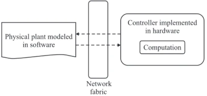
via high-level language (eg, MATLAB) or a graphical model-based design tool (eg, Simulink). Figure 1 illus-trates an embedded control system, where the model of the plant (realized on software) interfaces with the actual controller (implemented on hardware) via a communica-tion link.
A typical high integrity system requires both control and reliable operation. Optimized performance, robust-ness, fault tolerance, and low complexity are the main goals of the designer. Industrial plants require a set of sensor nodes for acquiring measurements of the system. Part of this work is focused on minimizing the number of sensors selected from a large set such that the system is (i) stable, and (ii) satisfies a number of closed-loop per-formance criteria. The task of sensor set selection in an optimized manner for control design is a non-trivial task to do; especially if there is a large number of sensor can-didates to select from.
In [3], a framework for control and fault tolerance is proposed, which takes into account the aforementioned requirements for a non-trivial problem: the control of an electromagnetic suspension (EMS) for a maglev train [4]. The systematic framework combines LQG control [5], multi-objective optimization using genetic algorithms (GA) [6], and reconfigurable fault tolerant control meth-ods [7, 8]. The maglev EMS was used to test the efficacy of the framework and the results, implemented at a
sim-∗
Department of Electrical, Computer Engineering and Informatics, Cyprus University of Technology, Limassol, CY,
[email protected]; ∗∗SignalGenerix Ltd, Limassol, CY, kon [email protected]; ∗∗∗ School of Engineering, College of Science, University of Lincoln, UK, [email protected]; ∗∗∗∗ School of Electrical and Computer Engineering, National Technical University of Athens, GR, [email protected]
Physical plant modeled in software Controller implemented in hardware Computation Network fabric
Fig. 1.A simplified diagram of an embedded control system ulation level only, illustrate good potential for industrial applications.
In this paper, the validation of the framework is done via a model-based embedded control hardware/software co-design approach [9, 10], where a full LQG controller (combination of a linear-quadratic-regulator (LQR) and a Kalman-Bucy estimator (KBE)) is implemented on an FPGA chip and a HIL scheme is employed [11] for prac-tical integration of the LQG controller on the FPGA chip [12] with the physical process describing the EMS plant under control, modeled in a high-level simulation environ-ment (MATLAB/Simulink). In this setup, the control of an inherently unstable, nonlinear maglev EMS subject to a set of non-trivial control requirements (that industrial systems of such nature have), using the minimum num-ber of sensors was studied. In [13], the authors presented some initial validation results of the systematic frame-work using the HIL technique targeted on FPGA, here-inafter referred to as FPGA-in-the-loop (FIL). While the KBE, as part of the LQG controller, was implemented on an FPGA chip, unlike our approach in this paper, the LQR was modeled in MATLAB/Simulink. Moreover, a comparison with increased number of sensor sets was made in terms of performance and FPGA resource quirements. The results show that the performance re-mains the same even if more sensors are added in the set. Moreover, the FPGA resource requirements are signifi-cantly reduced when fewer sensors are used to control the system. Finally, the FIL technique, as expected, shows a significant speed-up in the required execution time when compared to the software-based model.
The rest of this paper is organised as follows. Section 2 outlines the modeling aspects of the maglev EMS system. Section 3 describes the systematic framework for opti-mized sensor selection with the FIL concept and Section 4 introduces the LQG architecture and implementation on the FPGA. Analysis, discussion on robustness and sim-ulation results from the practical LQG implementation with FIL as applied on the EMS are discussed in Sec-tion 5, while SecSec-tion 6 provides conclusions.
2 CONTROL REQUIREMENT OF THE EMS MODEL
The section discusses the maglev model for this study, while also presents the particulars on EMS control
speci-fications prior to proceeding with sensor selection and the rest of analysis and implementation steps.
2.1 Non-linear model of the EMS
The single-stage EMS that represents one quarter of a typical maglev vehicle, is based on a typical U-core shape electromagnet. The non-linear model is described as follows (for details the reader can refer to [4]),
dI dt = Vc−IRc+NcAGp2Kb d zt dt − dZ dt NcApKb G +Lc , B=Kb I G, F =KfB2, d2Z dt2 =g− Kf Ms I2 G2, dG dt = dzt dt − dZ dt (1)
where Vc is the coil’s voltage, F is the vertical force, I is the coil’s current, G is the airgap, Z is the electro-magnet’s position, and B is the flux density. The fixed parameters of the model are as follows: Ms is the vehi-cle’s mass, Rc is the coil’s resistance, Nc is the number of turns, Ap is the pole face area and zt is the track’s position. Kb, Kf and g reflect the flux, force and grav-ity constants (with values equal to 0.0015 , 0.0221 and 9.81m/s2, respectively).
The linearization of the non-linear model is based on small perturbations around the operating point, eg, the airgap is assumed as G = Go + (zt−z), where the lower case terms represent the small variation around the operating point, and subscript ‘o’ refers to the operating point. A similar approach is followed for B, F, I, Vc and Z (b, f, i, uc and z respectively).
The linearized state-space description of the EMS, with state x,[i z˙ (zt−z) ]⊤
and the full sensor set of the maglev y,[I, b,(zt−z) ˙z,z¨]⊤
, is given by
˙
x(t) =Ax(t) +Bucuc(t) +Bz˙tz˙t(t),
y(t) =Cx(t), (2)
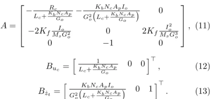
where, A is the 3×3 state matrix,Buc is the 3×1 input matrix, is the 3×1 disturbance matrix, andC is theα×3 output matrix (α varies from 1 to 5 (in this application), since its size changes according to the number of sensors in the sensor set). The aforementioned matrices are given by (11)–(13) in the Appendix. The various sensor sets can be obtained by appropriate selection of the corresponding rows in the output matrix C.
Note that the linearized model of the EMS is used for the design of the LQG controller, whereas for the tuning of the controller as well as for the validation via FIL, the non-linear model is applied in the loop.
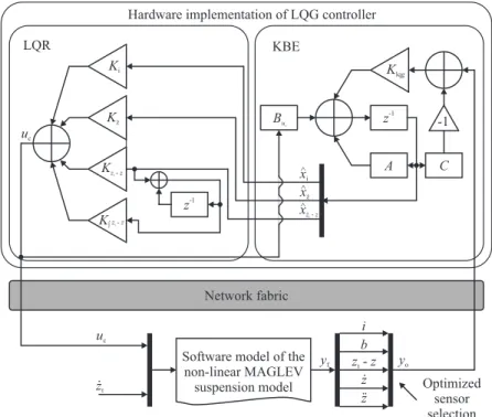
Network fabric yo C z-1 A Klqg -1
Software model of the non-linear MAGLEV suspension model yf uc z˙t i b z¨ ˙ z zt-z Ki zt-z K ˙ Kz K∫zt-z z-1 xi xz xzt-z ^ ^ ^ ˙ ˙ Buuc uc
Hardware implementation of LQG controller
LQR KBE
Optimized sensor selection Fig. 2.Optimized sensor selection framework validation using FIL
2.2 Closed-loop control requirements
The closed-loop design requirements for the EMS de-pend on the type and operating velocity of the train [14], and are affected by the magnitude of the input bances to the suspension. There are two types of distur-bances that enter in the vertical direction of the EMS:
(a) a stochastic behavior due to random variations of the rail position during vehicle movement;
(b) a deterministic behavior [4], considered in this work, occurs from the transition of the EMS onto the rail’s gradients.
With the total weight taken as 1000 kg, the operating point values for the EMS system are:Go= 0.015 m,Bo= 1 T, Io= 10 A, Vo= 100 V andFo= 9810 N. Hence, the parameters of the electromagnets, based on the operating point of the EMS, were calculated as follows:Rc= 10 Ω,
Lc = 0.1 H, Nc = 2000 and Ap = 0.01 m2. The deter-ministic disturbance here corresponds to a 5 % track gra-dient at a vehicle speed of 15 m/s, an acceleration equal to 0.5 m/s2, and a jerk (rate of change of acceleration) of 1 (m/s2)/s . The EMS must support the payload and follow the track gradients. As a result, there are specific boundaries where the EMS is allowed to operate: (i) max-imum airgap deviation, (zt−z)p≤7.5 mm; (ii) maximum control effort, ucp ≤ 300 V; (iii) settling time, ts ≤3 s, and (iv) airgap steady state error, e(zt−z)ss = 0 .
The control specifications are particularly addressed by the LQR controller in the first instance.
3 SYSTEMATIC FRAMEWORK FOR FIL
Any industrial plant has a number of control in-puts {ui: i = 1, . . . , nu}, input disturbances {di:i = 1, . . . , nd} and a set of possible outputs, ie, the full sen-sor set, Yf ={yi:i= 1, . . . , ns}. Part of the problem is to determine the set of sensors, Y ⊂ Yf, for which the system is (i) stable, (ii) satisfies a number of closed-loop performance criteria and (iii) has a minimum number of sensing elements in the selected set, ie, the number of elements in Yo is minimal1. The selection of Yo with respect to the aforementioned properties is a very impor-tant and complex process, especially if the plant has a large number of actuator/sensor configuration possibili-ties,ie, sets.
This work is focused upon optimized sensor selection with respect to the aforementioned three properties. The full sensor set Yo is a subset of the full sensor set Yf. Many subsets of the full sensor set are possible to be formed, and the number of them can be calculated from Ns= 2ns−1 , where Ns is the total number of all sensor sets and ns is the total number of sensors.
The LQG controller combines a linear quadratic regu-lator (LQR), and a Kalman filter (KBE). The controller tuning is done via the separation principle [5]; the frame-work algorithm is executed in two stages:
1
This paper deals only with minimizing the number of sensors, however there are other objectives that could be meaningful for applications other than the EMS systems. These can include mini-mizing energy consumption, size of weight and cost,etc.
(i) In the first step, the LQR controller is optimized using a GA and the Pareto-optimality between the two objective functions, (ie, φ1 = irms and φ2 = ¨zrms) is found. The LQR controller state feedback gains (ie, Klqr = hKi, Kz˙, K(zt−z), KR(zt−z)
i
, deduce the desired closed-loop response which is then selected and accounted as the desired or reference response for the next step.
(ii) The KBE is tuned for every feasible sensor set in order to achieve the desired closed-loop response.
Hence, a table is presented listing the optimised sensor sets with the selection of the “best” sensor set obtained by the overall control constraint violation function Ω. The latter is given by,
Ω k(l), f(j) = nk X l=1 ωl k(l)+ nf X j=1 ψj f(j) (3)
where ωl k(l), ψj f(j) are the lth, jth soft and hard control constraint violations respectively, nk and nf are the number of soft and hard control constraints, and Ω is a function where any control constraint violation is re-flected. If all control constraints are satisfied Ω becomes zero, otherwise its value depends on the level of the con-straint(s) violation.
Figure 2 illustrates the FIL applied on the EMS where all five outputs, Yf, out of which only the Yo (ie, the “best” sensor set) is fed into the FIL-based KBE.
4 FPGA–BASED ARCHITECTURE OF THE LQG CONTROLLER
The discrete linear time-invariant KBE has the follow-ing state space form,
˙ˆ x(k+ 1) =Adxˆ(k)+Bd ucuc(k)+K d lqg y(k)−Cdxˆ(k) , ˆ y(k) =Cdˆx(k) (4)
where ˆx are the estimated states, Kd
lqg is the 3×β observer gain matrix (β is the number of sensors) that minimizes E
[x−ˆx]⊤
[x−xˆ] (x represents the actual states). Ad,Bd
uc are the state and input matrices given by (14) and (15) in the Appendix. Kd
lqg has been calculated using the discrete time linear model of the EMS with a sampling rate of 10. Standard discretization procedure is followed here, hence full analysis is omitted.
The design architecture of the LQG core implemen-tation and its entity in very high speed integrated cir-cuits (VHSIC), hardware description language (VHDL) are depicted in Fig. 2 and Program 4 respectively. Fig-ure 2 illustrates the internal architectFig-ure of A3×3
block, while a similar design approach is followed for Cα×3
and Klqg3×β blocks. In the present work, we used the MATLAB HDL coder tool to automate and speed up the process of translating the high level simulation model into an equiv-alent register transfer level (RTL) HDL description. Due to MATLAB HDL coder limitations in handling multi dimension matrices, a detailed LQG core model using
B3 1x K u* z-1 xi xz x(zt- )z ^ ^ ^˙ z-1 z-1 K u* K u* +++ + + + + + + A3 3x C3 3x K u* K u* K u* K u* ++ z-1 K3 3x lqg + + + + + + + + + + uc uc Control input fixpt scaling airgap gain velocity gain current gain Sensor measurements y1 y2 y3 Estimated states uc A(1,1) A(2,1) A(3,1) A(1,2) A(2,2) A(3,2) A(1,3) A(2,3) A(3,3) + + + + + + + + + In1 In2 In3 Out2 Out1 Out3 (a) (b)
explicitly scalar buses (see Fig. 2 and Program 1) was developed prior to HDL translation.
4.1 Quantization process
An algorithm in a high level system modelling envi-ronment (such as MATLAB/Simulink) is represented in the floating-point domain, where mostly all variables are 64–bit allowing all operations to be performed in high precision format with large accuracy. In a digital VLSI implementation this translates to an increased number of flip-flops and combinational logic and inevitably results on a design that requires a large silicon area on the FPGA chip, large critical path that negatively affects speed, plus increased power consumption.
To address the aforementioned problem, the algorithm under implementation (LQG in this work) has first un-dergone a conversion to the fixed-point domain and then modelled using VHDL. In the fixed-point domain, a pair of wordlength, WL, and quality fractional range, QF, is considered for each parameter of the algorithm. As a consequence as (WL,QF) is increased will give a smaller Bit-Error Rate (BER) but larger silicon area, whereas as (WL,QF) is reduced will result to increased BER and smaller silicon area. Several simulations need to run to de-cide on the number of bits for (WL,QF) and the dynamic range of the parameters (MATLAB fixedpoint tool), in order to maintain a desired precision which will not com-promise the overall system performance (ie, destabilize the control loop), and maintain a low silicon area.
The fixed-point range for a signed number ±a in a 2’s complement form is defined by the minimum and maximum value range a signed integer number type of Quantity Integer range (QI) bits can hold. The latter is best expressed by the inequality, −2QI−1≤a≤2QI−1−1 and can be rewritten,
−2QI−1≤a <2QI−1, a∈
Z. (5)
From (5) it can be easily shown that,
QI|amin ≥log2(−a) + 1 ifa <0,
QI |amax >log2(a) + 1 ifa >0.
(6)
Since the positive constraint is the tighter one due to the asymmetry of signed integer types about zero, the con-straint for the required number of bits can be generalised as follows,
QI >log2 max[|amin|,|amax|]
+1. (7)
Since QI is an integer number of bits we can truncate the result and add one to form an equation to compute QI (that satisfies the constraint QI >log2|a|) such as,
QI=
log2 max[|amin|,|amax|]
+2
. (8)
2
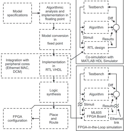
Each slice contains 4 Look Up Tables (LUTs) and 8 Flip-Flops (FFs). Model specifications Algorithmic analysis and implementation in floating point Model conversion in fixed point Implementation in RTL VHDL Integration with peripheral cores (Ethernet MAC, DCM) Logic synthesis Place and Route FPGA configuration Testbench Algorithm RTL design Testbench Algorithm ML605 FPGA Board Diff Diff Results Results Stimuli Stimuli Co-simulation with MATLAB HDL Simulator FPGA-in-the-Loop simulation Ethernet link
Assuming a resolution ε= 2−QF
for the fractional part, the qauantity fractional (QF) range becomes, QF = ⌈log(ε−1
)⌉; hence, the required wordlength W L, to suf-ficiently represent a float number to a fixed point repre-sentation, is given by the sum of QI and QF such that,
W L|Req≥QI +QF (9)
or
−2QI−1≤a <2QI−1−2−QF
|ε=2−QF . (10) 4.2 FPGA Implementation
The FIL presented in this work was implemented on a Xilinx Virtex-6 ML605 development board. The ML605 board utilizes a Xilinx Virtex-6 device (XC6VLX240T-1FFG1156) [15] in the 1156-pin fine-pitch Ball Grid Array (BGA) package, featuring slices2 and special Digital Sig-nal Processing (DSP) slices (DSP48A1). The LQG and the peripheral cores were synthesized using Xilinx Syn-thesis Tool (XST).
A top-down manner [16] has been followed for the design process of the LQG controller (Fig. 4). The pro-cess initiates with the model specifications and require-ments, advances to a high level functional system model (Simulink model) and continues on converting it to fixed-point prior to FPGA implementation. Co-simulation of the RTL model side-by-side with the fixed-point Simulink model was performed using MATLAB’s HDL verifier and Mentor’s Modelsim simulator in [17]. Moreover the im-plemented system on the FPGA chip was compared in real time using a cycle accurate Simulink model forming a FIL setup.
5 RESULTS ANALYSIS
In this section, the results from the FIL used to vali-date the sensor selection framework are analyzed. As ex-plained in Section 3, the first step in the output selec-tion process is to design the state vector Klqr. This is based on three performance criteria: (i) closed-loop ver-tical acceleration, ¨zrms <0.5 m/s2, (ii) excitation coil’s current, irms < 2 A and (iii) best possible ride quality,
ie, min ¨zrms
.
Note that the analysis related to Figs. 5, 6, 7, 8, is per-formed on the continuous-time [5] system to emphasize the design expectation aspects prior to implementation. This is not problematic as a sampling rate – for discreti-sation – of 10 kHz is used, which is well above the typical maglev loop bandwidth of < 20 Hz. The discrete time LQG controller is listed in the Appendix.
5.1 LQR Controller
Although the emphasis of the paper is the HIL em-bedded nature of the design, here we present some useful details on the design of the controller. In particular, the LQR controller is designed via the usual procedure of minimising the cost function Jlqr =
R
x⊤
Qx+u⊤ Ru
with the tuning matrices setup via Bryson’s rule [3]. We select LQR gains on the “best” (lowest value) ride quality level using nominal parameters for the model. Then the LQR design is assessed in terms of the robustness level by allowing ±10 % dynamic system parameter variation from nominal values for the following parameters: mass of vehicle (force follows trend), resistance and inductance, initial condition of current, initial condition of flux. The total combinations given the parameters is = 1125 . Fig-ure 5 illustrates the characteristic loci of the return ratio and CL poles. It is clearly shown that the ideal robust properties of LQR are not violated.
Figure 6 illustrates the magnitude spectrum of the closed-loop: vertical acceleration and air-gap, respec-tively, to ˙zt. The typical ride quality criterion of <5 %g RMS acceleration is not violated (note that deterministic responses are discussed later in this section).
5.2 Kalman filter (KBE) in the closed loop The KBE in the second step of the framework is used to estimate the states, thus an optimized tuning of the KBE is necessary to accurately estimate the states and feed the LQR controller.
Table 1. Optimized sensor selection simulation results
id SensorSet Deterministicresponse Ω
LQR response → X X 1 b X X 2 (zt−z) × × 3 z¨ X X 4 i, b X X 5 i,z¨ X X 6 i, b,(zt−z) X X 7 i, b,¨z X X 8 i, b,z,˙ z¨ X X 9 i, b,(zt−z),z,˙ z¨ X X
The optimization process shown that 24 out of 31 sen-sor sets provided the same closed-loop response (including the dynamic controller) compared to the closed-loop with the ideal LQR (the design was on the nominal system). Some of the corresponding results from the offline frame-work are presented in Table 1. The first column is the sensor set identification number (id), the second column is the corresponding sensor set, and the next two columns show whether the deterministic response of the EMS is satisfied (X) or not (×). The Ω function in the last col-umn similarly indicates whether all control constraints described in Section 2.2 are fulfilled (X) or not (×). The selection of the best sensor set is done based on Ω as described in Section 3. From a close inspection on the ta-ble, one can easily identify the best sensor set selection
ie, the one with the minimum number of sensor/s which satisfies all control requirements is id:1. In this work, the
-120 -40 0 Im Re 0 20 10 -10 -20 -80 -10 -1 0 Im Re 0 10 -6 0 5 -2 -4 -8
Fig. 5.LQR Robustness Return ratio and closed-loop poles,(tuning performed on nominal system ”best” ride quality) / continuous-time
103 0 -40 102 101 100 10-1 10-2 mag (dB) 0 40 f(rad/s) Fig. 6. CL responses with LQR only ( ˙zt → ¨z (top) and ˙z →
(z−zt) (bottom)) under model variation
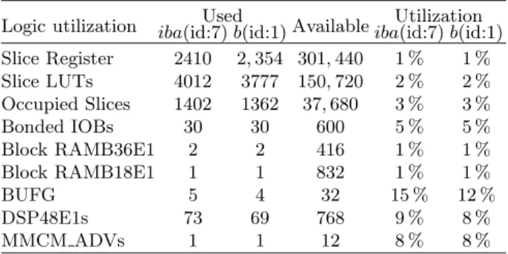
Table 2.Design utilization summary: three sensors, iba (id:7); and one sensor, b (id:1)
Logic utilization iba(id:7)Usedb(id:1)AvailableibaUtilization(id:7)b(id:1)
Slice Register 2410 2,354 301,440 1 % 1 % Slice LUTs 4012 3777 150,720 2 % 2 % Occupied Slices 1402 1362 37,680 3 % 3 % Bonded IOBs 30 30 600 5 % 5 % Block RAMB36E1 2 2 416 1 % 1 % Block RAMB18E1 1 1 832 1 % 1 % BUFG 5 4 32 15 % 12 % DSP48E1s 73 69 768 9 % 8 % MMCM ADVs 1 1 12 8 % 8 %
FIL was implemented for id:1 (single sensor), and is com-pared with id:7 (three sensors). The LQG-type controller,
ie, incorporating the Kalman filter and the LQR gains, implementation flow on the FPGA for other sensor set combinations follows the same approach.
Here we considered the design of the Kalman filter so as to provide the “best” estimates to the LQR con-troller. Some information on the impact of introducing
the Kalman filter –in the closed-loop – on preliminary ro-bustness performance (given the parameter variation con-sidered from the LQR design section) is also presented. As in the case of LQR only, we look into the stochastic ride quality criterion. Figure 7 shows the (continuous-time) magnitude spectrum of the closed-loop: vertical acceler-ation and air-gap, respectively, to ˙zt. Note that the KF considered in this set of figures is based on id:7 sensor set. Figure 8 shows the results on stochastic ride quality under parameter variation (CL with KF+LQR). The typ-ical criterion of <5 %g acceleration is not violated, with 90 % of the samples being less than 3.9 %g acceleration level.
5.3 FPGA implementation for 2 sensor sets The resources requirements and trial and error quan-tization procedure are commented in this section. Table 2 show the logic utilization for the implemented integrated system on the FPGA device, for three and one sensor.
103 0 -40 102 101 100 10-1 10-2 mag (dB) 0 40 f(rad/s) Fig. 7. CL responses with LQR+Kalman filter ( ˙zt→z¨(top) and
˙
zt→(z−zt) (bottom)) under model variation
2.4 2.8 3.2 3.6 4.4
Probability of ride quality samples being < projected value
Ride quality value (%g) 1.0 0.8 0.6 0.4 0.2 4.0 X:3.334 Y:0.5022 X:3.896 Y:0.9022
Fig. 8.Stochastic ride quality of CL with KF+LQR under param-eter variation – Cumulative distribution function plot (acceleration
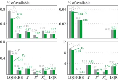
LQG 0.59 0.47 0.4 0.8 KBE Ad Bd Kd lqg LQR 0.11 0.10 0.15 0.15 0.07 0.02 0.15 0.09 0.11 0.11 y0 y1 LQG KBE Ad Bd Kd lqg LQR 0.13 0.13 3.523.52 1.82 0.781.04 1.56 2.99 2.99 y0 y1 9.51 8.98 4 12 8 % of available 0.54 0.4 0.8 0.13 0.12 0.19 0.170.09 0.02 0.21 0.120.12 0.12 y0 y1 0.74 % of available 0.03 0.02 0.010.01 y0 y1 0.04 0.02 0.04 0.04
Fig. 9.FPGA resources comparison for id:7 and id:1
6 6 4 2 0 ( - )zt ze(mx10 ) -4 6 time (s) 2 2 6 6 4 2 0 time (s) 2 i(A) 4 2 0.2 0.6 z(m/s) ( - )zt z (mx10 3 ) ˙ Current with LQR
Estimated current with FIL
Velocity with LQR
Estimated velocity with FIL
Airgap with LQR
Estimated airgap with FIL
(a)
(b)
Fig. 10. (a) — Airgap error with sets (id:1), (id:7) (b) — State estimation with set (id:1)
The implemented design mainly includes the LQG core, ethernet medium access control (MAC) [18] and the clock manager modules. The ethernet MAC core is licensed as part of the Xilinx embedded development kit
(EDK). According to the device utilization report from the Xilinx map (MAP) tool (see Table 3), the LQG core module itself for id:7, occupies 265 slices, 113 slice regis-ters, 884 slice LUTs, and 73 DSP cores (DSP48A1) and similarly for id:1, 205 slices, 111 slice registers, 696 slice LUTs, and 69 DSP48A1. A comparison of the utilized FPGA resources between three sensors, iba(set id:7) and one sensor, b (set id:1) LQG implementation scenarios, is depicted in Fig. 9. It is easy to see that the overall occupied area for set id:1 onto the FPGA chip is signifi-cantly smaller when compared to what is required by set id:7. The implemented design uses one mixed mode clock manager (MMCM) module [19] that produces the differ-ent clocks inside the FPGA chip. The placed and routed FPGA designs (LQG and peripheral cores) for three and one sensor implementations, achieve according to post-place and route timing report a system clock operating frequency of 34.364 ns or 29.1 MHz, and 32.819 ns or 30.5 MHz respectively. The aforementioned speeds were obtained with the map and place and route effort set to medium on Xilinx ISE 13.3.
5.4 Data analysis from FIL simulations
Figure 10 depicts the performance of the EMS us-ing two sensor sets. One comprisus-ing a sus-ingle sensor (set id:1) and the other one having three sensors (set: id:7). In particular, Fig. 10a compares the airgap deflection er-ror from simulation-based continuous-time and FIL-based discrete-time KBE with set id:1 (top) and set id:7 (bot-tom). The performance of the EMS is within the required performance objectives given in Section 2.2. The airgap error magnitude between the simulation and FIL is in the order of d-4 which is fairly small. The state estimation of the LQG using set id:1 is shown in Fig. 10b. All three states (i, ˙z and zt−z) are accurately estimated using one sensor (b), which has similar performance to the state estimation achieved with more sensors added,ie, set id:7. Hence, the EMS system can perform adequately, with re-spect to the given requirement, with fewer sensors.
6 CONCLUSIONS
A semi-practical modeling and validation of an em-bedded control system for sensor optimization on a EMS plant using the FIL concept was presented. A high-level MATLAB/Simulink environment used to model the phys-ical process and the LQG controller implemented on an FPGA. A model-based design approach has been followed for the FIL implementation using a fusion of system mod-eling and hardware/software co-design. Robustness issues on the LQR and designed LQG (i.e., Kalman-Filter and LQR) as well as the effect of fixed-point quantization was analyzed early in the design process. In the quantization case the wordlength was optimized to yield a smaller im-plementation. System level test benches were used with HDL co-simulation to verify the HDL implementation, and also FIL simulation to significantly accelerate the sys-tem validation. Without loss of generality, we compared FIL results for the LQG implementation of two sensor sets (id:1 and id:7). It was shown that the LQG imple-mentation in FIL is successful in spite of the complex quantization procedure.In addition it was shown that the FIL approach greatly reduces simulation time when com-pared to the software-based model counterpart. Current work studies design architecture of LQG with dynamic switching of the gains given the sensor set provision.
Table 3.Design utilization summary: three sensors,iba(id:7), and one sensor,b(id:1)
(a) id:7
Module (iba) Slices Slice reg. LUTs DSP48E1
LQG 0/265 0/113 0/884 0/73 KBE 49/221 77/77 170/717 1/50 Ad 67/67 0/0 221/221 27/27 Cd 30/30 0/0 99/99 14/14 Kd lqg 75/75 0/0 227/227 8/8 LQR 44/44 36/36 167/167 23/23 (b) id:1
Module (b) Slices Slice reg. LUTs DSP48E1
LQG 0/205 0/111 0/696 0/69 KBE 41/161 75/75 143/529 1/46 Ad 69/69 0/0 220/220 27/27 Cd 12/12 0/0 30/30 6/6 Kd lqg 39/39 0/0 136/136 12/12 LQR 44/44 36/36 167/167 23/23
N o t e . This paper is an extended version of earlier work presented by the authors in [20]. In particular, the authors extend their previous work by in-depth investi-gation of robustness, both in the design stage and expec-tations as well as in the robustness of the quantization (which works appropriately in both “worst” and “best” ride quality case choices).
Appendix A. EMS State space matrices (sym-bolic parameters) A= − Rc Lc+KbNcApGo − KbNcApIo G2 o Lc+KbNcApGo 0 −2KfMIsoG2 o 0 2Kf I2 o MsG3o 0 −1 0 , (11) Buc = h 1 Lc+KbNcApGo 0 0 i⊤ , (12) Bz˙t = h KbNcApIo G2 o Lc+KbNcApGo 0 1 i⊤ . (13)
While the output matrix C, for the different output mea-surements as mentioned in the main body of the paper, is formed by the relevant raw combination(s) from the state and input matrices accordingly.
Appendix B. LQG controller state-space ma-trices numerical results (relating to sensor sets, id:1 and id:7)
Ad= 9.99×10⁻¹ −6.34×10⁻² 4.15×10⁻³ 1.96×10⁻⁴ 1.00 −1.30×10⁻¹ −9.80×10⁻⁹−1.00×10⁻⁴ 1.00 , (14) Bduc= [ 4.76×10 −5 4.67×10⁻⁹ −1.55×10⁻¹³]⊤ , (15) Bd ˙ zt= [ 6.34×10 −2 −3.12×10⁻⁷ 1.00 ]⊤, (16) Kd lqg= 3.56×10⁻¹ −57.0 −2.82 −3.11×10⁻⁶ 1.49×10⁻³ 7.40×10⁻⁵ 5.61×10⁻⁴ −9.00×10⁻²−4.45×10⁻³ , (17) Cd= 1.00 0 0 0.10 0 −66.6 1.96 0 −1.30×10³ , (18) Kd lqg= [−1.61×10² 3.61×10 −3 −2.54×10⁻¹ ]⊤, (19) Cd = [ 0.10 0 −66.6 ]⊤. (20) References
[1] ISERMANN, R.—SCHAFFNIT, J.—SINSEL, S. : Hardware-in-the-Loop Simulation for the Design and Testing of Engine-Con-trol Systems, ConEngine-Con-trol Eng. Pract.7No. 5 (1999), 643–653. [2] LU, B.—WU, X.—FIGUEROA, H.—MONTI, A. : A Low-Cost
Real-Time Hardware-in-the-Loop Testing Approach of Power Electronics Controls, IEEE Trans. Ind. Electron. 54 No. 2 (2007), 919–931.
[3] MICHAIL, K.—ZOLOTAS, A.—GOODALL, R. M. : Opti-mised Configuration of Sensors for Fault Tolerant Control of an Electromagnetic Suspension System, Int. J. Syst. Sci.43No. 10 (2012), 1785–1804.
[4] MICHAIL, K. : Optimised Configuration of Sensing Elements for Control and Fault Tolerance Applied to an Electro-Magnetic Suspension System, 2009.
[5] SKOGESTAD, S.—POSTLETHWAITE, I. : Multivariable Feedback Control Analysis and Design, 2nd
edition, John Wiley & Sons Ltd, New York, 2005.
[6] KONAK, A.—COIT, D. W.—SMITH, A. E. : Multi-Objective Optimization using Genetic Algorithms: A Tutorial, Reliab. Eng Syst. Saf.91No. 9 (2006), 992–1007.
[7] ZHANG, Y.—JIANG, J. : Bibliographical Review on Reconfig-urable Fault-Tolerant Control Systems, Annu. Rev. Control32 No. 2 (2008), 229–252.
[8] BOUKHNIFER, M. : Active Fault Tolerant Control for Ul-trasonic Piezoelectric Motor, J. Electr. Eng. 63No. 4 (2012), 224–232.
[9] FORRAI, A. : Embedded Control System Design: A Model Based Approach, Springer Sci. & Business Media, 2012. [10] ALUR, R.—HRISTU-VARSAKELIS, D.—ARZEN,
K.-E.—LE-VINE, W.—BAILLIEUL, J.—HENZINGER, T. A. Eds. : Hand-book of Networked and Embedded Control Systems, Corr., 2nd
printing, Birkhauser, Boston, 2008.
[11] BACIC, M. : On Hardware-in-the-Loop Simulation, 4th
IEEE Conference on Decision and Control and European Control Con-ference, 2005, pp. 3194–3198.
[12] LUCIA, O.—JIMENEZ, O.—BARRAGAN, L. A.—URRIZA, I.—BURDIO, J. M.—NAVARRO, D. : Real-Time FPGA-based Hardware-in-the-Loop Development Test-Bench for Multiple Output Power Converters, in 6th
Annual IEEE Applied Power Electronics Conference and Exposition (APEC), 2010, 309–314. [13] DELIPARASCHOS, K. M.—MICHAIL, K.—TZAFESTAS, S. G.—ZOLOTAS, A. C. : Optimised Sensor Selection for Con-trol: A Hardware-in-the-Loop Realization on FPGA for an EMS System, in Conference on Control and Fault-Tolerant Systems (SysTol), 2013, pp. 727–732.
[14] GOODALL, R. M. : Dynamics and Control Requirements for EMS Maglev Suspensions, in Proceedings on International Con-ference on Maglev, 2004, pp. 926–934.
[15] Xilinx Inc., Virtex-6 Family Overview. 2012.
[16] DELIPARASCHOS, K. M.—NENEDAKIS, F. I.—TZAFES-TAS, S. G. : Design and Implementation of a Fast Digital Fuzzy Logic Controller using FPGA Technology, J. Intell. Robot. Syst. 45No. 1 (Jan 2006), 77–96.
[17] MOUSTRIS, G. P.—DELIPARASCHOS, K. M.—TZAFES-TAS, S. G. : Feedback Equivalence and Control of Mobile Robots through a Scalabe FPGA Architecture, in Recent Ad-vances in Mobile Robotics (Dr. Andon Venelinov Topalov, ed.), InTech, 2011.
[18] Xilinx Inc., LogiCORE IP Virtex-6 FPGA Embedded Tri-Mode Ethernet MAC Wrapper v2.3. 2012.
[19] Xilinx Inc., Virtex-6 FPGA Clocking Resources User Guide. 2014.
[20] DELIPARASCHOS, K. M.—MICHAIL, K.—TZAFESTAS, S. G.—ZOLOTAS, A. C. : A Model-Based Embedded Control Hardware/Software Co-Design Approach for Optimized Sensor Selection of Industrial Systems, in 23th
Mediterranean Confer-ence on Control and Automation (MED), Toremolinos, Spain, 2015, pp. 889–894.
Received 17 January 2016
Kyriakos M. Deliparaschosborn in Athens, Greece, re-ceived his BEng Hons degree in Electronics Engineering from De Montfort University, Leicester, UK, the MSc degree in Mechatronics from De Montfort University and National Tech-nical University of Athens (NTUA), and his PhD degree from the Department of Signals, Control and Robotics, School of Electrical and Computer Engineering, NTUA. Currently he is Adjunct Lecturer at the Department of Electrical and Com-puter Engineering and Informatics of Cyprus University of Technology (CUT), a Research Associate with the Robotics Control and Decision Systems (RCDS) Lab part of the Me-chanical Engineering and Material Science and Engineering
Department of the CUT, and also a Research Associate at the Intelligent Robotics and Automation Lab of NTUA. Pre-viously he was a Postdoctoral Research Fellow (DISCUS FP7 funded project,) with CTVR group at Trinity College, Dublin University.
Konstantinos Michailwas born in Nicosia, Cyprus. He obtained his BSc in Electronic Engineering from Budapest University of Technology and Economics, Hungary, 2003. In 2004 he received an MSc from Newcastle University Upon Tyne, UK and in 2009 he was awarded the PhD degree from Loughborough University, UK both in automatic control sys-tems. His research activities fall in the areas of modern and classical control methods, robust control, fault tolerant con-trol, multi-objective optimization, renewable energy systems, communication systems, robotics and digital signal process-ing. He has published a number of journal and conferences papers in control systems. Since 2013 he is a senior research engineer with SignalGeneriX Ltd working on communications and control systems R&D.
Argyrios C. Zolotas, born in Xanthi, Greece, graduated from the University of Leeds in 1998 and received his PhD degree in 2002 from Loughborough University. He also ob-tained an MSc (Distinction) from University of Leicester via a part-time program under the lifelong learning initiative of the LLP-CPD framework. Since September 2014 he is Reader (and from January 2015 also deputy director of research) in the School of Engineering, University of Lincoln UK. He pre-viously held academic positions at University of Sussex and Loughborough University, and a post-doctoral research fellow-ship at Imperial College London. He is senior member of the IEEE and a fellow of the UK Higher Education Academy. His research interests are in the areas of robust control of lin-ear and nonlinlin-ear systems, system structure selection, system resilience, applications of advanced control, emerging control applications.
Spyros G. Tzafestaswas born in Corfu, Greece. He holds PhD and DSc degrees in Control and Automation and he is professor emeritus, Director of the Institute of Communica-tion and Computer Systems (ICCS), senior research associate of the Signals, Control and Robotics Division and the Intel-ligent Robotics and Automation Laboratory (IRAL) of the National Technical University of Athens (NTUA). He is recip-ient of honorary doctorates from the International University (DSc (Hon)), the Technical University of Munich (Dr-Ing Eh) and the Ecole Centralede Lille (Docteur Honoris Causa). Fel-low of IEEE (N.Y.) and IEE (London); Member of ASME (N.Y.), New York Academy of Sciences, IMACS (Rutgers, N.J.) and SIRES (Brussels). Member of IFAC SECOM and MIM TCs. Project evaluator of national European and inter-national projects (USA, Canada, Italy, Hong Kong, Japan). Project coordinator of national and EU projects in the fields of robotics, CIM and IT (ESPRIT, BRITE-EURAM, TIDE, INTAS, SOCRATES, EUREKA, GROWTH, etc.). Publica-tions: 30 research books, 60 book chapters, over 700 journal and conference technical papers. Editor-in Chief of the Journal of Intelligent and Robotic Systems (1988–2005) and the book series “Microprocessor-Based and Intelligent Systems Engi-neering” (K1uwer). Organizer of several international
confer-ences (IEEE, IFAC, IMACS, IASTED, SIRES etc). Listed in
several international biographical volumes. Current interests include: control, robotics and CIM.