Forthcoming in theJournal of Econometrics
Benchmark Priors
for Bayesian Model Averaging
Carmen Fern´andezSchool of Mathematics and Statistics, University of St. Andrews, St. Andrews KY16 9SS, U.K.
Eduardo Ley
International Monetary Fund, 700 19th St NW, Washington DC 20431, U.S.A.
Mark F. J. Steel
Institute of Mathematics and Statistics, University of Kent at Canterbury, Canterbury CT2 7NF, U.K.
Abstract. In contrast to a posterior analysis given a particular sampling model, posterior model probabilities in the context of model uncertainty are typically rather sensitive to the specification of the prior. In particular, “diffuse” priors on model-specific parameters can lead to quite unexpected consequences. Here we focus on the practically relevant situation where we need to entertain a (large) number of sampling models and we have (or wish to use) little or no subjective prior information. We aim at providing an “automatic” or “benchmark” prior structure that can be used in such cases. We focus on the Normal linear regression model with uncertainty in the choice of regressors. We propose a partly noninformative prior structure related to a Natural Conjugateg-prior specification, where the amount of subjective information requested from the user is limited to the choice of a single scalar hyperparameterg0j. The consequences of different choices forg0jare examined. We investigate
theoretical properties, such as consistency of the implied Bayesian procedure. Links with classical information criteria are provided. More importantly, we examine the finite sample implications of several choices ofg0jin a simulation study. The use
of the MC3algorithm of Madigan and York (1995), combined with efficient coding in Fortran, makes it feasible to conduct large simulations. In addition to posterior criteria, we shall also compare the predictive performance of different priors. A classic example concerning the economics of crime will also be provided and contrasted with results in the literature. The main findings of the paper will lead us to propose a “benchmark” prior specification in a linear regression context with model uncertainty.
Keywords.Bayes factors, Markov chain Monte Carlo, Posterior odds, Prior elicitation
JEL Classification System. C11, C15
The issue of model uncertainty has permeated the econometrics and statistics literature for decades. An enormous volume of references can be cited (only a fraction of which is mentioned in this paper), and special
issues of the Journal of Econometrics (1981, Vol.16, No.1) and Statistica Sinica (1997, Vol.7, No.2) are
merely two examples of the amount of interest this topic has generated in the literature. From a Bayesian perspective, dealing with model uncertainty is conceptually straightforward: the model is treated as a further parameter which lies in the set of models entertained (the model space). A prior now needs to be specified for the parameters within each model as well as for the models themselves, and Bayesian inference can be
conducted in the usual way, with one level (the prior on the model space) added to the hierarchy —see,e.g.,
Draper (1995) and the ensueing discussion. Unfortunately, the influence of the prior distribution, which is often straightforward to assess for inference given the model, is much harder to identify for posterior model
probabilities. It is acknowledged —e.g., Kass and Raftery (1995), George (1999)— that posterior model
probabilities can be quite sensitive to the specification of the prior distribution.
In this paper, we consider a particular instance of model uncertainty, namely uncertainty about which
variables should be included in a linear regression problem withk available regressors. A model here will
We thank Arnold Zellner, Dennis Lindley and two anonymous referees for their useful suggestions. Carmen Fern´andez gratefully acknowledges financial support from a Training and Mobility of Researchers grant awarded by the European Com-mission (ERBFMBICT # 961021). Carmen Fern´andez and Mark Steel were affiliated to CentER and the Department of Econometrics, Tilburg University, The Netherlands, and Eduardo Ley was at FEDEA, Madrid, Spain during the early stages of the work on this paper. Some of this research was done when Carmen Fern´andez was at the Department of Mathematics, University of Bristol, and Mark Steel at the Department of Economics, University of Edinburgh.
be identified by the set of regressors that it includes and, thus, the model space consists of 2k elements.1
Given the issue of sensitivity to the prior distribution alluded to above, the choice of prior is quite delicate, especially in the absence of substantial prior knowledge. Our aim here is to come up with a prior distribution that leads to sensible results, in the sense that data information dominates prior assumptions. Whereas we acknowledge the merits of using substantive prior information whenever available, we shall be concerned with providing the applied researcher with a “benchmark” method for conducting inference in situations where incorporating such information into the analysis is deemed impossible, impractical or undesired. In addition, this provides a useful backdrop against which results arising from Bayesian analyses with informative priors could be contrasted.
We will focus on Bayesian model averaging (BMA), rather than on selecting a single model. BMA follows directly from the application of Bayes’ theorem in the hierarchical model described in the first paragraph, which implies mixing over models using the posterior model probabilities as weights. This is very reasonable as it allows for propagation of model uncertainty into the posterior distribution and leads to more sensible uncertainty bands. From a decision-theory point of view, Min and Zellner (1993) show that such mixing over models minimizes expected predictive squared error loss, provided the set of models under consideration is exhaustive. Raftery, Madigan and Hoeting (1997) state that BMA is optimal if predictive ability is measured by a logarithmic scoring rule. The latter result also follows from Bernardo (1979), who shows that the usual posterior distribution leads to maximal expected utility under a logarithmic proper utility function. Such a utility function was argued by Bernardo (1979) to be “often the more appropriate description for the preferences of a scientist facing an inference problem”. Thus, in the context of model uncertainty, the use of BMA follows from sensible utility considerations. This is the scenario that we will focus on. However, our results should also be useful under other utility structures that lead to decisions different from model
averaging —e.g. model selection. This is because the posterior model probabilities will intervene in the
evaluation of posterior expected utility. Thus, finding a prior distribution that leads to sensible results in the absence of substantive prior information is relevant in either setting.
Broadly speaking, we can distinguish three strands of related literature in the context of model uncertainty. Firstly, we mention the fundamentally oriented statistics and econometrics literature on prior elicitation and model selection or model averaging, such as exemplified in Box (1980), Zellner and Siow (1980), Draper (1995) and Phillips (1995) and the discussions of these papers. Secondly, there is the recent statistics literature on computational aspects. Markov chain Monte Carlo methods are proposed in George and McCulloch (1993),
Madigan and York (1995), Geweke (1996) and Rafteryet al.(1997), while Laplace approximations are found
in Gelfand and Dey (1994) and Raftery (1996). Finally, there exists a large literature on information criteria,
often in the context of time series, see,e.g., Hannan and Quinn (1979), Akaike (1981), Atkinson (1981), Chow
(1981) and Foster and George (1994). This paper provides a unifying framework in which these three areas of research will be discussed.
In line with the bulk of the literature, the context of this paper will be Normal linear regression with uncertainty in the choice of regressors. We abstract from any other issue of model specification. We present a prior structure that can reasonably be used in cases where we have (or wish to use) little prior information,
partly based on improper priors for parameters that are common to all models, and partly on a g-prior
structure as in Zellner (1986). The prior is not in the natural-conjugate class, but is such that marginal likelihoods can still be computed analytically. This allows for a simple treatment of potentially very large
model spaces through Markov chain Monte Carlo model composition (MC3) as introduced in Madigan and
York (1995). In contrast to some of the priors proposed in the literature, the prior we propose leads to valid
conditioning in the posterior distribution (i.e., the latter can be interpreted as a conditional distribution given
the observables) as it avoids dependence on the values of the response variable. The only hyperparameter
left to elicit in our prior is a scalar g0j for each of the models considered. Theoretical properties, such
as consistency of posterior model probabilities, are linked to functional dependencies ofg0j on sample size
and the number of regressors in the corresponding model. In addition (and perhaps more importantly), we
conduct an empirical investigation through simulation. This will allow us to suggest specific choices forg0j
to the applied user. As we have conducted a large simulation study, efficient coding was required. This code
1 Of course, more models arise if we consider other aspects of model specification, but this will not be addressed here. See, e.g., Hoeting, Raftery and Madigan (1995, 1996) for treatments of variable transformations and outliers, respectively.
(in Fortran-77) has been made publicly available on the World Wide Web.2
Section 1 introduces the Bayesian model and the practice of Bayesian model averaging. The prior structure is explained in detail in Section 2, where expressions for Bayes factors are also given. The setup of the empirical simulation experiment is described in Section 3, while results are provided in the next section. Section 5 presents an illustrative example using the economic model of crime from Ehrlich (1973, 1975), and Section 6 gives some concluding remarks and practical recommendations. The Appendix presents results about asymptotic behaviour of Bayes factors.
1. THE MODEL AND BAYESIAN MODEL AVERAGING
We consider n independent replications from a linear regression model with an intercept, say α, and k
possible regression coefficients grouped in ak-dimensional vectorβ. We denote byZ the correspondingn×k
design matrix and we assume thatr(ιn :Z) =k+ 1, wherer(·) indicates the rank of a matrix and ιn is an
n-dimensional vector of 1’s.
This gives rise to 2k possible sampling models, depending on whether we include or exclude each of the
regressors. In line with the bulk of the literature in this area —see, e.g., Mitchell and Beauchamp, 1988,
George and McCulloch, 1993 and Rafteryet al., 1997—, exclusion of a regressor means that the corresponding
element ofβ is zero. Thus, a model Mj,j= 1, . . . ,2k, contains 0≤kj≤k regressors and is defined by
y=αιn+Zjβj+σε, (1.1)
where y ∈ <n is the vector of observations. In (1.1), Z
j denotes the n×kj submatrix of Z of relevant
regressors, βj ∈ <kj groups the corresponding regression coefficients and σ ∈ <+ is a scale parameter.
Furthermore, we shall assume that ε follows an n-dimensional Normal distribution with zero mean and
identity covariance matrix.
We now need to specify a prior distribution for the parameters in (1.1). This distribution will be given through a density function
p(α, βj, σ | Mj). (1.2)
In Section 2, we shall consider specific choices for the density in (1.2) and examine the resulting Bayes
factors. We group the zero components ofβ under Mj in a vectorβ∼j ∈ <k−kj,i.e.,
Pβ∼j|α,βj,σ,Mj =Pβ∼j|Mj = Dirac at (0, . . . ,0). (1.3)
We denote the space of all 2k possible models byM, thus
M={Mj:j= 1, . . . ,2k}. (1.4) In a Bayesian framework, dealing with model uncertainty is, theoretically, perfectly straightforward: we
simply need to put a prior distribution over the model spaceM
P(Mj) =pj, j= 1, . . . ,2k, withpj >0 and 2k
X
j=1
pj= 1. (1.5)
Thus, we can think of the model in (1.1)-(1.5) as the usual linear regression model where all possible regressors
are included, but where the prior onβ has a mixed structure, with a continuous part and a discrete point
mass at zero for each element. In other words, the model indexMj really indicates that certain elements of
β (namelyβ∼j) are set to zero, and, as discussed in Poirier (1985), we always condition on the full set of
available regressors.
2 Our programs, which can be found at mcmcmc.freeyellow.com should be slightly adapted before they can be used in other
problems. More flexible software to implement the approach in Smith and Kohn (1996) can be found at www.agsm.unsw.edu.au/
∼mikes, whereas the BMA webpage of Chris Volinsky at www.research.att.com/∼volinsky/bma.html lists various resources of relevance to BMA.
With this setup, the posterior distribution of any quantity of interest, say ∆, is a mixture of the posterior distributions of that quantity under each of the models with mixing probabilities given by the posterior model probabilities. Thus
P∆|y= 2k
X
j=1
P∆|y,MjP(Mj | y), (1.6) provided ∆ has a common interpretation across models. This procedure, which is typically referred to as Bayesian model averaging (BMA), is in fact the standard Bayesian solution under model uncertainty, since
it follows from direct application of Bayes’ theorem to the model in (1.1)–(1.5) —see,e.g., Leamer (1978),
Min and Zellner (1993), Osiewalski and Steel (1993) and Rafteryet al.(1997).
Posterior model probabilities are given by
P(Mj | y) = ly(Mj)P(Mj) P2k h=1ly(Mh)P(Mh) = 2 k X h=1 P(Mh) P(Mj) ly(Mh) ly(Mj) −1 , (1.7)
wherely(Mj), the marginal likelihood of modelMj, is obtained as
ly(Mj) =
Z
p(y | α, βj, σ, Mj)p(α, βj, σ | Mj)dαdβjdσ, (1.8) withp(y | α, βj, σ, Mj) andp(α, βj, σ | Mj) defined through (1.1) and (1.2), respectively.
Two difficult questions here are how to computeP(Mj | y) and how to assess the influence of our prior
assumptions on the latter quantity. Substantial research effort has gone into examining each of them:
In cases wherely(Mj) can be derived analytically, the computation ofP(Mj | y) is, in theory,
straight-forward, through direct application of (1.7). However, the large number of terms (2k) involved in the latter
expression often makes this computation practically infeasible. A common approach is to resort to an MCMC
algorithm, by which we generate draws from a Markov chain on the model spaceMwith the posterior model
distribution as its stationary distribution. An estimate of (1.7) is then constructed on the basis of the models
visited by the chain. An important example of this is the MC3 methodology of Madigan and York (1995),
which uses a Metropolis-Hastings updating scheme —see,e.g., Chib and Greenberg (1995). MC3was
imple-mented in the context of BMA in linear regression models by Rafteryet al. (1997), who consider a natural
conjugate prior structure in (1.2). The latter paper also proposes an application of the Occam’s window algorithm of Madigan and Raftery (1994) for deterministically finding the models whose posterior probability
is above a certain threshold. Under ag-prior distribution for the regression coefficients, the use of the fast
updating scheme of Smith and Kohn (1996) in combination with the Gray code order, allows for exhaustive
evaluation of all 2k terms in (1.7) whenkis less than about 25 —see George and McCulloch (1997).
Computing P(Mj|y) is a more complex problem when analytical evaluation of ly(Mj) is not available.
In that case, the reversible jump methodology of Green (1995), which extends usual Metropolis-Hastings methods to spaces of variable dimension, could be applied to construct a Markov chain jointly over parameter and model space. An alternative approach was proposed by George and McCulloch (1993), who instead of zero restrictions in (1.3), assume a continuous prior distribution concentrated around zero for these coefficients. In this way, they get around the problem of a parameter space of varying dimension and are still able to propose a Gibbs sampling algorithm to generate a Markov chain. Their approach is based on
a zero-mean Normal prior for β given Mj, where large and small variances are respectively allocated to
regression coefficients included in and “excluded” from Mj. Thus, they are required to choose two prior
variances, and results are typically quite sensitive to this choice. As the ratio of the variances becomes large, the mixing of the chain will often be quite slow. An alternative Gibbs sampler that can deal with prior point mass at zero and displays better mixing behaviour was proposed in Geweke (1996). A deterministic approach in the vein of Occam’s window was taken by Volinsky, Madigan, Raftery and Kronmal (1997), who
approximate the value ofly(Mj) and use a modified leaps-and-bounds algorithm to find the set of models to
average over (i.e., the models with highest posterior probability).
Apart from purely computational aspects, just described, the issue of choosing a “sensible” prior
by the prior odds [P(Mh)/P(Mj)] and the Bayes factors [Bhj ≡ly(Mh)/ly(Mj)] of each of the entertained
models versusMj. Bayes factors are known to be rather sensitive to the choice of the prior distributions for
the parameters within each model. Even asymptotically, the influence of this distribution does not vanish
—see, e.g., Kass and Raftery (1995) and George (1999). Thus, under little (or absence of) prior
informa-tion, the choice of the distribution in (1.2) is a very thorny question. Furthermore, the usual recourse to improper “non-informative” priors does not work in this situation, since improper priors can not be used for model-specific parameters [attempts to overcome this include the explicit or implicit use of training
sam-ples, using, e.g., intrinsic Bayes factors as in Berger and Pericchi (1996) or fractional Bayes factors as in
O’Hagan (1995), which, although conceptually quite interesting, suffer from a number of inconsistencies]. As a consequence, most of the literature has focussed on “weakly-informative” proper priors, which are often
data-dependent through the response variable —as the prior in, e.g., Raftery et al. (1997). George and
Foster (1997) propose an empirical Bayes approach (in a case with knownσ) to elicit prior hyperparameters,
in order to avoid the computational difficulties of a full Bayesian analysis with a further level of hierarchy. Whilst we do not wish to detract from the potential usefulness of data-dependent priors in certain contexts, we note that they do not allow for valid conditioning, in the sense that the posterior distribution can not be interpreted as a conditional distribution given the observables (although the hope, of course, is that the product of likelihood and “prior” still constitutes a suitable basis for inference in such cases). Here, we focus on priors that avoid dependence on the values of the response variable and, thus, avoid this (in our view, undesirable) property. We will propose certain priors and study their behaviour in comparison with other priors previously considered in the literature.
As a final remark before concluding this section, we note that, in line with the majority of recent Bayesian literature in this area, we consider a prior distribution that allows for the actual exclusion of regressors from some of the models —see (1.3). For us, the rationale behind this choice is that, when faced with a modelling scenario with uncertainty in the choice of covariates, the researcher will often ask herself questions of the form “Does the exclusion of certain subsets of regressors lead to a sensible model?”, thus interpreting the exclusion of regressors not like a dogmatic belief that such regressors have no influence whatsoever on the outcome of the process being modelled but, rather, as capturing the idea that the model which excludes those regressors is a sensible one. Just how sensible a model is will be quantified by its posterior probability, which combines prior information (or lack of it) with data information via Bayes’ theorem. Of course, there
might be situations in which utility considerations —e.g., cost of collecting regressors versus their predictive
ability, or some other consideration specific to that particular problem— dictate that certain regressors be dropped from the model even if their inclusion is sensible by the criterion mentioned above. In such cases, the use of a continuous prior concentrated around zero —as in George and McCulloch (1993)— instead of
(1.3) or, as a Referee suggested, conducting continuous inference about the full vectorβ followed by removal
of regressors according to utility considerations, could be preferable. However this paper will not consider design issues and, as mentioned in the Introduction, focusses on the case where neither substantive prior information nor a problem-specific decision theory framework are available, rendering our approach more natural. For more comments on the issue of discrete versus continuous priors, see Raftery, Madigan and Volinsky (1996) and the ensueing discussion.
2. PRIORS FOR MODEL PARAMETERS AND THE CORRESPONDING BAYES FACTORS
In this section, we present several priors —i.e., several choices for the density in (1.2)— and derive the
expressions of the resulting Bayes factors. In the sequel of the paper, we shall examine the properties (both finite-sample and asymptotic) of the Bayes factors.
2.1. A natural conjugate framework
Both for reasons of computational simplicity and for the interpretability of theoretical results, the most obvious choice for the prior distribution of the parameters is a natural conjugate one. The density in (1.2) is then given through
p(α, βj | σ, Mj) =fNkj+1((α, βj) | m0j, σ2V0j), (2.1)
σ2V
0j, and through
p(σ−2 | Mj) =p(σ−2) =fG(σ−2 | c0, d0), (2.2)
which corresponds to a Gamma distribution with mean c0/d0 and variancec0/d02 for σ−2. Clearly m0j ∈
<kj+1,V
0ja (kj+1)×(kj+1) positive definite symmetric matrix,c0>0 andd0>0 are prior hyperparameters
that still need to be elicited.
This natural conjugate framework greatly facilitates the computation of posterior distributions and Bayes
factors. In particular, the marginal likelihood of modelMj computed through (1.8) takes the form
ly(Mj) =fSn µ y | 2c0, Xjm0j, c0 d0 (In−XjV∗jXj0) ¶ , (2.3) where Xj= (ιn :Zj), (2.4) V∗j= (Xj0Xj+V0−j1)−1, (2.5) and fn
S(y | ν, b, A) denotes the p.d.f. of an n-variate Student-t distribution with ν degrees of freedom,
location vectorb(the mean ifν >1) and precision matrixA(with covariance matrixA−1ν/(ν−2) provided
ν >2) evaluated at y. The Bayes factor for model Mj versus model Ms now takes the form
Bjs= ly(Mj) ly(Ms) = µ |V∗j| |V0j| |V0s| |V∗s| ¶1/2( 2d0+ (y−Xsm0s)0(In−XsV∗sXs0)(y−Xsm0s) 2d0+ (y−Xjm0j)0(In−XjV∗jXj0)(y−Xjm0j) )c0+n2 . (2.6)
Generally, the choice of the prior hyperparameters in (2.1)–(2.2) is not a trivial one. The user is plagued by the pitfalls described in Richard (1973), arising if we wish to combine a fixed quantity of subjective
prior information on the regression coefficients with little prior information onσ. Richard and Steel (1988,
App. D) and Bauwens (1991) propose a subjective elicitation procedure for the precision parameter based on the expected fit of the model. See Poirier (1996) for related ideas. In this paper we shall follow the opposite strategy, and instead of trying to elicit more prior information in a situation of incomplete prior specification, we focus on situations where we have (or wish to use) as little subjective prior knowledge as possible.
2.2. Choosing prior hyperparameters for(α, βj)
Choosingm0jandV0j can be quite difficult in the absence of prior information. A predictive way of eliciting
m0j is through making a prior guess for then-dimensional response y. Laud and Ibrahim (1996) propose
to make such a guess, call itη, taking the information on all the covariates into account and subsequently
choose m0j = (Xj0Xj)−1Xj0η. Our approach is similar in spirit but much simpler: Given that we do not
possess a lot of prior information, we consider it very difficult to make a prior guess fornobservations taking
the covariates for each of these nobservations into account. Especially whenn is large, this seems like an
extremely demanding task. Instead, one could hope to have an idea of the central values ofyand make the
following prior prediction guess: η=m1ιn, which corresponds to
m0j = (m1,0, . . . ,0)0. (2.7)
Eliciting prior correlations is even more difficult. We adopt the convenient g-prior (Zellner 1986), which
corresponds to taking
V0−j1=g0jXj0Xj, (2.8)
with g0j > 0. From (2.5) it is clear that V0−j1 is the prior counterpart of Xj0Xj and, thus, (2.8) implies
that the prior precision is a fractiong0j of the precision arising from the sample. This choice is extremely
popular, and has been considered, among others by Poirier (1985) and Laud and Ibrahim (1995, 1996). See also Smith and Spiegelhalter (1980) for a closely related idea.
With these hyperparameter choices, the Bayes factor in (2.6) can be written in the following intuitively interpretable way Bjs= µ g0j g0j+ 1 ¶kj+1 2 µg 0s+ 1 g0s ¶ks+1 2 Ã 2d0+g0s1+1y0MXsy+g0gs0+1s (y−m1ιn)0(y−m1ιn) 2d0+g0j1+1y0MXjy+g0gj0+1j (y−m1ιn)0(y−m1ιn) !c0+n2 , (2.9) where y0MXjy=y0y−y0Xj(Xj0Xj)−1Xj0y (2.10)
is the usual Sum of Squared Residuals under modelMj.
Note that the last factor in (2.9) contains a convex combination between the model “lack of fit” (measured
throughy0MXjy) and the “error of our prior prediction guess” [measured through (y−m1ιn)0(y−m1ιn)].
The coefficients of this convex combination are determined by the choice ofg0j. The choice ofg0j is crucial
for obtaining sensible results, as we shall see later. By not choosing g0j through fixing a marginal prior of
the regression coefficients, we avoid the natural conjugate pitfall alluded to at the end of Subsection 2.1.
In addition, the g-prior in (2.7)-(2.8) can also lead to a prior that is continuously induced across models,
as defined in Poirier (1985), in the sense that the priors for all 2k models can be derived as the relevant
conditionals from the prior of the full model (withkj =k). This will hold as long asg0j does not depend on
Mj and we modify the prior in (2.2) so that the shape parameterc0 becomes model-specific and is replaced
byc0+ (k−kj)/2.
2.3. A non-informative prior forσ
From (2.9) it is clear that the choice ofd0, the precision parameter in the Gamma prior distribution forσ−2,
can crucially affect the Bayes factor. In particular, if the value ofd0is large in relation to the values ofy0MXjy
and (y−m1ιn)0(y−m1ιn) the prior will dominate the sample information, which is a rather undesirable
property. The impact ofd0on the Bayes factor also clearly depends on the units of measurement for the data
y. In the absence of (or under little) prior information, it is very difficult to choose this hyperparameter value
without using the data if we do not want to risk choosing it too large. Even using prior ideas about fit does
not help; Poirier (1996) shows that the population analog of the coefficient of determination (R2) does not
have any prior dependence onc0 ord0. Use of the information in the response variable was proposed,e.g.,
by Raftery (1996) and Rafteryet al.(1997) but, as we already mentioned, we prefer to avoid this situation.
Instead we propose the following:
Since the scale parameterσappears in all the models entertained, we can use the improper prior
distri-bution with density
p(σ)∝σ−1, (2.11)
which is the widely accepted non-informative prior distribution for scale parameters. Note that we have
assumed a common prior distribution forσ across models. This practice is often followed in the literature
—see e.g., Mitchell and Beauchamp, 1988, and Raftery et al., 1997— and leads to procedures with good
operating characteristics. It is easy to check that the improper prior in (2.11) results in a proper posterior
(and thus allows for a Bayesian analysis) as long asy6=m1ιn.
The distribution in (2.11) is the only one that is invariant under scale transformations (induced by,e.g., a
change in the units of measurement) and is the limiting distribution of the Gamma conjugate prior in (2.2)
when bothd0 andc0 tend to zero. This leads to the Bayes factor
Bjs= µ g0j g0j+ 1 ¶kj+1 2 µg 0s+ 1 g0s ¶ks+1 2 Ã 1 g0s+1y 0M Xsy+g0gs0+1s (y−m1ιn)0(y−m1ιn) 1 g0j+1y 0MXjy+ g0j g0j+1(y−m1ιn) 0(y−m1ιn) !n 2 , (2.12)
2.4. A non-informative prior for the intercept
In (2.12) there are two subjective elements that still remain, namely the choices of g0j and of m1, where
m1ιn is our prior guess for y. It is clear from (2.12) that the choice ofm1can have a non-negligible impact
on the actual Bayes factor and, under absence of prior information, it is extremely difficult to successfully
elicitm1 without using the data. The idea that we propose here is in line with our solution for the prior
onσ: since all the models have an intercept, take the usual non-informative improper prior for a location
parameter with constant density. This avoids the difficult issue of choosing a value form1.
This setup takes us outside the natural conjugate framework, since our prior for (α, βj) no longer
corre-sponds to (2.1). Without loss of generality, we assume that
ι0nZ = 0, (2.13)
so that the intercept is orthogonal to all the regressors. This is immediately achieved by subtracting the corresponding mean from each of them. Such a transformation only affects the interpretation of the intercept
α, which is typically not of primary interest. In addition, the prior that we next propose forαis not affected
by this transformation. We now consider the following prior density for (α, βj):
p(α)∝1, (2.14)
p(βj | σ, Mj) =f kj
N(βj | 0, σ2(g0jZj0Zj)−1). (2.15)
Through (2.14)–(2.15) we assume the same prior distribution for α in all of the models and a g-prior
distribution for βj under model Mj. We again use the non-informative prior described in (2.11) for σ.
Existence of a proper posterior distribution is now achieved as long as the sample contains at least two
different observations. The Bayes factor forMj versusMs now is
Bjs= µ g0j g0j+ 1 ¶kj/2µ g0s+ 1 g0s ¶ks/2Ã 1 g0s+1y 0M Xsy+g0gs0+1s (y−yιn)0(y−yιn) 1 g0j+1y 0MXjy+ g0j g0j+1(y−yιn) 0(y−yιn) !(n−1)/2 , (2.16)
ifkj ≥1 and ks≥1. If one of the latter two quantities, e.g., kj, is zero (which corresponds to the model
with just the intercept), the Bayes factor is simply obtained as the limit ofBjsin (2.16) lettingg0j tend to
infinity.
Note the similarity between the expression in (2.16) and (2.12), where we had adopted a (limiting) natural
conjugate framework. When we are non-informative on the intercept —see (2.16)— we lose, as it were, one
observation (n becomes n−1) and one regressor (kj+ 1 becomes kj). But the most important difference
is that our subjective prior guess m1 is now replaced by y, which seems quite reasonable and avoids the
sensitivity problems alluded to before. Thus, we shall, henceforth, focus on the prior given by the product of
(2.11), (2.14) and (2.15), leading to the Bayes factor in (2.16). Note that only the scalarg0j remains to be
chosen. This choice will be inspired by properties of the posterior model probabilities and predictive ability.
3. THE SIMULATION EXPERIMENT
3.1. Introduction
In this section we describe a simulation experiment to assess the performance of different choices of g0j in
finite sampling. Among other things, we will compute posterior model probabilities and evaluate predictive
ability under several choices ofg0j. Our results will be derived under a Uniform prior on the model space
M. Thus, the Bayesian model will be given through (1.1), together with the prior densities in (2.11), (2.14)
and (2.15), and
P(Mj) =pj = 2−k, j = 1, . . . ,2k. (3.1)
Adopting (3.1) (as in the examples of George and McCulloch, 1993, Smith and Kohn, 1996, and Rafteryet
al., 1997) is another expression of lack of substantive prior information, but we stress that there might be
regressors. Chipman (1996) examines prior structures that can be used to accommodate general relations between regressors.
In all, we will analyse three models that are chosen to reflect a wide variety of situations. Creating the
design matrix of the simulation experiment for the first two models follows Example 5.2.2 in Raftery et
al.(1997). We generate ann×k(k= 15) matrixRof regressors in the following way: the first ten columns
in R, denoted by (r(1), . . . , r(10)) are drawn from independent standard Normal distributions, and the next
five columns (r(11), . . . , r(15)) are constructed from
(r(11), . . . , r(15)) = (r(1), . . . , r(5))(.3 .5 .7 .9 1.1)0(1 1 1 1 1) +E (3.2)
whereE is ann×5 matrix of independent standard Normal deviates. Note that (3.2) induces a correlation
between the first five regressors and the last five regressors. The latter takes the form of small to moderate correlations betweenr(i), i= 1, . . . ,5, andr(11), . . . , r(15)(the theoretical correlation coefficients increase from
0.153 to 0.561 withi) and somewhat larger correlations between the last five regressors (theoretical values
0.740).3 After generatingR, we demean each of the regressors, thus leading to a matrixZ= (z
(1), . . . , z(15))
that fulfills (2.13). A vector ofnobservations is then generated according to one of the models
Model 1 : y= 4ιn+ 2z(1)−z(5)+ 1.5z(7)+z(11)+ 0.5z(13)+σε, (3.3)
Model 2 : y=ιn+σε, (3.4)
where thenelements ofεare i.i.d. standard Normal andσ= 2.5. In our simulations,ntakes the values 50,
100, 500, 1000, 10,000 and 100,000. Whereas Model 1 is meant to capture a more or less realistic situation
where one third of the regressors intervene (the theoretical “R2” is 0.55 for this model), Model 2 is an
extreme case without any relationship between predictors and response. A “null model” similar to the latter
was analysed in Freedman (1983) using a classical approach and in Raftery et al.(1997) through Bayesian
model averaging.
The third model considers widely varying values for k, namely k= 4,10,20 and 40. For each choice of
k, a similar setup to Example 4.2 in George and McCulloch (1993) was followed. In particular, we generate
k regressors asr(i) =r∗(i)+e, i = 1, . . . , k where each r∗(i) ande are n-dimensional vectors of independent
standard Normal deviates. This induces a pairwise theoretical correlation of 0.5 between all regressors.
Again, Z will denote the n×k matrix of demeaned regressors. The n observations are then generated
through Model 3 : y=ιn+ k/2 X h=1 z(k 2+h)+σε, (3.5)
where thenelements of εare again i.i.d. standard Normal and now σ= 2. Choices fornwill be restricted
to 100 and 1000, values of particular practical interests for many applications. The theoretical “R2” varies
from 0.43 (fork= 4) to 0.98 (fork= 40) in this model, covering a reasonable range of values.
3.2. Choices forg0j
We consider the following nine choices: Prior a: g0j= n1
This prior roughly corresponds to assigning the same amount of information to the conditional prior of β
as is contained in one observation. Thus, it is in the spirit of the “unit information priors” of Kass and
Wasserman (1995) and the g-prior (using a Cauchy prior on β given σ) used in Zellner and Siow (1980).
Kass and Wasserman (1995) state that the intrinsic Bayes factors of Berger and Pericchi (1996) and the fractional Bayes factors of O’Hagan (1995) can in some cases yield similar results to those obtained under unit information priors.
Prior b: g0j= kjn
Here we assign more information to the prior as we have more regressors in the model,i.e., we induce more
shrinkage inβj (to the prior mean of zero) as the number of regressors grows.
Prior c: g0j= k
1/kj n
Now prior information decreases with the number of regressors in the model.
Prior d: g0j=
q
1 n
This is an intermediate case, where we choose a smaller asymptotic penalty term for large models than in the Schwarz criterion (see (A.19) in the Appendix), which corresponds to priors a-c.
Prior e: g0j=
q
kj n
As in Prior b, we induce more shrinkage as the number of regressors grows. Prior f: g0j= (ln1n)3
Here we chooseg0j so as to mimic the Hannan-Quinn criterion in (A.20) withCHQ= 3 asnbecomes large.
Prior g: g0j= ln(lnkjn+1)
Nowg0jdecreases even slower with sample size and we have asymptotic convergence of lnBjsto the
Hannan-Quinn criterion withCHQ= 1.
Prior h: g0j= δγ
1/kj 1−δγ1/kj
This choice was suggested by Laud and Ibrahim (1996), who use a natural conjugate prior structure,
sub-jectively elicited through predictive implications. In applications, they propose to chooseγ <1 (so thatg0j
increases withkj) and δsuch that g0j/(1 +g0j)∈[0.10,0.15] (the weight of the “prior prediction error” in
our Bayes factors); forkj ranging from 1 to 15, we cover this interval with the valuesγ= 0.65, δ= 0.15.
Prior i:g0j= k12
This prior is suggested by the Risk Inflation Criterion (RIC) of Foster and George (1994) (see comment below).
From the results in the Appendix, priors a-g all lead to consistency, in the sense of asymptotically selecting the correct model, whereas priors h-i do not in general. In addition, the log Bayes factors obtained under priors a-c behave asymptotically like the Schwarz criterion, whereas those obtained under priors f and g
behave like the Hannan-Quinn criterion, withCHQ = 3 andCHQ = 1 respectively. Priors d and e provide
an intermediate case in terms of asymptotic penalty for large models.
George and Foster (1997) show that in a linear regression model with ag-prior on the regression coefficients
and knownσ2the selection of the model with highest posterior probability is equivalent (for any sample size)
to choosing the model with the highest value for the RIC provided we takeg0j= 1/k2. Whereas our model is
different (nog-prior on the intercept and unknownσ2), we still think it is interesting to examine this choice
forg0j in our context and adopt it as prior i. In the same context, George and Foster (1997) show that AIC
corresponds to choosingg0j = 0.255 and BIC (Schwarz) tog0j = 1/n. Thus, we can roughly compare AIC
to prior h whereg0j takes the largest values, and the relationship between the Schwarz criterion and prior
a goes beyond mere asymptotics.
3.3. Predictive criteria
Clearly, if we generate the data from some known model, we are interested in recovering that model with
the highest possible posterior probability for each given sample size n. However, in practical situations
with real data, we might be more interested in predicting the observable, rather than uncovering some “true” underlying structure. This is more in line with the Bayesian way of thinking, where models are mere “windows” through which to view the world (Poirier 1988), but have no inherent meaning in terms of characteristics of the real world. See also Dawid (1984) and Geisser and Eddy (1979).
Forecasting is conducted conditionally upon the regressors, so we will generate q k-dimensional vectors
be constructed from some original value rf from which we subtract the mean of the raw regressors R in the sample on which inference is based. This ensures that the interpretation of the regression coefficients in posterior and predictive inference is compatible.
In this subsection, it will prove useful to make the conditioning on the regressors inzf andZ explicit in
the notation. The out-of-sample predictive distribution forf = 1, . . . , q will be characterized by
p(yf | zf, y, Z) = 2k X j=1 fS1(yf | n−1, y+ 1 g0j+ 1 zf,j0 β∗j, n−1 d∗j {1 + 1 n+ 1 g0j+ 1 zf,j0 (Zj0Zj)−1zf,j}−1)P(Mj | y, Z), (3.6)
whereyis based on the inference sampley= (y1, . . . , yn)0,zf,j groups thejelements ofzf corresponding to
the regressors inMj, βj∗= (Zj0Zj)−1Zj0y and
d∗j = 1 g0j+ 1 y0MXjy+ g0j g0j+ 1 (y−yιn)0(y−yιn) (3.7)
The term in (3.6) corresponding to the model with only the intercept is obtained by letting the corresponding
g0j tend to infinity.
The log predictive score is a proper scoring rule introduced by Good (1952). Some of its properties are
discussed in Dawid (1986). For each value ofzf we shall generate a number, say v, of responses from the
underlying true model ((3.3), (3.4) or (3.5)) and base our predictive measure on (3.6) evaluated in these out-of-sample observationsyf1, . . . , yf v, namely:
LP S(zf, y, Z) =− 1 v v X i=1 lnp(yf i | zf, y, Z), (3.8)
It is clear that a smaller value ofLP S(zf, y, Z) makes a Bayes model (thus, in our context, a prior choice for
g0j) preferable. Madigan, Gavrin and Raftery (1995) give an interpretation for differences in log predictive
scores in terms of one toss with a biased coin.
More formally, the criterion in (3.8) can be interpreted as an approximation to the expected loss with a logarithmic rule, which is linked to the well-known Kullback-Leibler criterion. The Kullback-Leibler
divergence between the actual sampling density p(yf | zf) in (3.3), (3.4) or (3.5) and the out-of-sample
predictive density in (3.6) can be written as
KL{p(yf | zf), p(yf | zf, y, Z)}= Z <{ lnp(yf | zf)}p(yf | zf)dyf− Z <{ lnp(yf | zf, y, Z)}p(yf | zf)dyf, (3.9)
where the first integral is the negative entropy of the sampling density, and the second integral can be
seen as a theoretical counterpart of (3.8) for a given value of zf. This latter integral can easily be shown
to be finite in our particular context and is now approximated by averaging over v values for yf i given a
particular vector of regressorszf. For the Normal sampling model used here, the negative entropy is given
by−12{ln(2πσ2) + 1}=−2.335 for our choice of σin (3.3) and (3.4), and -2.112 for (3.5), regardless ofz
f.
By the nonnegativity of the Kullback-Leibler divergence, this constitutes a lower bound forLP S(zf, y, Z)
of 2.335 or 2.112.
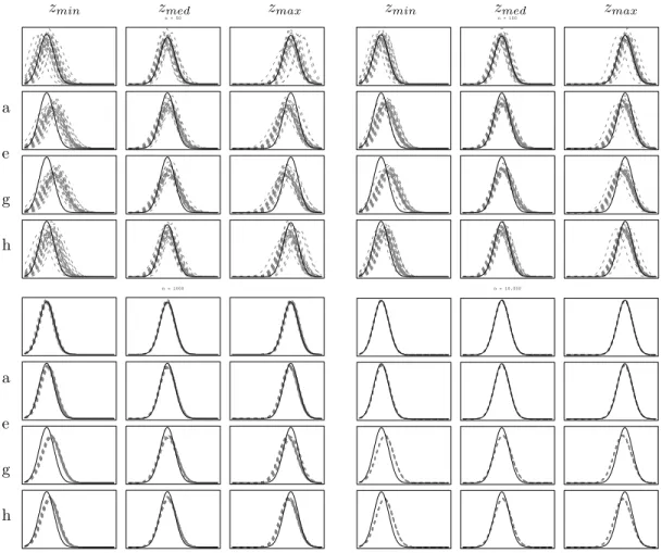
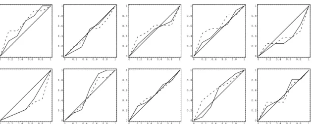
We can also investigate the calibration of the predictive and compare the entire predictive density function in (3.6) with the known sampling distribution of the response in (3.3),(3.4) or (3.5) given a particular (fixed) set of regressor variables. The fact that such predictions are, by the very nature of our regression model, conditional upon the regressors does complicate matters slightly. We cannot simply compare the sampling
to identify predictives with the value ofzf they condition on. Predicting correctly “on average” can mask arbitrarily large errors in conditional predictions, as long as they compensate each other. For Model 1, we shall graphically present comparisons of the sampling density and the predictive density for three key values
of zf within our sample of q predictors: the one leading to the smallest mean of the sampling model in
(3.3), the one leading to the median value and the one giving rise to the largest value. In addition, we
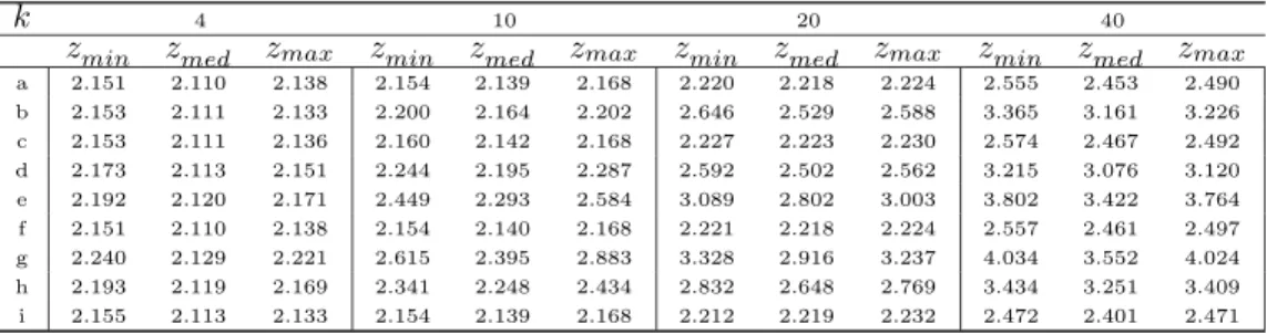
have computed quantiles of LP S and of predictive coverage over the different values ofzf as well. These
latter measures of predictive performance naturally compare each predictive with the corresponding sampling
distribution (i.e., taking the value ofzf into account), so that an overall measure can readily be computed.
4. SIMULATION RESULTS
4.1. Convergence and implementation
The implementation of the simulation study described in the previous section will be conducted through the
MC3 methodology mentioned in Section 1. This Metropolis algorithm generates a new candidate model, say
Mj, from a Uniform distribution over the subset ofMconsisting of the current state of the chain, sayMs,
and all models containing either one regressor more or one regressors less thanMs. The chain moves toMj
with probability min(1, Bjs), whereBjs is the Bayes factor in (2.16).
In order to evaluate the posterior model probabilities we can simply count the relative frequencies of model visits in the induced Markov chain. A somewhat more interesting alternative to this strategy is to use the actual Bayes factors, already computed in running the chain to compare all visited models. Since the number of visited models is typically a small subset of the total number of possible models, this method is feasible. This idea is called “window estimation” in Clyde, Desimone and Parmigiani (1996) and Lee (1996) mentions it as “Bayesian Random Search” (BARS). The generated chain is then effectively only used to indicate which models should be considered in computing Bayes factors. All other (non-visited) models will implicitly be assumed to have zero posterior probability. This has two advantages: firstly, it is clearly more precise than relative frequencies, since the Bayes factors in (2.16) are exact and don’t require any
ergodic properties. Clydeet al. (1996) provide some empirical support for this claim. Secondly, comparing
empirical relative frequencies with exact Bayes factors will give a good indication of the convergence of the chain. We shall report results based on Bayes factors, but we ran the chain for long enough to get virtually the same answers with empirical model frequencies. This was obtained with 50,000 recorded draws after a burn-in of 20,000 draws. A useful diagnostic to assess convergence of the Markov chain is the correlation coefficient of the model probabilities based on the exact Bayes factors computed through (2.16) and the relative frequencies of model visits. In our simulation experiment, this correlation coefficient was typically above 0.99. If we are interested in estimating how much of the total probability mass we have captured in the visited models, we can compare exact Bayes factors and relative frequencies of a prespecified subset of models in the way indicated in George and McCulloch (1997, Subsection 4.5).
In order to avoid results depending on the particular sample analyzed, we have generated 100 independent
samples (y, Z) according to the setup described in Section 3. Frequently, results will be presented in the
form of either means and standard deviations or quantiles computed over these 100 samples. Sample sizes
(i.e., values ofn) used in the simulation are as indicated in Subsection 3.1. Furthermore, we generateq= 19
different vectors of regressorszf for the forecasts of Models 1 and 3, whereasq= 5 for Model 2. For each of
these values of the vectorzf,v= 100 out-of-sample observations will be generated.4
Due to space limitations, we will only present the most relevant findings in detail, and will briefly sum-marize the remaining results.
4 As such a simulation study is quite CPU demanding, we put a good deal of emphasis on efficient coding and speed of
execution. We coded in standard Fortran 77, and we used stacks to store information pertaining to evaluated models in order to reduce the number of calculations. On a PowerMacintosh 7600, each 20,000–50,000 chain for Model 1 would take an average (over priors) time in seconds of: 209, 58, 15, 5, 18, and 117; forn= 50, 100, 500, 1000, 10,000 and 100,000. Since the number of visited models (and thus, the number of marginal likelihood calculations) will typically decrease withn, CPU requirements are not monotone in sample size.
4.2. Posterior model inference
4.2.1. Results under Model 1
One of the indicators of the performance of the Bayesian methodology is the posterior probability assigned to the model that has generated the data. Ideally, one would want this probability to be very high for
small or moderate values ofnthat are likely to occur in practice. Table 1 presents the means and standard
deviations across the 100 samples of (y, Z) for the posterior probability of the true model (Model 1). Columns
correspond to the six sample sizes used and rows order the different priors introduced in Subsection 3.2. In order to put these results in a better perspective, note that the prior model probability of each of the
215 possible models is equal and amounts to 3.052·10−5. We know from the theoretical results in the
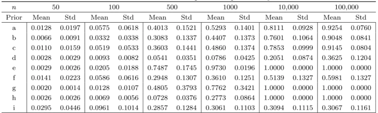
Appendix (Subsection A.1) that priors a-g are consistent. From Subsection A.2, we remain inconclusive about consistency under prior h, and we know prior i will asymptotically allocate mass to models that nest the true model. Our simulation results suggest that consistency holds for prior h (but, indeed, not for prior i) in our particular example. It is clear from Table 1 that the posterior probability of Model 1 varies greatly
in finite samples. Whereas prior e already performs very well for n = 1000, getting average probabilities
of the correct model upwards of 0.97, prior d only obtains a probability of 0.36 with a sample as large as 100,000. This result is all the more striking, since the asymptotic behaviour with both priors is the same, and they are clearly very related. This underlines the inherent sensitivity of Bayes factors to the particular
choice ofg0j. In view of this poor performance in a critical issue, we will often not give explicit results for
prior d in the sequel. Prior i does very well for small sample sizes, but then seems to taper off for values of
n≥1000 at a moderate probability for the true model around 0.3. Apart from the absolute probability of
the correct model, it is also important to examine how much posterior weight is assigned to Model 1 relative to other models. Therefore, Table 2 presents quartiles of the ratio between the posterior probability of the correct model and the highest posterior probability of any other model. It is clear that in most cases this ratio tends to be far above unity, which is reassuring as it tells us that the most favoured model will still be the correct one, even though it may not have a lot of posterior mass attached to it. For example, with
n= 50 prior g only leads to a mean posterior probability of Model 1 of 0.002 but still favours the correct
model to the next best. In fact, the correct model is always favoured in at least 75 of the 100 samples, even for small sample sizes. Note that this compares favourably to results in George and McCulloch (1993).
Table 1. Model 1: Means and Stds of the posterior probability of the true model.
n 50 100 500 1000 10,000 100,000
Prior Mean Std Mean Std Mean Std Mean Std Mean Std Mean Std
a 0.0128 0.0197 0.0575 0.0618 0.4013 0.1521 0.5293 0.1401 0.8111 0.0928 0.9254 0.0760 b 0.0066 0.0091 0.0332 0.0338 0.3083 0.1337 0.4407 0.1373 0.7601 0.1064 0.9048 0.0841 c 0.0110 0.0159 0.0519 0.0533 0.3603 0.1441 0.4860 0.1374 0.7853 0.0999 0.9145 0.0804 d 0.0028 0.0029 0.0093 0.0082 0.0541 0.0351 0.0786 0.0425 0.2051 0.0874 0.3625 0.1204 e 0.0029 0.0026 0.0205 0.0188 0.7487 0.1745 0.9730 0.0196 1.0000 0.0000 1.0000 0.0000 f 0.0141 0.0223 0.0586 0.0616 0.2948 0.1307 0.3610 0.1251 0.5139 0.1327 0.5981 0.1327 g 0.0020 0.0014 0.0128 0.0107 0.4805 0.3793 0.7762 0.3421 1.0000 0.0000 1.0000 0.0000 h 0.0026 0.0026 0.0069 0.0056 0.0728 0.0376 0.2773 0.0864 1.0000 0.0000 1.0000 0.0000 i 0.0295 0.0446 0.0961 0.1014 0.2857 0.1284 0.3061 0.1103 0.3094 0.1115 0.3067 0.1161
Table 2. Model 1: Quartiles of ratio of posterior probabilities; True Model vs Best among the rest.
n 50 100 500 1000 10,000 Prior Q1 Q2 Q3 Q1 Q2 Q3 Q1 Q2 Q3 Q1 Q2 Q3 Q1 Q2 Q3 a 1.5 3.2 6.3 3.0 5.8 8.6 3.5 13.5 20.0 9.1 19.0 29.8 27.6 67.8 90.5 b 1.1 2.6 4.2 2.2 4.1 6.2 5.5 10.8 15.3 9.6 16.6 22.1 16.6 36.3 66.3 c 1.2 3.4 5.8 2.0 5.1 8.3 7.6 13.7 18.5 7.0 13.8 22.9 26.3 55.9 73.6 e 1.6 2.7 3.5 1.9 3.8 5.8 18.8 53.6 73.6 226.5 416.4 629.4 ∞ ∞ ∞ f 1.7 4.0 7.0 2.0 4.4 8.7 5.1 10.9 14.1 4.7 9.2 16.5 9.7 19.7 24.9 g 1.4 2.3 3.3 1.4 3.9 5.1 6.3 53.9 250.2 11.4 238.7 3625.8 ∞ ∞ ∞ h 1.2 2.3 2.8 1.9 2.8 3.9 2.9 4.9 5.7 5.9 10.6 12.9 ∞ ∞ ∞ i 1.1 4.3 9.8 2.1 6.5 12.5 4.3 8.8 12.8 4.8 8.4 13.0 6.0 10.9 14.6
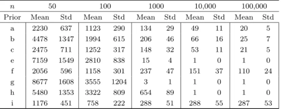
Table 3. Model 1: Means and Stds of Number of Models Visited.
n 50 100 1000 10,000 100,000
Prior Mean Std Mean Std Mean Std Mean Std Mean Std
a 2230 637 1123 290 134 29 49 11 20 5 b 4478 1347 1994 615 206 46 66 16 25 7 c 2475 711 1252 317 148 32 53 11 21 5 e 7159 1549 2810 838 15 4 1 0 1 0 f 2056 596 1158 301 237 47 151 37 110 24 g 8677 1608 3555 1204 3 1 1 0 1 0 h 5480 1353 3322 809 654 89 1 0 1 0 i 1176 451 758 222 288 51 288 55 287 53
Table 3 records means and standard deviations of the number of visited models in the 50,000 recorded
draws of the chain in model space (i.e., after the burn-in). Given that the model that generated the data is
one of the 215= 32,768 possible models examined, we would want this to be as small as possible. Forn= 50
it is clear that the sample information is rather weak, allowing the chain to wander around and visit many models: as much as around a quarter of the total amount of models for prior g, and never less than 3.5% on
average (prior i). The sampler visits fewer models asnincreases, and forn= 1000 we already have very few
visited models for prior g in particular and also for e. Of course, depending on the field of application, 1000 observations may well be considered quite a large sample. When 10,000 observations are available, that is enough to make the sampler stick to one model (the correct one) for priors e, g and h. Surprisingly, whereas
prior h still leads to very erratic behaviour of the sampler with n= 1000, it never fails to put all the mass
on the correct model for the larger sample sizes. Even with 100,000 observations, priors d and f (though consistent) still make the sampler visit 240 and 110 models on average. For prior i this is as high as 287 models.
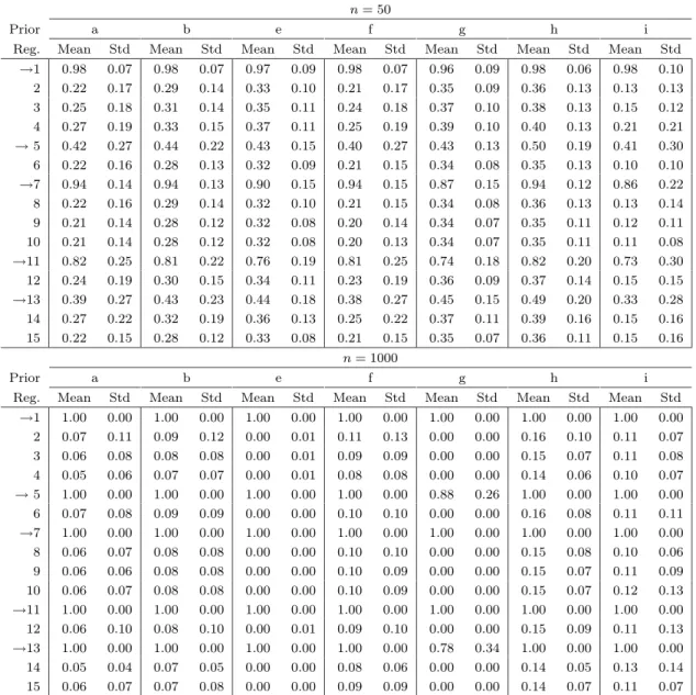
Table 4 indicates in what sense the different Bayesian models tend to err if they assign posterior probability to alternative sampling models. In particular, Table 4 presents the means and standard deviations of the posterior probabilities of including each of the regressors. As we know from (3.3), Model 1 contains regressors
1,5,7,11 and 13 (indicated with arrows in Table 4). To save space, we shall only report these results forn= 50
andn= 1000, and we will not include prior c (for which results were virtually identical to prior a) and prior
d. Whenn= 50, regressorsz(1) and z(7) are almost always included. Since they are (almost) orthogonal to
the other regressors, and their regression coefficients are rather large in absolute value, this is not surprising.
Regressorz(11)is only correlated withz(13) and is still often included. The most difficult are regressors 5 and
13, which are positively correlated, and have relatively small regression coefficients of opposite signs. The posterior probabilities of including regressors not contained in the correct model are all relatively small. Note that this is exactly where prior i excels, as the posterior probabilities of including incorrect regressors are much smaller than for the other priors. What is not clearly exemplified by Table 4 is that most priors tend to choose alternatives that are nested by Model 1 for small sample sizes, with the exception of priors d and h, which put considerable posterior mass on models that nest the correct sampling model. Table 4 informs
us that for n= 1000 the correct regressors are virtually always included. Only prior g has a tendency to
choose models that are nested by Model 1. For the other priors there remain small probabilities of incorrectly including extra regressors (the smallest for prior e and the largest for priors d and h). Alternative models tend to nest the correct model for all priors, except prior g, with this and larger sample sizes.
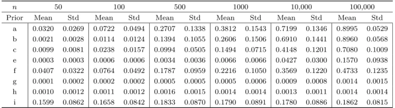
4.2.2. Results under Model 2
Let us now briefly present the results when the data are generated according to Model 2 in (3.4), the null model. Table 5 presents means and standard deviations of the posterior probability of the null model. It is
clear that this is not an easy task (see also the discussion in Freedman, 1983 and Rafteryet al., 1997) and
most priors lead to small probabilities of selecting the correct model. Overall, prior i does best for small sample sizes (followed by priors a and f), whereas larger sample sizes are most favourable to priors a and b. The behaviour of prior i is quite striking: it appears that sample size has very little influence of the posterior
probability of the correct model, making it a clear winner for values ofn≤100. Note that the other prior
where g0j does not depend on sample size, prior h, also has a posterior probability of the null model that
Table 4. Model 1: Means and Stds of Posterior Probabilities of Including each regressor.
n= 50
Prior a b e f g h i
Reg. Mean Std Mean Std Mean Std Mean Std Mean Std Mean Std Mean Std
→1 0.98 0.07 0.98 0.07 0.97 0.09 0.98 0.07 0.96 0.09 0.98 0.06 0.98 0.10 2 0.22 0.17 0.29 0.14 0.33 0.10 0.21 0.17 0.35 0.09 0.36 0.13 0.13 0.13 3 0.25 0.18 0.31 0.14 0.35 0.11 0.24 0.18 0.37 0.10 0.38 0.13 0.15 0.12 4 0.27 0.19 0.33 0.15 0.37 0.11 0.25 0.19 0.39 0.10 0.40 0.13 0.21 0.21 →5 0.42 0.27 0.44 0.22 0.43 0.15 0.40 0.27 0.43 0.13 0.50 0.19 0.41 0.30 6 0.22 0.16 0.28 0.13 0.32 0.09 0.21 0.15 0.34 0.08 0.35 0.13 0.10 0.10 →7 0.94 0.14 0.94 0.13 0.90 0.15 0.94 0.15 0.87 0.15 0.94 0.12 0.86 0.22 8 0.22 0.16 0.29 0.14 0.32 0.10 0.21 0.15 0.34 0.08 0.36 0.13 0.13 0.14 9 0.21 0.14 0.28 0.12 0.32 0.08 0.20 0.14 0.34 0.07 0.35 0.11 0.12 0.11 10 0.21 0.14 0.28 0.12 0.32 0.08 0.20 0.13 0.34 0.07 0.35 0.11 0.11 0.08 →11 0.82 0.25 0.81 0.22 0.76 0.19 0.81 0.25 0.74 0.18 0.82 0.20 0.73 0.30 12 0.24 0.19 0.30 0.15 0.34 0.11 0.23 0.19 0.36 0.09 0.37 0.14 0.15 0.15 →13 0.39 0.27 0.43 0.23 0.44 0.18 0.38 0.27 0.45 0.15 0.49 0.20 0.33 0.28 14 0.27 0.22 0.32 0.19 0.36 0.13 0.25 0.22 0.37 0.11 0.39 0.16 0.15 0.16 15 0.22 0.15 0.28 0.12 0.33 0.08 0.21 0.15 0.35 0.07 0.36 0.11 0.15 0.16 n= 1000 Prior a b e f g h i
Reg. Mean Std Mean Std Mean Std Mean Std Mean Std Mean Std Mean Std
→1 1.00 0.00 1.00 0.00 1.00 0.00 1.00 0.00 1.00 0.00 1.00 0.00 1.00 0.00 2 0.07 0.11 0.09 0.12 0.00 0.01 0.11 0.13 0.00 0.00 0.16 0.10 0.11 0.07 3 0.06 0.08 0.08 0.08 0.00 0.01 0.09 0.09 0.00 0.00 0.15 0.07 0.11 0.08 4 0.05 0.06 0.07 0.07 0.00 0.01 0.08 0.08 0.00 0.00 0.14 0.06 0.10 0.07 →5 1.00 0.00 1.00 0.00 1.00 0.00 1.00 0.00 0.88 0.26 1.00 0.00 1.00 0.00 6 0.07 0.08 0.09 0.09 0.00 0.00 0.10 0.10 0.00 0.00 0.16 0.08 0.11 0.11 →7 1.00 0.00 1.00 0.00 1.00 0.00 1.00 0.00 1.00 0.00 1.00 0.00 1.00 0.00 8 0.06 0.07 0.08 0.08 0.00 0.00 0.10 0.10 0.00 0.00 0.15 0.08 0.10 0.06 9 0.06 0.06 0.08 0.08 0.00 0.00 0.10 0.09 0.00 0.00 0.15 0.07 0.11 0.09 10 0.06 0.07 0.08 0.08 0.00 0.00 0.10 0.09 0.00 0.00 0.15 0.07 0.12 0.13 →11 1.00 0.00 1.00 0.00 1.00 0.00 1.00 0.00 1.00 0.00 1.00 0.00 1.00 0.00 12 0.06 0.10 0.08 0.10 0.00 0.01 0.09 0.10 0.00 0.00 0.15 0.09 0.11 0.13 →13 1.00 0.00 1.00 0.00 1.00 0.00 1.00 0.00 0.78 0.34 1.00 0.00 1.00 0.00 14 0.05 0.04 0.07 0.05 0.00 0.00 0.08 0.06 0.00 0.00 0.14 0.05 0.13 0.14 15 0.06 0.07 0.07 0.08 0.00 0.00 0.09 0.09 0.00 0.00 0.14 0.07 0.11 0.07
the null model, the latter is still typically favoured over the second best model. This is evidenced by Table 6, where the three quartiles of the ratio of the posterior probabilities of Model 2 and the best other model
are presented. Only prior g forn≤1000 leads to a first quartile below unity. Clearly, prior i does best for
n≤100 and prior a does best for largern. The difficulty of pinning down the correct (null) model can also
be inferred from the number of visited models (not presented in detail). Some priors (like d, e, g and h) make the chain wander a lot for small sample sizes. Priors g and h retain this problematic behaviour even
for sample sizes as large as 100,000. Interestingly, whereas prior g leads to (very slow) improvements as n
increases, the bad behaviour with prior h seems entirely unaffected by sample size, as remarked above. Of course, we know from the theory in the Appendix that priors h and i do not lead to consistent Bayes factors in this case. Whereas prior h visits on average about 12,500 models for any sample size, prior i visits around one tenth of that. The number of models visited is relatively small for priors i and a, which seem to emerge
as the clear winners from the posterior results under Model 2, respectively for small and large values ofn.
4.2.3. Results under Model 3
Now the setup of the experiment is slightly different, as we contrast various model sizes (in terms ofk) and
only two sample sizes. We would expect that the task of identifying the true model becomes harder as k
Table 5. Model 2: Means and Stds of the posterior probability of the true model.
n 50 100 500 1000 10,000 100,000
Prior Mean Std Mean Std Mean Std Mean Std Mean Std Mean Std
a 0.0320 0.0269 0.0722 0.0494 0.2707 0.1338 0.3812 0.1543 0.7199 0.1346 0.8995 0.0529 b 0.0021 0.0028 0.0114 0.0124 0.1394 0.1055 0.2606 0.1506 0.6910 0.1441 0.8960 0.0568 c 0.0099 0.0081 0.0238 0.0157 0.0994 0.0505 0.1494 0.0715 0.4148 0.1201 0.7080 0.1009 e 0.0003 0.0003 0.0006 0.0006 0.0034 0.0036 0.0066 0.0066 0.0427 0.0300 0.1570 0.0938 f 0.0407 0.0322 0.0764 0.0492 0.1787 0.0959 0.2216 0.1050 0.3569 0.1220 0.4733 0.1235 g 0.0001 0.0002 0.0002 0.0002 0.0005 0.0005 0.0005 0.0006 0.0009 0.0008 0.0014 0.0015 h 0.0010 0.0012 0.0011 0.0012 0.0016 0.0015 0.0014 0.0014 0.0013 0.0011 0.0014 0.0014 i 0.1599 0.0862 0.1658 0.0842 0.1833 0.0870 0.1790 0.0891 0.1780 0.0886 0.1862 0.0815
Table 6. Model 2: Quartiles of ratio of posterior probabilities; True Model vs Best among the rest.
n 50 100 1000 10,000 100,000 Prior Q1 Q2 Q3 Q1 Q2 Q3 Q1 Q2 Q3 Q1 Q2 Q3 Q1 Q2 Q3 a 2.4 4.4 7.0 3.1 6.2 9.2 6.0 16.1 24.8 30.0 60.0 86.2 78.7 202.4 272.1 b 2.1 5.2 7.0 3.7 6.7 9.7 7.4 22.1 28.9 18.4 45.7 79.6 64.1 153.8 253.2 c 1.3 1.8 2.1 1.2 2.2 2.7 2.0 4.1 7.1 6.3 15.2 21.8 16.1 40.3 70.2 e 1.1 2.1 2.8 1.2 2.5 3.2 2.2 3.9 5.2 3.1 6.6 9.4 6.1 11.2 16.7 f 2.4 5.3 7.5 3.5 6.8 9.3 4.9 11.4 17.5 8.1 15.7 25.3 12.9 26.9 36.2 g 0.5 1.5 2.6 0.6 1.6 2.6 0.9 2.3 3.2 1.3 2.6 3.5 1.8 3.4 4.2 h 1.2 2.3 3.2 1.3 2.5 3.2 1.3 2.7 3.2 1.7 2.7 3.5 1.6 2.5 3.1 i 4.2 8.2 13.4 5.5 10.7 13.7 4.6 9.8 14.3 6.3 10.6 14.1 4.3 9.2 14.4
(fork= 40). Of course, this may be partly offset by the fact thatσremains the same, so that the theoretical
coefficient of determination grows withk. Table 7 and 8 present the posterior probability of Model 3 in (3.5)
withn= 100 andn= 1000 observations, respectively. The first thing to notice from Table 7 is that priors
whereg0j increases withkj (priors b, e, g and h) suffer a large drop in performance as the true model (and
k) become large (k≥20 and evenk = 10 for prior g). Interestingly, prior i, which is decreasing in kdoes
not suffer from this, and performs quite well forn = 100. In fact, priors a, f and i all do remarkably well
in identifying the true model from a very large model space on the basis of a mere 100 observations. The
results fork= 40 appear less convincing, but we have to bear in mind that the posterior probability of the
correct model multiplies the corresponding prior probability by more than 1·1010 with these priors.
Table 7. Model 3: Means and Stds of the posterior probability of the true model,n= 100.
k 4 10 20 40
Prior Mean Std Mean Std Mean Std Mean Std
a 0.6993 0.1616 0.4016 0.1263 0.1745 0.0772 0.0111 0.0113 b 0.6562 0.1570 0.5970 0.1908 0.0007 0.0020 0.0000 0.0000 c 0.6408 0.1648 0.3034 0.1042 0.1116 0.0516 0.0097 0.0086 d 0.4599 0.1301 0.1589 0.0430 0.0115 0.0048 0.0000 0.0000 e 0.7269 0.1210 0.1947 0.1103 0.0000 0.0001 0.0000 0.0000 f 0.6971 0.1618 0.3986 0.1256 0.1722 0.0761 0.0107 0.0107 g 0.8036 0.1059 0.0604 0.0439 0.0000 0.0000 0.0000 0.0000 h 0.5503 0.1274 0.1676 0.0421 0.0035 0.0015 0.0000 0.0000 i 0.5084 0.1442 0.4015 0.1262 0.3145 0.1352 0.0949 0.1074
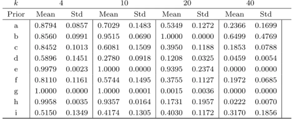
When we consider Table 8, corresponding ton= 1000, we note that most priors benefit from the larger
sample size. Only prior i leads to virtually the same posterior probabilities as with the smaller sample
(except for largek). In line with the larger sample sizen, the drop in posterior probability for the priors