Image segmentation using snakes and stochastic watershed

(1)

Image Segmentation using Snakes

and Stochastic Watershed

With Applications to Microscopy Images of Biological Tissue

Bettina Selig

Centre for Image Analysis, Uppsala

Doctoral Thesis

Swedish University of Agricultural Sciences Uppsala 2015

(2)

Acta Universitatis agriculturae Sueciae 2015:16

ISSN, 1652-6880

ISBN (print version) 978-91-576-8230-7 ISBN (electronic version) 978-91-576-8231-4

(3)

Image Segmentation using Snakes and Stochastic Watershed

Abstract

The purpose of computerized image analysis is to extract meaningful information from digital images. To be able to find interesting regions or objects in the image, first, the image needs to be segmented. This thesis concentrates on two concepts that are used for image segmentation: the snake and the stochastic watershed.

First, we focus on snakes, which are described by contours moving around on the image to find boundaries of objects. Snakes usually fail when concentric contours with similar appearance are supposed to be found successively, because it is impossible for the snake to push off one boundary and settle at the next. This thesis proposes the two-stage snake to overcome this problem. The two-stage snake introduces an intermediate snake that moves away from the influence region of the first boundary, to be able to be attracted by the second boundary. The two-stage snake approach is illustrated on fluorescence microscopy images of compression wood cross-sections for which previously no automated method existed.

Further, we discuss and evolve the idea of stochastic watershed, originally a Monte Carlo approach to determine the most salient contours in the image. This approach has room for improvement concerning runtime and suppression of falsely enhanced boundaries. In this thesis, we propose the exact evaluation of the stochastic watershed (ESW) and the robust stochastic watershed (RSW), which address these two issues separately. With the ESW, we can determine the result without any Monte Carlo simulations, but instead using graph theory. Our al-gorithm is two orders of magnitude faster than the original approach. The RSW uses noise to disrupt weak boundaries that are consistently found in larger areas. It therefore improves the results for problems where objects differ in size. To benefit from the advantages of both new methods, we merged them in the fast robust stochastic watershed (FRSW). This FRSW uses a few realizations of the ESW, adding noise as in the RSW. Finally, we illustrate the RSW and the FRSW to segment in vivo confocal microscopy images of corneal endothelium. Our meth-ods outperform the automatic segmentation algorithm in the commercial software NAVIS.

Keywords:image segmentation, snakes, active contours, stochastic watershed, min-imal spanning tree, corneal endothelium, compression wood

Author’s address:Bettina Selig, SLU, Centre for image analysis, Box 337, SE-751 05 Uppsala, Sweden

(4)

(5)

If you can dream it, you can do it.

(6)

(7)

Enclosed Publications

This thesis is based on the following papers, which are referred to in the text by their Roman numerals.

I B. Selig, C. L. Luengo Hendriks, S. Bardage and G. Borgefors, “Seg-mentation of highly lignified zones in wood fiber cross-sections”, in

Image Analysis, ser. Lecture Notes in Computer Science, A.-B. Salberg, J.Y. Hardeberg and R. Jenssen, Eds., vol. 5575, Springer Berlin Heidel-berg, pp. 369–378, 2009.

Selig developed the methods, designed and performed the experiments, and wrote the paper.

II B. Selig, C. L. Luengo Hendriks, S. Bardage, G. Daniel and G. Borge-fors, “Automatic measurement of compression wood cell attributes in fluorescence microscopy images”,Journal of Microscopy, vol. 246, no. 3, pp. 298–308, 2012.

III B. Selig and C. L. Luengo Hendriks, “Stochastic watershed—an ana-lysis”, inProceedings of SSBA 2012, Swedish Society for Automated Im-age Analysis, pp. 82–85, 2012.

Selig designed and performed the experiments, and wrote the paper. IV F. Malmberg, B. Selig and C. Luengo Hendriks, “Exact evaluation of

stochastic watersheds: from trees to general graphs”, in Discrete Geo-metry for Computer Imagery, ser. Lecture Notes in Computer Science, E. Barcucci, A. Frosini and S. Rinaldi, Eds., vol. 8668, Springer Inter-national Publishing, pp. 309–319, 2014.

Selig wrote a great part of the program, performed the experiments and co-authored the paper.

V K. B. Bernander, K. Gustavsson, B. Selig, I.-M. Sintorn and C. L. Lu-engo Hendriks, “Improving the stochastic watershed”, Pattern Recog-nition Letters, vol. 34, no. 9, pp. 993–1000, 2013.

Selig developed the methods, designed the experiments and co-authored the paper.

VI B. Selig, F. Malmberg and C. L. Luengo Hendriks, “The fast evalution of the robust stochstic watershed”, submitted for publication in a con-ference proceeding, 2015.

(8)

VII B. Selig, K. A. Vermeer, B. Rieger, T. Hillenaar and C. L. Luengo Hendriks, “Fully automatic evaluation of the corneal endothelium from in vivo confocal microscopy”, submitted for journal publication, 2015. Selig developed the methods, designed and performed the experiments, and wrote the first draft of the paper.

Reprints were made with permission from the publishers.

Related work

While working on this thesis, the author also contributed to the following papers

viii B. Selig, C. L. Luengo Hendriks and G. Borgefors, “Measuring distribu-tion of lignin in wood fibre cross-secdistribu-tions”, inProceedings of SSBA 2009, Swedish Society for Automated Image Analysis, pp. 5–8, 2009.

ix B. Selig, M. K. Khan and I. Nyström, “Using a ring-shaped region around the optic disc in retinal image registration of glaucoma patients”, in Pro-ceedings of SSBA 2010, Swedish Society for Automated Image Analysis, pp. 35–38, 2010.

(9)

1 Introduction

1.1 Image segmentation

The key task in image analysis is to extract meaningful information from a digital image. The area of application is diverse. Image analysis can be used for example to classify soil in remote sensing images[26], to recognize faces[50]using security systems or to detect tumors in medical images[4] to diagnose and plan possible treatment.

To extract information from an image, interesting regions or objects need to be found. For this, the image needs to be partitioned in coherent regions. This procedure is calledsegmentation, and the result is a segmented image, in which each pixel is assigned a label representing an object or the background. Finally, we can obtain information for the labeled regions in form of measurements.

Often correct segmentation is the most difficult task for image analysis applications. A prerequisite for an automatic segmentation algorithm is that it is possible to distinguish between different objects. This is provided when the objects differ, for example, in color, size or texture. Since the input data for the different applications differs strongly from each other, a universal segmentation method cannot be provided. Instead, we have to tailor a suitable procedure to every new problem. For this, a multitude of segmentation algorithms exist which all serve different purposes and are useful for different problems.

If the objects hold different colors, that is intensities in grey value im-ages, various methods, as thresholding [36]or k-means [23], can be ap-plied. If the extent is known to which pixels belonging to the same region differ from each other, region growing methods like statistical region mer-ging[31]are useful.

Often it is beneficial to regard thegradient magnitude, which is the dif-ference in grey value of neighboring pixels: where the gradient magnitude is low, neighboring pixels have similar grey values and probably belong to the same object, and where the gradient magnitude is high, the grey value of neighboring pixels differs strongly. In the latter case, an edge in the image is present, which potentially belongs to the contour of an object.

There are many different ways to use the gradient to find the desired outline, for example Canny’s edge detector[9]or graph-based methods like Markov Random Fields[43].

In this thesis, we focus on the two segmentation approachessnakes[24]

andstochastic watersheds[1].

(12)

ap-proximate location of its contour are known, for example organs in medical images[20]. Snakes are active contour models, which attempt to minimize an energy functional that is based on attributes of the image and the expec-ted shape of the object’s contour. For this, the snake is defined as aspline, a piecewise polynomial function described by a set of points. It is moved over the image to settle at the position of an energy minimum, which is ideally the object’s contour.

The stochastic watershed approach is suitable for the segmentation of structures composed of similarly sized regions and where an approximate number of objects is known, for example multispectral satellite images[33]. The algorithm determines the most salient boundaries in the image using

Monte Carlo simulations, which means repeated random sampling. Sali-ent boundaries are expected to occur more frequSali-ently during the attempts, which are used to determine a final segmentation.

1.2 Thesis outline

Section 2 describes the basic approach of active contour models and pro-poses the two-stage snake, a variant to find similar boundaries successively.

Section 3 explains the stochastic watershed approach and proposes sev-eral versions of the method to overcome two problems, such as high com-putational costs and falsely enhanced boundaries. Finally, the new methods are compared to each other and to the original approach.

Section 4 shows an application with fluorescence microscopy images of compression wood cross-sections. The appearance of the fibers consists of concentric regions. To segment these regions, we apply the two-stage snake. Afterwards, we compare the segmentation to the delineation done by two experts.

Section 5 concentrates on the segmentation and measurement of in vivo confocal images of human corneal endothelium. We apply two of our pro-posed stochastic watershed approaches and show that we achieve more ac-curate results than the commercial software NAVIS.

(13)

2 Segmentation using snakes

2.1 Basic approach

Active contours are methods to delineate the boundaries of objects in an image. These approaches are especially useful when parts of the desired boundaries are missing or otherwise difficult to detect.

The two main active contour methods are level sets[35]and snakes[24]. The level set approach is based on the level set function, which is modified by applied forces. The zero level set, the set of points where the function crosses the xy-plane, is the outline of the desired object(s). This approach has the feature that contours can split and merge during the process. It is often used to track moving objects[37].

A snake is implemented as the splinev(s) = [x(s),y(s)], wherex(s)and

y(s)are thexy-coordinates along the contours∈[0, 1]. Often the snake is

described as a closed contour, since it ought to find the outline of an object. This means v(0) =v(1), the position of the start and the end point of the

snake are the same.

The snake approach is suitable if the appearance and the approximate location of the desired contour are known. Snakes are less complex and easier to implement than level sets. Since in the application presented in Papers I and II it is not necessary to split or merge contours, we were able to use the simpler snake approach.

After initializing the snake as close as possible to the expected location of the targeted contour, the snake is moved around to gradually minimize the energy functionalE_snake, defined as

E_snake=E_int+E_ext, (1) whereE_intis an internal energy that defines the favored shape of the snake, for example short and straight, andE_extis an external energy that is based on the attributes of the image and enables the snake to find the outline of the desired object.

The internal energyE_intis defined as

E_int=α|dv ds| 2₊_β|d 2_v ds2| 2_, ₍₂₎

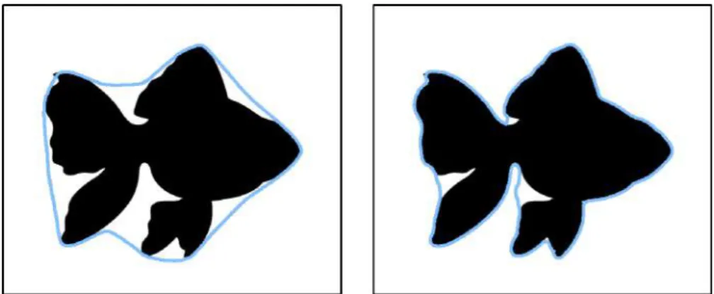
where the parametersαandβregulate elasticity and stiffness, respectively. When increasingα, the first term gains relevance. This means that the snake prefers to be short, acts more like a rubber band around an object and does not necessary delineate concave areas well. When increasingβ, the second

(14)

Figure 1: Example for snakes whenα=1 andβ=0 (left), and whenα=0 andβ=1 (right).

term gains relevance, which makes the snake smooth and avoids the forma-tion of sharp edges, see Fig. 1.

The external energy is traditionally based on the gradient magnitude of the imageI(x,y), as

E_ext=−|∇I(x,y)|2. (3) This makes the snake settle in regions with high gradient, that is boundaries. The forces that are applied to the snake during the minimization process are the derivatives of the present energies:

~ F_int=− ∇Eint ||∇E_int|| (4) and ~ F_ext=− ∇Eext ||∇E_ext||. (5)

The gradient vector flow (GVF)[49]produces an alternative external force that is more suitable if the snake is initialized far away of the desired contour or the contour has concave sections. A GVF field is created that applies a constant (normalized) force on each point of the image. To de-termine the GVF field, we need to find the force F~_GVF = (U_GVF,V_GVF)T

that minimizes the energy functional

E_GVF=

Z

µ(|∇U_GVF|2+|∇V_GVF|2)+|∇E_ext|2|~F_GVF+∇E_ext|dx, (6) whereµis to balance the influence of the green and blue terms. The blue term in the energy functionalE_GVFensures that the direction of the force is

(15)

equal to the direction of the earlier defined external forceF~_extin regions of high gradient, which means close to edges. In regions of low gradient,F~_ext

contains too little information and is not able to push the snake towards desired contours. The green term in the function for E_GVF makes these regions smooth, which means that the information of the boundaries of the regions is spread over the whole region. The result is that boundaries have a larger influence region and the snake will be attracted to them even when it is initialized far away. Additionally, the snake improves delineating the contour of an object, if it has a concave outline.

If only the internal force is applied to the snake and the snake is ini-tialized inside the object, the contour of the model shrinks and finally col-lapses. To make sure that the snake is pushed outwards to reach the desired boundary, an additional force, called balloon force, is often used. A small force is applied orthogonal to the outline of the snake. It is added to F~_ext, alternatively toF~_GVF, as

~

F_ext₊_balloon=c~Fext+cp~n(s). (7) The parametercis the weighting of the external force andcpis the weight-ing of the balloon force.

Since the snake approach builds on energy minimization using gradient descent, there might not be an optimal final position for the snake and after a while the snake might oscillate between two locations. One can define an

εthat determines a minimal energy left in the system or a maximal distance moved within the last steps. But this parameter is not always easy to define and when the snake overshoots the desired boundary and does not settle at all, it is anyway necessary to have a maximal number of iterations. There-fore, sometimes it is easier to have only a maximal number of iterations as stopping criterion.

2.2 Two-stage snakes

When using snakes to successively find boundaries of concentric regions, we face a problem. If the desired boundaries have similar conditions, for example, are transitions from darker to lighter regions, it is impossible for the snake to push off the first boundary and then settle at the second. This is because the same forces that make the snake move away from the first boundary, prohibits stopping the ongoing movement at the second bound-ary and instead pushes the snake further away.

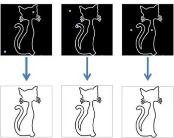
To overcome this problem, we introduced an intermediate step in Pa-per I: after the snake traced the outline of the first boundary, we apply a

(16)

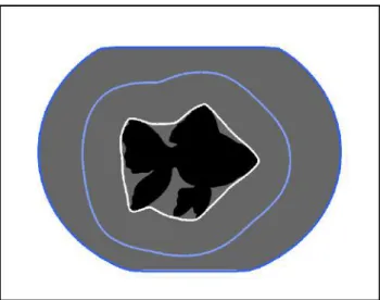
Figure 2: Illustration of two-stage snake: Initialization (white line), inter-mediate steps (light blue line) and final segmentation (dark blue line). new external force to the snake (with an additional balloon force). We call this new forcecomplementary force. The corresponding energy describes a minimum between the two desired boundaries, as for example−F_ext.

The result of applying the complementary force is that the snake moves outwards (due to the balloon force) to settle at a position between the two desired boundaries. From this new position, the initial external force can be applied again, so the snake is attracted by the second, the outer boundary, see Fig. 2. This approach has the advantage that no additional parameters are needed. Only the complementary force needs to be determined.

A prerequisite for this new force is that the complementary energy has its minimum between the desired contours. Otherwise the snake passes the contour during the intermediate step and then cannot retract in the final step, due to the added balloon force.

(17)

3 Segmentation using stochastic watershed

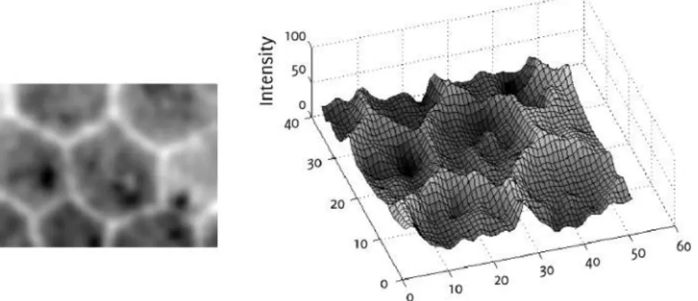
Figure 3: Endothelial cell image (left) and representation as geodesic land-scape (right).

3.1 Basic watershed methods

In thewatershed segmentationalgorithms[6], we regard the image as a geo-desic landscape. Low gray level values correspond to valleys and high val-ues to hills, see Fig. 3. When the water level raises, each local minimum functions as water source, since water emerges from it. The landscape is subsequently flooded. Eventually, the water of two minima meet at the ridgeline between their catchment basins, where now a watershed line is placed. Hence, the watershed segmentation separates regions that yield pre-cisely one minimum.

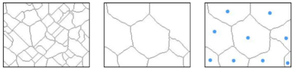
Digital images, as e.g. microscopy images, usually suffer from noise, so that the desired region often contains more than one local minimum. Therefore, the basic watershed approach often yields an over-segmented res-ult, see Fig. 4.

To reduce the number of segmented regions, we can use theH-minima transform, see Fig. 4. Here, all minima that have a depth less thanhare sup-pressed and therefore are not used as sources during the immersion process. The idea to remove the most shallow minima is based on the assumption that these minima are least important. But due to non-uniform lighting conditions or different amounts of contrast in the image, this method alone is sometimes not sufficient to give satisfactory segmentation results.

In case the rough positions of the desired regions are known,seeded wa-tershed can be used, see Fig. 4. First, we set a seed point for each region

(18)

Figure 4: Segmentation results of example image in Fig. 3 using different watershed approaches: watershed segmentation (left), watershed segmenta-tion using H-minima (middle), seeded watershed segmentasegmenta-tion (right). Dots show the locations of the seed points.

manually or automatically. These seed points then function as sources for the flooding operation described above, whereas the local minima are ig-nored. However, positioning the seed points is not a trivial task. Using a manual approach is not feasible for many applications, because it is too time consuming. And finding the regions automatically transforms the segment-ation task into a problem of object detection.

Later, we concentrate on more elaborate watershed methods, but first, we explain how a basic watershed segmentation can be obtained.

3.2 Concepts to determine a watershed segmentation

There are several algorithms to obtain a watershed segmentation of a given image. In this section, we first regard two attempts that simulate the idea of flooding a landscape, and later discuss the possibility of transferring the problem to graph theory.

The concept of raising the water level of the image (immersion simula-tion), is mimicked by an algorithm published by Vincent and Soille [46]. Here, we describe a variation of this method.

First, we sort all pixels in the image according to their gray level. Then, we regard the pixelv with the smallest value and remove it from the sorted list. To determine if v belongs to one region or to a watershed line, we regard the following three cases: 1) If none ofv’s neighbors is labeled, create a new label forv. 2) If there exists only one label in the neighborhood, we label v with that label. 3) If the neighborhood contains more labels, we markv as watershed pixel. We proceed with the algorithm by continuing processing the pixels in the sorted list, until the list is empty and all pixels are either labeled or marked as watershed pixels.

Another more common approach is the flooding simulation introduced by Beucher and Meyer[7]. It is based on the idea that the water emits from

(19)

water sources, which are either all local minima in the image (standard wa-tershed) or a set of chosen seed points (seeded wawa-tershed). For simplifica-tions, we call these water sourcesmarkers.

As a first step, we label all markers individually. Next, we add all neigh-boring pixels of the initial markers in a priority queue, where the priority is the gray level value of the pixel. Now we visit and extract the pixelvwith the highest priority (lowest gray value) from the queue. If all labeled neigh-bors ofvhave the same label,vis also labeled with their label. If the labeled neighbors have different labels,v is marked as a watershed pixel. Pixels of the neighborhood that have not been visited yet are now inserted in the pri-ority queue. We continue to process the pixels in the pripri-ority queue until the queue is empty and all pixels in the image are visited.

A digital image can be transferred to a edge-weighted graphG, where vertices V correspond to the pixels in the image and the weights of the edgesEto the similarity of the pixels, e.g. the difference in grey values. In this representation, the watershed segmentation can be solved bywatershed cuts, introduced by Cousty et. al[13].

Where the watershed in an image is defined by pixels that form the boundaries between the regions, a watershed cut is a set S_G of edges that, when removed, splits the graphGinto two or more disjoint connected com-ponents (representing the found regions).

To simplify the problem, we only regard the minimal spanning tree

(MST) T. The MST is a subgraph ofG that connects all verticesV and in addition, has a minimal total edge weight.

The result of the watershed cut algorithm is aminimal spanning forest

(MSF)GF of the original graph, where each connected component contains exactly one marker. This MSF is not only a subgraph ofG, but also a sub-graph ofT. Since the regions of the watershed segmentation are defined by markers, the watershed cutSG of the complete graph corresponds to water-shed cutS_T of the MST. The MSFG_F can be computed by any algorithm creating an MSTT with some additional conditions[28].

There are two basic algorithms that are often used to create the MST of a graph. They were introduced by Kruskal[25]and Prim[39], respect-ively. When inspecting the procedure of these two algorithms, one finds correlations to the two concepts of computing a watershed segmentation, described above. Kruskal’s approach functions similar to the immersion principle and Prim’s algorithm to the flooding simulation method.

When producing the MSF instead of the MST, we need to alter the ori-ginal algorithms slightly: to ensure that each connected component con-tains exactly one marker, we do not include edges of the MST that establish

(20)

a path between markers in the resulting graph.

When creating an MSF using an algorithm based on Kruskal’s idea, we proceed as follows: first, we set all vertices as unlabeled and sort all edges according to their weights. Next, we regard the edgee_vw with the smallest weight (connectingv andw) and remove it from the sorted list. To determ-ine if e_vw belongs to the MSF, we consider the following three cases: 1) If both verticesvandware not labeled, create one new label for both vertices and includee_vw to the MSF. 2) If only one vertex is labeled, label the other vertex with the same label and includee_vw to the MSF. 3) If both vertices

v and w are labeled, do not include e_vw in the MSF. Including this edge would either form a cycle in the graph or connect components with dif-ferent local minima. Afterwards, continue proceeding with the next edge from the sorted list until all edges have been processed and the list is empty. Contrary to Kruskal’s method, with Prim’s algorithm we can set mark-ers from where the regions expand. To create an MSF with a Prim-like approach, we first label all markers with an individual label. Next, we add all edges adjacent to the markers in a priority queue, where the priority is the weight of the edges. Then, we visit and extract the edgee_vw with the highest priority (lowest weight) from the queue. If only one vertex,v orw, is labeled, we label the other vertex with the same label and includee_vw to the MSF. We also enqueue the edges connected to the newly labeled vertex in the priority queue. But if both v andw are already labeled, we do not includee_vwin the MSF. Including this edge would either form a cycle to the graph or connect components that contain a marker each. Now, we proceed with the next edge from the priority queue until all edges have been visited and the queue is empty.

The labeled components in both methods now represent the segmented regions. To create a watershed line between the regions in the image repres-entation, we can, for example, mark pixels that are neighbors to pixels with a different label as watershed pixels. As a result, the watershed lines are two pixels thick.

3.3 Stochastic watershed

The ideal segmentation algorithm produces a perfect segmentation result without the user providing any previous knowledge. Unfortunately, this is not a realistic vision, since it has to be defined how the important object(s) can be distinguished from the rest of the image.

More realistic is to develop an algorithm with a small number of para-meters, which also are intuitive to select. The stochastic watershed, which was proposed by Angulo and Jeulin[1], is moving in this direction.

(21)

Figure 5: Gradient magnitude with seed points placed in different regions (top) and segmentation results (bottom).

This algorithm has three parameters: the number of seed pointsN, the number of realizations M and the number of most significant regions R. The number of seed points N and the number of most significant regions

Rare directly related to the number of objects that ought to be segmented. The number of realizationsM defines how precise the segmentation result is in relation to the time spent on the calculations.

The stochastic watershed utilizes a property of the seeded watershed, which is that the algorithm is very insensitive to the placement of seed points within a region: Considering two neighboring regions, their seed points can move large distances in each respective region and the result still yields the same segmentation line. This is due to the order in which the pixels are processed, see Fig. 5.

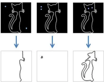
The stochastic watershed uses Monte Carlo simulations to find salient boundaries. Here, seeded watershed with randomly placed seed points is ap-plied repeatedly to the image. Whether the boundary between two neigh-boring regions will be detected depends on the random placement of the seed points in these regions. There are two cases: 1) Each of the regions contain (at least) one seed point, or 2) only one or none of the regions con-tain seed points.

In the first case, the boundary between the regions is found, due to the property of the seeded watershed, described above. In the second case, the boundary between the two regions will normally not be found at all or only found as fragments, see Fig. 6. (Sometimes, when seed points in other parts

(22)

Figure 6: Gradient magnitude with seed points placed in the same region (top) and segmentation results (bottom).

of the image are placed advantageously, the boundary can be found anyway, but for now, we refrain from these cases.)

The probability is high that salient boundaries are found when applying seeded watershed with randomly placed seed points. When this step is pro-ceeded repeatedly, a probability density function (PDF) of the boundaries can be determined.

In order to obtain a segmentation using stochastic watershed, Angulo and Jeulin[1]createM realizations of seeded watershed withN randomly placed seed points. They then construct the PDF combining the M seg-mentations using the Parzen window method. In our versions of the al-gorithm, we simply add the segmentation results to create the PDF.

Finally, Angulo and Jeulin segment the PDF with volumic watershed for defining theRmost significant regions. This last step of segmenting the PDF into R regions, we changed in our versions to a standard watershed segmentation with H-minima transform, where all minima are erased that are smaller than a threshold h. This seems to be more fitting to many ap-plications, because we do not persist in having exactlyRregions in the final segmentation. Especially when the image contains a multitude of objects, the user is often only able to provide a rough estimate for the number of desired objects. Even though the parameterhin the H-minima transform is barely intuitive to choose, this approach often yields a better segmentation result. As described before, the H-minima assumes that the most shallow minima are the least important. Since we are operating on an image

(23)

repres-enting the significance of boundaries in the image, this assumption is true and therefore the H-minima transform is suitable to apply.

In the remainder of this thesis, when we refer to the stochastic water-shed segmentation algorithm, we mean a version of the original method where we determine the PDF by simply adding the M seeded watershed segmentations and create the final result using the standard watershed with H-minima transform.

3.4 Parameters

In Paper III, we focused on the first part of the stochastic watershed, where the PDF is created, and studied the relation between the algorithm’s para-meterN and the actual number of regions in the image. We discovered that the value ofN has a great influence of how many realizations of the seeded watershed are needed to make a good segmentation of the PDF possible.

To show this, we created three synthetic images with different num-bers of equally sized regions. With these images and different values forN, we determined the minimal number of realizations M_min to create a PDF, where the original boundaries can be distinguished from the background through thresholding. From the results, we concluded that the algorithm is not very sensitive to the value ofN, but that when choosing N close to the actual number of regions in the image,M_minis lowest. This means that the distinction between boundaries and background is possible with fewer realizations.

The disparity of boundary and background values in the PDF grows over time (according to our experiments). Hence, the smaller M_minis, the easier it is to achieve a good segmentation of the final PDF (afterM realiza-tions).

Even though we noted that the stochastic watershed is not very sensitive to the value ofN, it cannot be set arbitrarily, but needs to be chosen for the application by visual inspection or training. IfN is set too small, small de-tails in the image can be lost, and by choosing it too large, weak boundaries could be found repeatedly, which results in an over-segmentation.

The parametersMandhare dependent on how difficult it is to segment the desired objects in the image. If it is simple to detect the boundaries, a suitable segmentation can be determined after only a few realizations of the seeded watershed. Additionally, the algorithm is not that sensitive to the threshold h, due to the disparity of boundary and background values in the PDF mentioned before. However, if the boundaries are unclear, we need more realizations to determine a reliable result. Because of this, the value for M is often set to 50 or 100[16, 34]. Additionally, the algorithm

(24)

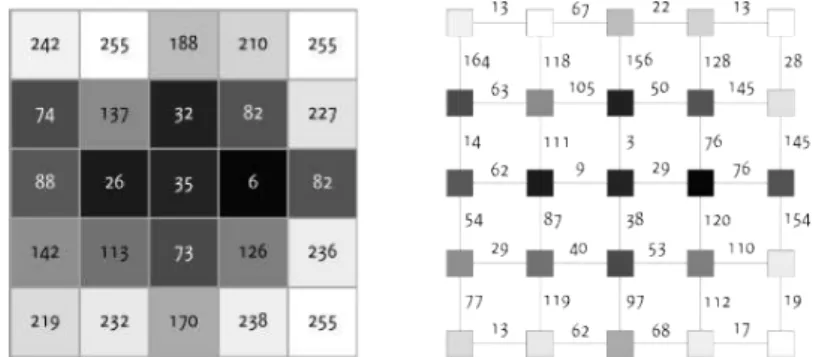
Figure 7: Original image (left) and edge-weighted graphG(right). The value of the edge weights is the absolute difference of the gray value of the neigh-boring pixels connected by the edge.

Figure 8: MSTT (left) and forestG0(right). To constructG0all edges with weights greater or equal to the weight ofe_ABare removed fromT. The trees

TAandTB are presented in red and blue, respectively.

gets more sensitive toh, because real boundaries and falsely enhanced lines might not be separable in the PDF.

3.5 Exact evaluation of the stochastic watershed

Due to the multiple realizations of seeded watershed that are needed to ob-tain a useful estimate of the PDF, the SW is not very fast. For this, Meyer and Stawiaski[29]worked on a way to determine the PDF exactly, without Monte Carlo simulations. Malmberg and Luengo Hendriks[27]extended this approach and presented an efficient algorithm to calculate the exact PDF.

Meyer and Stawiaski[29]developed a formula to calculate the probab-ility that neighboring pixels are in different regions, when using randomly

(25)

placed seed points. For this, we regard the MST T of the edge-weighted graphGrepresentation of the input image, see Fig. 7.

We explain the concept by determining the probability that the vertices

AandB in Fig. 8 are in different regions. That means that edgee_AB connect-ingAandB is included in a watershed cutST. In our example, the edgeeAB has the value 40. Since all edges greater or equal to this value are not relev-ant for this case, we remove all these edges fromT. The result is a forestG0, in which one of the trees contains vertexAand another one contains vertex

B. These trees we callT_AandT_B, respectively, see Fig. 8.

The probability thatAandB lie in different regions corresponds to the probability that seed points fall in both the area presented by T_A andT_B. To compute this probability, we consider thatρ(v)is the probability that the pixel represented by vertexv is a seed point. If all pixels have the same probability to be chosen as a seed point, thenρ(v) =_|V1_|, whereV is the set of all vertices.

Hence, the probability that a seed point is placed within a subtreeT0is

f

T0= X v∈V(T0)

ρ(v). (8)

This means that the probability that Aand B lie in different regions, when usingN randomly placed seed points, is

F(fT_A,Tf_B) =1−(1−Tf_A)N−(1−Tf_B)N+(1−Tf_A−Tf_B)N, (9)

where the blue and red terms specify the probability that there is no seed point inT_AorT_B, respectively, and the green term describes the probability that in neither of the trees T_A orT_B there is a seed point. The green term needs to be added as an adjustment, since we considered the case that there is no seed point in both trees, T_A and T_B, twice (in the blue and the red term).

Malmberg and Luengo Hendriks[27]developed an efficient, quasi-linear algorithm to enable this approach. The efficiency of this method lies in the usage of disjoint-set data structures. These data structures keep track of connected components formed when edges are added to a graph.

The proposed algorithm works as follows: after transforming the image into a edge-weighted graphG and determining the MSTT, all edges ofT

are sorted and stored in a listC. First, the edgee_ABwith the minimal weight (connecting the verticesAandB) is regarded. To set a probability value for this edge to be included in a watershed cut S_T, we consider the subgraph

(26)

Figure 9: TreeTPDF(weights not shown).

regard the connected components (trees)T_AandT_B. Now, we can calculate the probability F(fT_A,Tf_B) that e_AB is in a watershed cut S_T. Finally, we

extracte_AB fromC and continue with the next smallest edge inC untilC

is empty and all edges are processed.

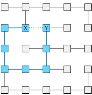
The result of this algorithm is a treeT_PDF with probability values as edge weights. This representation of the PDF is difficult to visualize. For further processing, it can be useful to transform the tree to a PDF image. In Paper IV, we propose a method to extend the tree representation of the PDF to a graphG_PDFthat can be further processed to an image.

We illustrate our approach on the treeT_PDFshown in Fig. 9. For this, we consider the edgee_{X Y}, which connects the verticesX andY inG_PDF, but is not present inT_PDF. Further, we regard the pathπ_{X Y} (blue in Fig. 9) connectingX andY inT_PDF.

IfX and Y are in different regions, at least one edge alongπ_{X Y} must have been cut. Therefore, the probability that e_{X Y} is included in a water-shed cut S_G_PDF, corresponds to the probability that at least one edge along

πX Y is included in the watershed cutST_PDF. Therefore, the probability is defined as

P(e_{X Y}) =1− Y

e∈E(πX Y)

(1−P(e)). (10)

In Paper IV, we propose an efficient algorithm that calculates this prob-ability for all edges in the graphGin linear time. For this, we first define a function

φ(X,Y) =1−P(e_{X Y}) = Y e∈E(πX Y)

(1−P(e)). (11) Additionally, we choose an arbitrary vertex inT_PDFto be the root R. We defineφ_R(v) =φ(v,R)for any vertexvin the tree.

(27)

We now can calculate the probability ofe_{X Y} being included in a water-shed cutSG by

φ(X,Y) = φR(X)φR(Y)

(φR(LCA(X,Y)))2

, (12)

where LCA(X,Y)is thelowest common ancestor of the two verticesX and

Y. An ancestor of a vertexv is a vertex that lies on the direct path toR. Further, a lowest common ancestor of verticesv andw is ancestor tov as well as towand lies farthest away fromR.

In our algorithm, we first calculateφ_R(v) by traversing all verticesv

via breadth-first search. Afterwards, we calculate P(e_vw) for all edges in

G_PDF. For this, we need to determine LCA(v,w). Using the algorithm by

Bender and Farach-Colton[5], this step can be done in constant time, after an O(|V|)preprocessing step. This concept is based on an idea by Harel and Tarjan[21]and is mainly responsible for the efficiency of the ESW.

To finally transformG_PDFto an image, we need to determine for each pixelv how probable it is that a pixelwin the neighborhoodδ(v)lies in a different region. This corresponds to the probability that at least one of the edges connected tov is included in a watershed cutS_G, which is defined as

PG(v) =1−

Y

w∈δ(v)

(1−P(evw)). (13)

3.6 Robust stochastic watershed

In Paper III, we first observed that the stochastic watershed works best when the regions in the image are similarly sized. Since the probability of placing a seed point is the same over the image, large areas often receive several seed points and small regions possibly none. This means that the algorithm tends to split large area and miss small ones.

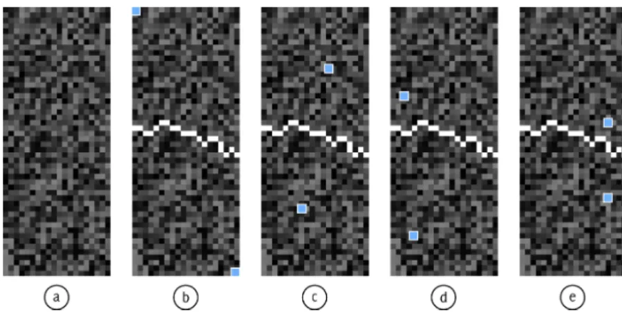
To understand the origin of falsely enhanced lines, we regard the case that one region contains two seed points. In Fig. 10(b), the seed points are placed as far from each other as possible. To find the boundary between the two regions specified by the seed points, neighboring pixels to the emerging regions will be successively assigned to one of the seed points. The order in which the pixels are assigned is defined by their gray values, as described be-fore. This specific order does not change when we position the seed points elsewhere in their respective regions, see other examples in Fig. 10(c-e). This means that the algorithm will always find the same boundary as long as there is one or several seed points present in each of the regions. This hap-pens regardless of whether there was an actual boundary located in the

(28)

ori-Figure 10: Examples to illustrate that a boundary does not change when changing positions of seed points.

ginal image or if the algorithm falsely enhances a non-existing boundary and thus fabricates a so calledfalse boundary.

The insensitivity to the placement of the seed points usually enables the stochastic watershed segmentation to find reliably relevant boundaries, but, in the case of false boundaries, it works to our disadvantage.

To handle this issue, we introduced two improvements presented in Pa-per V. Firstly, we add noise to the image before each realization of seeded watershed, and secondly, we place the seed points in a grid with random offset and rotation.

The reason for the occurrence of false boundaries is that each realization uses the exact same order in which the pixels are assigned to regions. One way to alter the order in which the pixels are processed, is to add a small amount of noise to the original image before each realization. This does not affect the image boundaries, but mixes up the local rank order. In our experiments, we received best results with noise stronger than the noise in the input image, but not strong enough to hide the signal.

In Paper V, we noted that the amount of noise can be determened with the help of a noise estimation of the image, e.g. using the method by Im-merkaer [22]. However, in later experiments (not reported), we did not find any correlation between the optimal amount of noise and the estim-ated noise strength in the input image.

The idea behind the second improvement, placing the seed points on a grid, is the following: when seed points are placed directly next to each other (as it happens using the Poisson process), a segmentation line is forced to be set between them. The idea of placing them in a grid, is to increase

(29)

their distance to each other as much as possible, so the influence of the image values on the segmentation is maximized and the dependency of the seed point positions is minimized.

However, our experiments showed that the grid (square or hexagonal) only improved the segmentation in combination with the first modific-ation. Without adding noise to each realization, the formation of false boundaries dominated the PDF in such a way that the benefit was not ap-parent.

Just as in the SW, the optimal number of seed points in the RSW lies around the actual number of regions in the image. Using fewer seed points has similar effects on both methods: the number of realizations needed in-creases. When increasing the number of seed points, the SW breaks down, since at some point false boundaries dominate the PDF. In contrast, the RSW was less affected by the number of seed points and still produced use-ful PDFs using four times the optimal number of seed points. We concluded that the RSW is less sensitive to the choice ofN compared to the SW. By the way, the sensitivity of the RSW to the parameters M and h did not differ from the SW.

3.7 Fast evaluation of the robust stochastic watershed

With the RSW, we overcome a major drawback, namely the tendency of the SW to segment the image into similarly sized regions. But since the RSW also uses the idea of Monte Carlo simulations, the runtime is similar to the SW. With the ESW, we could speed up the SW algorithm, but this method does not seem easily compatible with the RSW.

While the RSW requires several realizations of the seeded watershed, the ESW works on a graph representation, more precisely the MST, of the image. To imitate the idea of adding noise to the original image, like in the RSW, we would need to combine several trees in one graph. This is not a trivial task. In Paper VI, we developed a hybrid approach instead and called it thefast evaluation of the robust stochastic watershed(FRSW).

Using the ESW approach, seed point placement is no longer an issue, so we ignore the advantage of placing the seed points in a grid. Further, we abandoned the idea of incorporating the addition of noise in the ESW, and instead perform the ESW several times by using the original image with a small amount of noise added.

The RSW typically uses about 50-100 realizations of seeded watershed. This number of realizations M is chosen to match the conditions of the SW. The ESW determines the result forM =∞within one step. Since we use the ESW repeatedly in our approach published in Paper VI, the

(30)

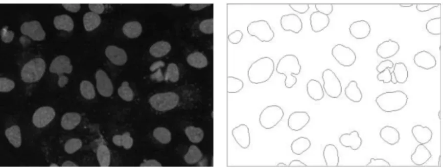
num-Figure 11: Example image of data set (left) and its hand-drawn ground truth (right).

ber of realizations M_f can be much smaller and still produce good results. The value ofM_f is only related to the required number of noise images to suppress false boundaries.

To get the most information out of theM_f intermediate PDFs as pos-sible, we merge them in an advantageous way to obtain the final PDF. In Paper VI, we found the geometric mean a suitable method, since lines (even though they might be weak) present in most PDFs are preserved and lines present in only a minority of the PDFs are suppressed. The geometric mean of the pixelx_iat positioni in the final PDF is determined as

xi= Mf Y m=1 xi,m ! 1 M f , (14)

wherex_i_,_mis the pixel at positioniin them-th intermediate PDF.

In our experiments, we showed that the FRSW achieves segmentation results on par with the RSW, when usingM_f =3 (compared to RSW using

M=50). Since the complexity of the calculation of one realization of ESW is similar to one realization of seeded watershed, the reduction ofM_f leads to a considerable speedup of the algorithm. In our calculations using single core of an Intel Xeon CPU X5650, the segmentation of each of the images in the data set with size 675×515 pixels took in average 6.4 s seconds for the FRSW, where it took in average 42.8 s for the RSW.

3.8 Comparison of presented stochastic watershed methods In this section, we apply the four presented stochastic watershed methods SW, ESW, RSW and FRSW to a data set of fluorescence microscopy images of nuclei and compare the results with the hand-drawn ground truth. The

(31)

Table 1: Optimal parameters for different methods. Since we used the leave-one-out method, the stated values are the optimal parameters for the great majority of the images in the data set.

Method Realizations Seed pointsN Noises Thresholdh

SW 50 50 - 0.15

ESW - 2 - 0.005

RSW 50 250 0.1 0.2

FRSW 3 100 0.05 0.05

46 images and the ground truth are provided by Coelho[12], see example image in Fig. 11. Note that the task of segmenting the objects in these images is not difficult, one probably can solve it with some mathematical morphology operations and thresholding. The reason to use this data set is simply to illustrate abilities and challenges using the different stochastic watershed approaches. Parts of the result were shown in Paper VI.

First, we needed to find the optimal parameters for the methods. In Table 2, we summarized the parameters needed for each approach. We chose

M=50 andM_f =3. The rest of the parameters we determined by training. For this, we ran the algorithms with different sets of parameters, where the parameterN could take eleven different values from 2 to 300, s seven dif-ferent values from 0.005 to 0.5 andheleven different values from 0.0005 to 0.4. We compared the segmentation results with the ground truth using the

F-measure, as in Arbelaez et al.[2]. The F-measure is the harmonic mean of precision and recall and determines the quality of the segmentation results. It can take values between 0 and 1, whereas a values close to 1 means that the segmentation result resembles the ground truth. For this measure we con-sider segmentation line pixels as a mismatch when they are located four or more pixels away from the corresponding boundary. We define the optimal parameters for each method and for each image as the set of parameters with the highest mean F-measure using the leave-one-out method.

Afterwards, we obtained the segmentation results for each method for the whole data set using the corresponding optimal parameters. In Fig. 12, we show the final PDFs and the segmentations for the example image in Fig. 11.

Finally, we determined the F-measures of the results, see Fig. 13. As expected, the SW and the ESW introduce a lot of false boundaries, which leads to low F-measures, whereas the RSW and the FRSW enhance only the actual boundaries in the image and therefore achieve high F-measures.

(32)

Figure 12: Final PDF (left) and segmentation (right) using SW (top row), ESW (second row), RSW (third row) and FRSW (last row).

(33)

Figure 13: F-measures for segmentation results.

We then examined how many realizations were needed for the different methods to converge to their optimal result. For this, we chose a repres-entative image (Fig. 11) from the data set that achieved average F-measures for all methods. We performed the SW, RSW and FRSW with the optimal values for the parameters N, s and h determined above, and M = 50 and

M_f =50, respectively. After every one of the 50 realizations, we obtained a segmentation result. The F-measures of these segmentations show how fast each method converges to its best result. The ESW is not built on Monte Carlo simulations and therefore reaches its optimum within one step. In Fig. 14, we show the average F-measures for ten runs of SW, RSW and FRSW, and additionally the F-measure of ESW.

In this experiment, SW stabilizes after 15 realizations, RSW after 25 and FRSW already after two. RSW and FRSW converge to the same value. Even though we expected the same behavior for SW and ESW, the F-measure for SW settles at a lower value. The reason for this lies in the chosen parameters. The optimal number of seed points for ESW isN =2. This means, if we would run SW withN =2 for an infinite number of realizations, it would converge to the same F-measure as ESW. But with the constraint ofM=50, SW reaches its maximal F-measure withN =50, which was determined as optimal number of seed points, see Table 1.

In Fig. 14, you can observe that the function for the RSW is serrated. This is due to the value chosen forhand is explained in detail in Paper V.

During each realization, both the SW and the RSW perform a seeded watershed segmentation, whereas the FRSW creates a complete PDF using the ESW method. The ESW is more complicated and time consuming than a simple watershed, so that is not completely obvious that FRSW has a

(34)

Figure 14: Mean F-measures for ten segmentation attempts for each of the presented methods. The F-measures were determined after each of the 50 realizations.

Table 2

Method Parameters F-measure Runtime in s Deterministic

SW N,M,h 0.67 40.1 No

ESW N,h 0.79 2.3 Yes

RSW N,M,s,h 0.91 43.5 No

FRSW N,M_f,s,h 0.92 6.4 No

shorter runtime.

In Table 2, we listed the average runtime for the methods, performing the segmentations of the 46 images of the data set. The SW and RSW need around 40 seconds for a segmentation, whereas the RSW is a bit slower than the SW due to the additional computations made for adding noise and placing the seed points in a grid. The fastest method is the ESW with 2.3 seconds runtime. However, the FRSW is also comparatively fast with 6.4 seconds. This means that the small amount of realizations for FRSW over-comes the fast computation of seeded watershed in RSW.

The ESW differs a lot from the other presented methods, since it is the only one that is not based on Monte Carlo simulations. This makes the runtime constantly fast and also the segmentation result deterministic.

(35)

4 Application: Fluorescence microscopy images of

com-pression wood

Figure 15: Fluorescence microscope image of compression wood fiber cross-sections.

4.1 Background

In the wood and fiber product industry, the property of the wood fibers is essential for their further processing. The fibers’ condition determines if the raw material is suitable, and what it is suitable for. To examine the characteristics of wood (fibers) different imaging methods can be applied and various image analysis approaches have been proposed[3, 30, 32, 48]. The advantage of automatic measurements over manual delineation is that the results are deterministic and fast to obtain for a great amount of images. In Papers I and II, we concentrated on compression wood, which is an abnormal reaction wood of softwood (i.e. conifers) that is formed through physical stress. It has limited value in the forest product industry, e.g. due to its different mechanical properties[38].

Wood fibers are hollow, up to 2 mm long and have a diameter of ap-proximately 30µm. The fibers consist of cell wall and lumen (hollow cen-ter). The area between the fibers is occupied by the middle lamellae. In normal wood, the middle lamellae contains a high concentration of lignin compared to the cell wall. Lignin is a substance that contributes to the sta-bility of wood. In compression wood, a greater lignification of the cell walls take place, starting from the corners of the cells towards their lumens[14]. Since lignin is autofluorescent, its distribution can be made visible with fluorescence microscopy [15]. In Fig. 15, compression wood fiber cross-sections are shown that were captured by a fluorescence microscope. You

(36)

can distinguish between lumens, areas of normal and highly lignified cell walls, and the middle lamellae. Important measures to describe the progress of the lignification are lumen area, cell wall area, cell wall thickness and the percentage of highly lignified area in the cell wall.

In Papers I and II, we proposed methods to segment compression wood fiber cross-sections into lumen (L), normal lignified (NL) and highly ligni-fied (HL) cell walls and middle lamellae (ML). The purpose is to determine proper measurements of the fibers’ attributes to be able to achieve a greater understanding of compression wood in general.

4.2 Segmentations

Our first approach, which we published in Paper I, works well for compres-sion wood cells with distinct regions for L, NL and HL. But when these re-quirements are not satisfied, for example, when HL is partly or completely absent, this algorithm has problems. Therefore, we developed it further and published a more general approach in Paper II.

Both methods have the same work flow: We start with detecting all cell lumens. Next, we apply snakes to refine the boundary of the each lumen and to find the outer contour of NL. Finally, the cell boundary is detected. The implementations of this last step differ for the two proposed methods. Lumen delineation

Since the lumen areas are much darker than the rest of the image, a suitable threshold can be used to extract them. But the non-uniform illumination and other imaging issues, such as non-perpendicular cut of the sample, make the segmentation challenging. We developed a rather complicated approach in Paper I, using the grey value of regions (lumens) that are enclosed by other regions (cell walls). We applied a simpler bias correction in Paper II followed by global thresholding. The delineation of the contour is then refined in both methods by using a snake.

Boundary between NL and HL

To find the boundary between the regions NL and HL (or the outer cell boundary, if HL does not exist), we use a two-stage snakes, as described in Section 2.2. To move the snake away from the contour of the lumen, we apply the inverted external force, which means high energy occur close to edges and low energy in regions with low gradient. With the help of a small balloon force, the snake settles approximately half way between the boundaries. Next, the original external force and again a small balloon force are applied and the snake moves on, attracted to the desired boundary.

(37)

Figure 16: Deviation of automatic and manually determined boundaries to first delineation by expert A.

Cell wall boundary

In the end, the outer contour of the cell wall is delineated. In Paper I, we ap-plied another two-stage snake, which works well for cells that have a clearly distinct HL. But for cells where HL is partly or completely missing, the snake overshoots the cell wall boundary, as described in Section 2.2, and the quality of the resulting segmentation in this area is diminished. Hence, we improved this step in Paper II by dividing the area outside NL into HL and ML. To separate HL and ML, we apply a line detector that finds a fine dark line around the cell outline. Since we are not longer presuming that HL exists, it is less probable that the improved segmentation fails.

4.3 Evaluation and discussion

We compared the proposed methods with manual segmentations using fluor-escence microscopy images of compression wood cross-sections of Scots pine. We had two experts, here referred to as A and B, to delineate a set of cells. Expert A segmented a subset of the cells twice, to estimate intra-subject variance. Fig. 16 shows the deviation of the boundaries found by expert A in the first delineation. For the formula to determine the devi-ation, see Paper II.

The segmentation boundaries of the lumens differed most for the method published in Paper II. This is because of a systematic error, which is caused by a disagreement where to locate the boundary of the lumen. The al-gorithm sets the segmentation line where the gradient is highest, whereas

(38)

the experts define it slightly outside this location. That the method from Paper I came to a better matching result is due to a blurring operation that coincidentally shifted the segmentation boundaries in the right direction.

In Fig. 16, you can see that the delineation of the outer cell boundary improved for the method proposed in Paper II. This is because the two-stage snake from Paper I is more likely to overshoot when applied on this bound-ary. Hence, the improved method, using line detection, is more suitable for this problem and results in a more accurate delineation of the cell contour.

We showed that the two-stage snake is useful to find successively two boundaries that are both transitions from dark to bright. But by applying this method to the outer cell contour, we also demonstrated that the method has difficulties when the applied energies are not distinct enough. Here, the transition between the cell wall and ML is in some places very fuzzy. Hence, the gradient magnitude in these areas is not great enough to create a force that can hold back the snake, which leads to an overestimation of the HL regions.

We found that the parameters of snakes are not very intuitive to choose. But once we had determined optimal parameters, we were able to apply the method with the same parameters to images of different wood species and obtain a suitable segmentation result. The only value we needed to change wasµin connection with the GVF.

(39)

5 Application: Confocal images of human corneal

en-dothelium

Figure 17: Illustration of eye (left) and example of an in vivo confocal mi-croscopy image of corneal endothelium (right).

5.1 Background

The cornea is the transparent front layer of the eye covering the pupil and the iris.The endothelium of the cornea is a single layer of cells on the in-ner surface of the cornea. Its main purpose is to regulate fluid and solid transport between cornea and anterior chamber.

The endothilium is built of hexagonal cells that are developed prenat-ally. When endothelial cells die, the surrounding cells get thin and elongate to fill the empty space. Hence, the endothelial cell density decreases dur-ing life time. Different factors, such as inflammation or intraocular surgery, can speed up the endothelial cell loss even more. The transparency of the cornea gets affected when the endothelial cell density becomes too low.

In Paper VII, we present a parameter-free method to estimate the en-dothelial cell density in in vivo confocal microscopy images using spatial frequency analysis. With this method, we obtain estimates that are more precise than those of any other published method.

To determine other morphometric quantities, like endothelial cell size and shape, a complete segmentation of the image is necessary. In Paper VII, we present a completely automatic segmentation method based on the ro-bust stochastic watershed (RSW), described in Section 3.6.

In Section 5.4, we extend the proposed method by using the fast evalu-ation of the robust stochastic watershed (FRSW), described in Section 3.7, and compare the results.

(40)

5.2 Cell density estimation

Due to the rather regular formation of the endothelial cells, we can use frequency analysis to estimate an average cell size and an approximate cell density. For this, we first compute the Fourier transform of the image. Then we remove the central peak using dilation by reconstruction [40], and finally, determine the radial meanF(f)of the result with

F(f) = 1 2π 2π Z 0 |Frec(f,θ)|dθ, (15)

whereFrec(f,θ)is the Fourier transform of the image in polar form after the dilation with reconstruction operation, f is the radial frequency andθ is the angle.

The maximum of the radial mean corresponds to thecharacteristic fre-quency f∗, which relates to the most common cell width. The cell density

δcan now be determined by

δ= 1

αf∗

2_, ₍₁₆₎

whereαis a value that depends on the shape and regularity of the cells. Fig. 18, we illustrate how f∗_{and consequently}_α_{change, when} regard-ing images with different shaped patterns. In both the images (a) and (c) the side-to-side length of the cells is 25 pixels. In the frequency spectra (b) and (d), we determine f∗₌_{14 pixel for the square pattern and} _f∗₌_{16 pixel} for the hexagonal pattern. Accordingly,α= 1 for the square pattern and

α ≈1.13 for the hexagonal pattern.

Publications by other authors[8, 17, 41]did not consider the shape of the cells when estimating the cell density, and therefore made the implicit assumption α= 1. This implicit assumption did not influence the result much, because the actual value forαconcerning endothelial cell images of this kind is close to 1. At first, this value seems unexpected, since it is the same as the square pattern and not as the hexagonal pattern in Fig. 18. But the imaged endothelial cells are not as perfectly regular as the cells in Fig. 18, which is the reason for the different value forα.

In Paper VII, we show that our method achieves more precise results than any of the previous published methods, irrespective of includingαin the calculations.

(41)

Figure 18: Images with square and hexagonal cell patterns with 25 pixels side-to-side length (left column), and magnitude of central region of the re-spective frequency spectra (right column).

5.3 Cell segmentation

The endothelial cell segmentation algorithm, proposed in Paper VII, is based on the RSW. We altered the method slightly from the version explained in Section 3.6: before applying the final step, which is the watershed segment-ation using H-minima, we smoothed the PDF with a Gaussian blur. This operation complements the H-minima transform in simplifying the image. We made theσof the smoothing operation dependent on the estimated cell density by defining a parameterk_σ=σf∗.

Even though the smoothing has similar effects as the H-minima trans-form, we chose to apply both methods successively, because this combina-tion gave us the best results. However, the smoothing has the disadvantage of slightly displacing the segmentation lines. To correct for this, we apply a seeded watershed on the original image using a slightly shrunk version of the found cells as seeds. This step adjusts the segmentation boundaries to better fit the structure of the original image.

(42)

Figure 19: F-measure of the segmentations using the method based on RSW (proposed in Paper VII) and the new method based on FRSW.

For the evaluation in Paper VII, we had a data set available that included 52 confocal images of corneal endothelium. The images were acquired in 23 patients within the first year after endothelial keratoplasty (replacing corneal endothelium with donor tissue). Additionally, we had the morpho-metric measures of a semi-automatic and a fully automatic segmentation for the region of interest in each image. These measures were obtained by using the commercial software NAVIS (Nidtek Technologies SRL, Padova, Italy). We consider the measures determined with the semi-automated segmenta-tion as ground truth.

For evaluating our approach, we setM =100 andN =A_Iδ, whereA_I

is the size of the image andδthe estimated cell density. We trained the rest of the parameters using the leave-one-method.

The proposed method outperforms the automatic segmentation approach by NAVIS concerning all three determined morphometric measures: cell density, polymegatism (cell size variability) and pleomorphism (cell shape variation).

5.4 Alternative segmentation algorithm

After preparing Paper VII, we developed the FRSW, a fast evaluation of the RSW. In this section, we alter the proposed segmentation method by ex-changing the RSW with the FRSW. We apply the new approach to the data set and compare the performance to the method introduced in Paper VII.

(43)

Figure 20: Error of cell density estimation using frequency analysis of the original image and of the PDF, and by counting cells in segmented image.

First, we determine the parameter for the new method, based on FRSW. For this, we setM_f =3, andN=A_Iδ, as in Paper VII, and trained the other parameters with the leave-one-out method.

Finally, we calculate the F-measures for the final segmentation with the new approach and compare it to the F-measures of the segmentations of the method proposed in Paper VII, see Fig. 19. To calculate the F-measure, we only used the manually set centroids of the cells and the outline of the regions of interest. The exact procedure to determine this value is described in Paper VII.

The overall quality of the resulting segmentations is the same, as they produce very similar F-measures. The morphometric measures estimated from the segmentations (not shown) are similar.

5.5 Discussion

We showed that the RSW and the FRSW are well suited to segment corneal endothilium. The methods outperform the specialized commercial soft-ware NAVIS.

Additionally, we proposed in Paper VII a parameter-free approach to estimate the endothelial cell density.

We observed that the measure of the cell density becomes slightly more accurate when using the PDF (during the segmentation process) for the fre-quency analysis. But this requires the determination of the noise strength

(44)

s. In Fig. 20, we show the error of the estimated cell density determined with frequency analysis of the original image (proposed in Paper VII), of the PDF, and by counting the cells in the automatic segmentation. We see that the best cell density estimation is determined using the segmented im-age.

(45)

6 Conclusions and future perspective

6.1 Contributions

This thesis focuses on two different image segmentation approaches: snakes and stochastic watershed. Improvements of these methods were proposed to suit a specific problem or to make the approach more efficient.

In the next sections, we discuss the main contributions of this thesis. The two-stage snakes (Paper I)

We developed an approach using snakes to delineate concentric regions, when their contours have the same polarity. This means that with our method it is possible to successively find two contours that are both trans-itions from for example a darker to a lighter region.

The two-stage snake approach works well as long one can produce a com-plementary energy that has its minimum between the two desired contours. Otherwise the snake overshoots and does not delineate the targeted bound-ary. Possible applications for this approach might be the segmentation of nucleus and corresponding cell wall of cells, or iris detection.

Tailored image analysis solutions for compression wood cross-section (Papers I and II)

We developed the first automatic segmentation method for fluorescence mi-croscopy images of compression wood cross-section. For this, we success-fully applied the two-stage snake to delineate the contours of the different regions in the cells. From the resulting segmentation, we could determine measurements that match the ground truth.

Another method to delineate these type of cells might be multi-layer level sets [11]. Alternatively, one could change the representation of the cells and regard their radial profiles. Then it is possible to use for example auto-matic methods to segment retinal layers in spectral domain optical coher-ence tomography images[10].

Analysis and improvements of the concept of stochastic watershed (Papers III, IV, V and VI)

After studying the strengths and weaknesses of the original stochastic wa-tershed approach, we developed several versions to make the method more efficient. The ESW determines the exact PDF in a fraction of the compu-tational time, and the RSW suppresses repeatedly found false boundaries by slightly altering the input image for each realization. Finally, we de-veloped the FRSW, a hybrid approach combining the ESW and the RSW.