DEVELOPMENT OF A HEART MOTION TRACKING SYSTEM USING NON-INVASIVE IMAGING DATA
by Bryent Tucker
July, 2017 Director of Thesis: Dr. Zhen Zhu
Major Department: Engineering
Cardiac motion can be monitored non-invasively for the assessment of cardiovascular function by using medical imaging systems and motion tracking algorithms. Existing tracking approaches require a priori understanding of the non-rigid motion of the target system, which could change over multiple cardiac cycles and lead to tracking failures. The purpose of this research is to develop the algorithm and software, with computer vision techniques, to continuously track the motion of a user-defined region of the heart images. The proposed algorithm improves upon existing techniques because it does not require an underlying motion model, it quantifies the quality of tracking, and it can recover from a failed tracking estimate. The motion estimation of a non-rigid system will be done by a piecewise tracking approach that breaks up the region of interest into several small segments (patches), which can be
approximated with interconnected pseudo-rigid segments. These segments will be initialized based on two criteria: 1) motion within a segment must follow the pseudo-rigid body model; and 2) motion in neighboring segments must be similar to each other. Segments are
subsequently tracked as pseudo-rigid bodies, and the criteria described above are also used to detect failures in tracking. If a failure were to occur, the tracking algorithm will be reinitialized automatically. This algorithm was shown to be accurate and efficient, and has been tested on several heart motion data sets.
Development of a Heart Motion Tracking System
using Non-invasive Imaging Data
A Thesis
Presented to the Faculty of the Department of Engineering
East Carolina University
In Partial Fulfillment of the Requirements for the Degree
Master of Science Biomedical Engineering
by
Bryent Tucker
Development of a Heart Motion Tracking System using Non-invasive Imaging Data
by Bryent Tucker APPROVED BY: DIRECTOR OF THESIS: ______________________________________________________________________ (Zhen Zhu, PhD) COMMITTEE MEMBER: _______________________________________________________ (Sunghan Kim, PhD) COMMITTEE MEMBER: _______________________________________________________ (Jun Qing Lu, PhD)
CHAIR OF THE DEPARTMENT
OF (Engineering): ________________________________________ (Hayden Griffin, PhD)
DEAN OF THE
GRADUATE SCHOOL: _______________________________________________ Paul J. Gemperline, PhD
ACKNOWLEDGEMENTS
I would first like to thank Dr. Ferguson and Dr. Chen for providing all five heart motion data sets. This data provided the support in the development and testing of the heart motion tracking system. I would also like to thank my thesis advisor, Dr. Zhu, along with my committee members, Dr. Lu and Dr. Kim, for their tremendous help in guiding me throughout this research process. I would lastly like to thank my fiancée, Amanda, and family for their consistent support as I completed this thesis.
TABLE OF CONTENTS
LIST OF TABLES ... vi
LIST OF FIGURES ... vii
LIST OF SYMBOLS OR ABBREVIATIONS ... x
CHAPTER 1: INTRODUCTION ... 1
CHAPTER 2: REVIEW OF THE LITERATURE ... 3
2.1: Medical Image Tracking: MRI Tagging ... 3
2.2: Robotic Assistant Surgery Tracking ... 7
2.3: Computer Vision Tracking Algorithms for Non-Rigid Motion Tracking ... 11
CHAPTER 3: METHODS ... 15
3.1: Non-Rigid Motion Observation Model... 15
3.1.1: Piecewise Approximation ... 16
3.1.2: 2D Observations and Constraints ... 18
3.1.3: Configuration of Piecewise Tracking ... 19
3.2: Computer Vision Techniques ... 22
3.2.1: Preprocessing: Histogram Eq., Determine Patch, Edge Detection ... 23
3.2.2: Corner Detection and Kanade-Lucas-Tomasi Tracking (KLT) ... 26
3.2.3: Initialization and Re-initialization Techniques ... 32
3.3: Experimental Design... 40
CHAPTER 4: RESULTS ... 42
4.1: Initialization ... 42
4.2: Tracking and Reinitialization ... 54
CHAPTER 5: DISCUSSION ... 76
5.1: Initialization of Parameters ... 76
5.2: Recovery from Loss Track and Reinitialization ... 79
CHAPTER 6: CONCLUSIONS ... 80
REFERENCES………. ... 82
LIST OF TABLES
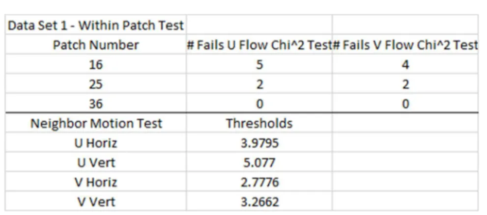
1. Table 1: Initialization of the Patch Number and Thresholds for Data Set 1 ... 42
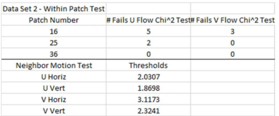
2. Table 2: Initialization of the Patch Number and Thresholds for Data Set 2 ... 43
3. Table 3: Initialization of the Patch Number and Thresholds for Data Set 3 ... 43
4. Table 4: Initialization of the Patch Number and Thresholds for Data Set 4 ... 43
LIST OF FIGURES
1. Figure 1: Algorithm Flowchart ... 22
2. Figure 2: Histogram Equalization Results ... 24
3. Figure 3: Convolution Demonstration ... 25
4. Figure 4: Original Image – Low and High Threshold Edge Detection ... 26
5. Figure 5: Optical flow of 2 Image Frames with Pixel Points Velocity Estimation .. 27
6. Figure 6: Image Derivatives in the X (left) and Y (right) Directions ... 28
7. Figure 7: Barber Pole Illusion with True Motion and Incorrect Optical Flow ... 28
8. Figure 8: Iterative Refinement of Optical Flow using Image Pyramids ... 30
9. Figure 9: Image 1 ROI with Corners from Frame 1 (Dot) and Frame 2 (Plus) ... 31
10.Figure 10: Graphical Representation of an Integral Image ... 33
11.Figure 11: 9x9 Box Filters for Convolution with Image to Approximate Gaussian . 34 12.Figure 12: Increase in Scale of Filter using Integral Images Reduces Computation . 35 13.Figure 13: Fast-Hessian Detection of Feature points in an Image ... 35
14.Figure 14: Haar wavelet x and y and Orientation Assignment Calculation ... 36
15.Figure 15: Feature Extraction Process to Build Descriptor ... 37
16.Figure 16: Bright-on-dark and Dark-on-bright would not be matched... 37
17.Figure 17: SURF Matched Features for Two Upright and Rotated Frames ... 38
18.Figure 18: Example Homography transform between two planes x and x’ ... 40
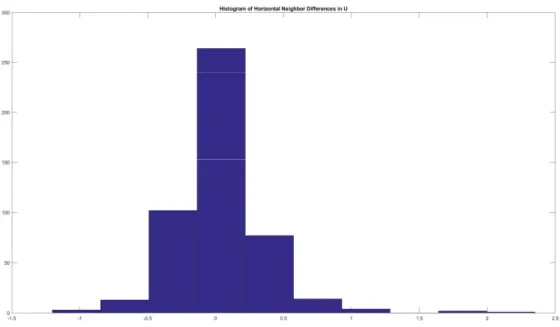
19.Figure 19: Data Set 1 Histogram of U Patch Neighbors Horizontal Direction ... 44
20.Figure 20: Data Set 1 Histogram of U Patch Neighbors Vertical Direction ... 44
21.Figure 21: Data Set 1 Histogram of V Patch Neighbors Horizontal Direction ... 45
23.Figure 23: Data Set 2 Histogram of U Patch Neighbors Horizontal Direction ... 46
24.Figure 24: Data Set 2 Histogram of U Patch Neighbors Vertical Direction ... 46
25.Figure 25: Data Set 2 Histogram of V Patch Neighbors Horizontal Direction ... 47
26.Figure 26: Data Set 2 Histogram of V Patch Neighbors Vertical Direction ... 47
27.Figure 27: Data Set 3 Histogram of U Patch Neighbors Horizontal Direction ... 48
28.Figure 28: Data Set 3 Histogram of U Patch Neighbors Vertical Direction ... 48
29.Figure 29: Data Set 3 Histogram of V Patch Neighbors Horizontal Direction ... 49
30.Figure 30: Data Set 3 Histogram of V Patch Neighbors Vertical Direction ... 49
31.Figure 31: Data Set 4 Histogram of U Patch Neighbors Horizontal Direction ... 50
32.Figure 32: Data Set 4 Histogram of U Patch Neighbors Vertical Direction ... 50
33.Figure 33: Data Set 4 Histogram of V Patch Neighbors Horizontal Direction ... 51
34.Figure 34: Data Set 4 Histogram of V Patch Neighbors Vertical Direction ... 51
35.Figure 35: Data Set 5 Histogram of U Patch Neighbors Horizontal Direction ... 52
36.Figure 36: Data Set 5 Histogram of U Patch Neighbors Vertical Direction ... 52
37.Figure 37: Data Set 5 Histogram of V Patch Neighbors Horizontal Direction ... 53
38.Figure 38: Data Set 5 Histogram of V Patch Neighbors Vertical Direction ... 53
39.Figure 39: Data Set 1 Tracking Results Frame 1, 2, 1537 to 1538-1540 ... 55
40.Figure 40: Measured U Optical Flow vs Corrected Flow by Neighbors ... 56
41.Figure 41: Measured V Optical Flow vs Corrected Flow by Neighbors ... 57
42.Figure 42: Frame 1768 Occlusion... 58
43.Figure 43: Data Set 2 Tracking Results Frame 1, 2, 1607 to 1608-1610 ... 59
44.Figure 44: Measured U Optical Flow vs Corrected Flow by Neighbors ... 60
46.Figure 46: Data Set 3 Tracking Results from Frame 1, 2, 191 to 192-194 ... 62
47.Figure 47: Measured U Optical Flow vs Corrected Flow by Neighbors ... 63
48.Figure 48: Measured V Optical Flow vs Corrected Flow by Neighbors ... 64
49.Figure 49: Data Set 4 Tracking Results from Frame 1, 2, 2354 to 2355-2357 ... 65
50.Figure 50: Measured U Optical Flow vs Corrected Flow by Neighbors ... 66
51.Figure 51: Measured V Optical Flow vs Corrected Flow by Neighbors ... 67
52.Figure 52: Data Set 5 Tracking Results Frame 1, 2, 2321 to Frame 2322-2324 ... 68
53.Figure 53: Measured U Optical Flow vs Corrected Flow by Neighbors ... 69
54.Figure 54: Measured V Optical Flow vs Corrected Flow by Neighbors ... 70
55.Figure 55: U and V Flow Over Five Heart Cycles – Data Set 1 ... 71
56.Figure 56: U and V Flow Over Five Heart Cycles – Data Set 2 ... 72
57.Figure 57: U and V Flow Over Five Heart Cycles – Data Set 3 ... 73
58.Figure 58: U and V Flow Over Five Heart Cycles – Data Set 4 ... 74
LIST OF ABBREVIATIONS
WHO World Health Organization ... 1
ROI Region of Interest ... 1
CT Computed Tomography ... 3
MRI Magnetic Resonance Imaging ... 3
SPAMM Spatial Modulation of Magnetization ... 3
CSPAMM Complementary Spatial Modulation of Magnetization ... 3
SA Short-Axis Slice ... 3
LA Long-Axis Slice ... 3
RF Radio Frequency ... 3
HARP Harmonic Phase Algorithm... 5
LK Lucas-Kanade Optical Flow ... 5
HS Horn-Shuck Optical Flow ... 5
LKD Lucas-Kanade-Dense Optical Flow ... 5
PDE Partial Differential Equation ... 6
LV Left Ventricle ... 6
RV Right Ventricle ... 6
ARMC Active Relative Motion Cancelling ... 7
POI Point of Interest ... 8
TPS Thin-Plate Splines Model ... 10
EKF Extended Kalman Filtering ... 10
SIFT Scale-Invariant Feature Transform ... 12
KLT Kanade-Lucas-Tomasi ... 21
SURF Speeded Up Robust Features ... 23
CHAPTER 1: INTRODUCTION
Cardiovascular diseases are defined by the World Health Organization (WHO) as a group of disorders of the heart and blood vessels that restrict blood flow to a specific region. These diseases are also labeled as ischemic disorders that include coronary heart disease, peripheral arterial disease, and deep vein thrombosis. The disorders classified can lead to severe conditions that include myocardial infarctions, heart failure, strokes, and more. Cardiovascular diseases are the leading cause of death globally, and an estimated 17.5 million people died from these diseases in 2012 (WHO, 2016). Cardiac motion must be monitored non-invasively for the
assessment of cardiovascular function using motion tracking systems and medical imaging data. The non-invasive tracking systems must be able to model and predict the movement of structures of the heart muscle, and analyze their movement overtime for applications that include
diagnostic analysis.
Computer vision techniques have been widely used in the medical field to develop algorithms for these applications. For example, post-processing techniques have been used to improve the quality of images and to extract information. Some of these algorithms have been implemented in software to improve the overall image intensity, to analyze specific regions of interest, or to take measurements for accurate analysis and diagnosis (Najarian & Splinter, 2012). Some of the existing cardiac motion tracking techniques estimate the movement of structures of the heart muscle by using a specific model to predict this motion. Cardiac motion tracking by this approach requires a priori understanding of the motion. Since the motion of the heart could change over multiple heart cycles, the models developed could fail to account for this change, which makes it difficult to recover from tracking failures. The research presented in this work will aim at improving the heart motion tracking algorithms.
The purpose of this research is to develop the algorithm and software, by using computer vision techniques, to continuously track the motion of a biological heart from two-dimensional imaging data without using a motion model. The non-parametric motion tracking algorithm will be used to estimate the motion of non-rigid structures of the heart by tracking point features identified in a user-defined local region of interest (ROI), on or within the heart. The algorithm will be developed using multiple computer vision techniques, including, but not limited to, feature extraction, matching, motion estimation, and outlier detection techniques. It is fully
2
realized that point feature-based tracking methods could potentially be disrupted by large motions, noise, lost frames or occlusions. It is important for a tracking system to have the capability of detecting such conditions. In this method, the tracking quality of these point features will be quantified by evaluating the consistency in frame. If the tracking quality fails a set of criteria, the algorithm is able to flag the failure of tracking. Future, it will be able to realign with the motion and recover from the failure. Finally, it is purely based on two-dimensional imagery data, and is thus considered a non-invasive approach.
The developed algorithm from this thesis can be utilized in many other applications. For example, the movement of myocardial walls or blood vessels could be tracked continuously to assess function by analyzing the motion and strain fields of these structures. Another possible application for this algorithm could be long-term single-cell tracking, which could improve the analysis of the cellular dynamics of a specific cell line. Current research in this field looks to improve upon the lack of software techniques in single-cell tracking, and reduce the amount of data acquisition needed (Hilsenbeck et al., 2016). Since cells move as non-rigid bodies, the developed algorithm can be used in this application to highlight and continuously track a specified cell for analysis. Since most tissues and organs that make up the human body are non-rigid structures that need to be tracked continuously, an additional application for this algorithm could be in the diagnostic analysis of other structures using imaging modalities. If a
measurement is to be acquired using a specified imaging technique, the algorithm will be able to track the non-rigid motion of a region to provide the supplemental geometry for continuous data acquisition.
The algorithm proposed in this thesis improves the existing techniques because 1) it does not require underlying motion model to be known, 2) it quantifies the current tracking estimate, and 3) it can recover from a failed tracking estimate. Chapter 2 will review the current motion tracking techniques that are applicable to biomedical systems and estimating cardiac motion. The underlying methods used for algorithm development and the experimental design will be
presented in chapter 3. Lastly, the results of the tracking algorithm, discussion and a conclusion will be presented in chapters 4, 5, and 6 respectively.
CHAPTER 2: REVIEW OF THE LITERATURE
The literature review will focus on three areas. The first focus is on the research related to heart motion estimation and modeling using medical imaging data. The second part of this review is focused on motion tracking models developed for robotic-assisted surgery applications. Finally, the existing approaches that are related to the proposed algorithm of tracking non-rigid motion, such as piece-wise tracking, will be discussed.
2.1: Medical Image Tracking: MRI Tagging
Different imaging modalities, such as CT, MRI, and ultrasound, have been used as diagnostic tools to monitor patient cardiac function and analyze cardiac motion to improve diagnosis. MRI tagging has been a useful procedure to obtain detailed information to track the motion and strain fields of myocardium. MRI tagging was introduced in the late eighties, when Zerhouni et al. developed a technique for generating visible image markers to tack myocardial movement without the need for physically implanted markers (Zerhouni et al., 1988). Two of the most popular MRI tagging techniques used today are the spatial modulation of magnetization (Axel & Dougherty, 1989) and complementary spatial modulation of magnetization (Fischer et. al, 1993) labeled as SPAMM and CSPAMM respectively. Both techniques generate a grid pattern across the images for cardiac motion analysis. SPAMM generates this tag pattern through selective radio frequency (RF) pulses throughout the cardiac cycle, while CSPAMM improves upon this technique to reduce fading of the tag pattern and improve the signal-to-noise ratio (Ibrahim, 2011). Research has been completed on the development of automated tools and tracking models to assist clinicians with cardiac motion diagnosis, and three different examples of these tools will be discussed further.
In a study conducted by Chandrashekara et al. (2003), a statistical model of the myocardium motion field of several healthy volunteers’ tagged MRI data was developed and tested. The objective of this research was to use prior information to develop a statistical model to track the motion of myocardium from patient data. To develop the statistical model, data from 17 volunteers, consisting of short-axis (SA) and long-axis (LA) slices, was acquired. Also, a cine breath-hold sequence of data was taken to develop a SPAMM tag pattern at the end of expiration for generating a grid pattern across the images to analyze motion (Chandrashekara et. al, 2003).
4
With the MRI tagged data collected, a statistical model was generated from all image frames between end-diastole and end-systole using all seventeen patients. Both the SA and LA data was used to derive a myocardial motion field for all individual subjects, and to account for the twisting, contraction, and shortening of the heart. The SA and LA images acquired were re-sampled by ordering images such that the first frame is aligned with end-diastole, or relaxation. With the images re-sampled to follow the cardiac cycle, a transformation function was derived to estimate the movement of any point in the myocardium at each frame. The actual motion fields for each image were then calculated by transforming multiple points within one image frame to estimate the position of those points in the next frame, and subtracting transformed position with the actual location in the current frame. The motion fields were computed to model the
deformation of the heart within the image throughout time. Next, the motion fields of each data set were mapped temporally and spatially to a reference subject. This was done to develop a common coordinate system for points within each image and develop a common time scale for all image frames. With the common coordinate system developed, principal component analysis was conducted to build the statistical model for the cardiac motion. Two separate models were built and validated by tracking the motion of the heart in eight separate data sets for all time frames of the cardiac cycle. Both models differed in specific parameters, but the displacement of tag intersection points was compared to the displacement of these points measured by a human observer for each model. The root-mean-square tracking error was found to be below 2
millimeters for the cardiac cycle over all eight data sets, which is labeled as a good performance for motion tracking (Chandrashekara et. al, 2003).
The results of this study show that the cardiac motion can be modeled and applied to different data sets to track the motion of intersecting lines, or deformations, from tagged MRI data with a small displacement error. It further shows that the heart motion can be modeled and tracked overtime. The model was not optimal for real-time tracking, as it does not account for the variability of the heart rate over multiple contraction cycles. Improvements to the model could be made to account for the variation from changes in the motion pattern of different healthy and diseased patients. The method proposed in this study also requires the use of tagged MRI images, which increases data acquisition cost. The model was also not developed for applications that require tracking recovery from lost data or occlusions.
5
In a study conducted by Hassanein et al. (2014), a mathematical model was generated to test tracking methods of cardiac motion with synthetic images, to model left ventricular function of tagged MRI data. The synthetic data was modeled as a circular disc with an inner radius of 30 millimeters and outer radius of 40 millimeters to simulate the endocardium and epicardium. The displacement model varied over polar coordinates, where the radius decreased to a specific point and then increased to simulate the contraction and relaxation of the cardiac cycle. The polar coordinates were then transformed into a Cartesian system to develop a sequence of test images. Using a known model, the SPAMM and CSPAMM tag patterns were overlaid on the image to simulate actual tagged data. To complete the synthetic data, Gaussian white noise and
exponential decay of the tag line amplitude was applied to simulate actual noise artifacts from real time imaging. The synthetic data set motion was then tracked overtime by comparing optical flow techniques with a commercially utilized HARP technique. The harmonic phase algorithm (HARP) is a commercially available MRI analysis technique to process the motion of tagged MRI data (Hassanein et. al, 2014).
Image tracking techniques based on optical flow were applied to the synthetic data set, along with HARP to estimate the motion of the circle over time. Optical flow is a computer vision technique to track the change in pixel motion overtime. Optical flow can be defined as the two-dimensional displacement or velocity estimation of pixel patches on an image plane. Three different optical flow techniques Lucas-Kanade (LK), Horn-Shuck (HS), and Anisotropic LK (LKD) were used in this study. The radial strain and estimation errors were calculated over each image frame for all four methods, and the radial strain was compared to the actual strain
measured from the image sequences. The results show that the LK method produced the most accurate strain measurement at the epicardial or border of the circle for tag patterns, and produced the smallest tracking error overall for all tests. The commercially available method, HARP, was found to have good tracking accuracy in the endocardium or inner circle, but failed to track the border of the circle for both tag patterns. The HS results were found to have the greatest tracking error among optical flow techniques, but performed better than the HARP method at the border. The LKD tracking error was found to be similar to that of the LK method at the border, but was greater at the inner circle than the LK error (Hassanein et. al, 2014).
6
In a similar study, Arif et al. (2014) proposed a method for tracking specific structures in cardiac MRI images by propagating a segmentation from one frame to another across a sequence of images. This study improved upon the partial differential equation (PDE) solutions of optical flow techniques with consideration of the fluid motion present in the heart. The researchers proposed a new boundary condition to solve the PDE of the tracking methods by changing them from a zero velocity to a value linked to the inside of the segmentation that is not zero. The mathematical model developed was then discretized to generate an algorithm to be tested. The developed method was applied to publicly available data sets, the MICCAI Left and Right Ventricle sets (LV and RV), and compared to the commercially available Medivisio
segmentation software. Both methods start with a user selected initial segmentation of each ventricle, and the segmentation is propagated separately to compare both techniques. Full heart segments were also selected to track the myocardium outer boundary, left ventricle, and right ventricle (Arif et. al, 2014).
The results show that the proposed technique from this study improves cardiac segmentation and propagation throughout the entire data set when compared to Medivisio segmentation, and requires no manual correction throughout the entire data set. For the LV, the proposed method included a more accurate boundary segmentation and motion compared to Medivisio. However, the main difference between the two can be seen in the RV data. The Medivisio segmentation would group noise artifacts and components outside the true boundary of the RV. This would lead to a correction by the user to delete extra unwanted pixels to continue tracking. The proposed method was not interrupted by these artifacts and kept an accurate
boundary segmentation close to the actual RV wall. When these techniques were applied to segment out multiple structures, the Medivisio method failed and consistently could not correct itself to keep the segment boundary equal to the actual movement of the LV, RV, and
myocardium wall. The proposed method accurately tracked the boundary of the segmented LV, RV, and myocardium wall throughout multiple cardiac cycles (Arif et. al, 2014).
By making improvements to the general optical flow techniques, the proposed method from this study demonstrated accurate segmentation and tracking results for LV, RV, and myocardial boundaries. The proposed technique was also developed to be computationally efficient because the changes made did not alter the computational time significantly, when
7
compared to traditional techniques (Arif et. al, 2014). The method did not even require specific MRI tagging, and was developed to be non-specific to any imaging modality. The method was not developed for real-time tracking as the experiments were conducted as post-processing techniques on MRI data that is publicly available and does not include interference or occlusions. The acquisition cost to use this technique for MRI data would lead to an expensive data
acquisition for non-invasive diagnosis.
In summary, MRI is one of the medical imaging modalities used to track the motion of specific components of the heart, which requires preprocessed (tagged) data and can only track the heart within one region, such as the left ventricle. The high cost associated with MRI tagged data promotes the use of other imaging methods in the development of a tracking algorithm for diagnostic applications. The tracking algorithms presented support the use of optical flow
techniques to estimate the motion of the heart and improve upon commercially available tracking software. However, the techniques developed are not robust to occlusions or other interferences and cannot automatically correct a failed tracking estimate for the use in real-time cardiac motion tracking.
2.2: Robotic Assistant Surgery Tracking
Open heart and specifically coronary artery bypass surgeries require surgeons to operate on blood vessels that constantly move and cause interference. Research has been conducted to improve the working conditions for surgeons during operation also by using computer vision techniques. The master-slave robotic systems, such as the DaVinci machine, have been improved to include mechanical motion synchronization of the surgical instruments with the beating heart to track, predict, and cancel out the cardiac motion. Active Relative Motion Cancelling (ARMC) is one method used to actively cancel out heart motion by tracking a point of interest on the heart surface to provide surgeons with a still view (Bader et. al, 2007). Three different research studies on the development of cardiac motion tracking systems for this application and their motion tracking technologies will be reviewed.
In a study conducted by Bader et. al (2007), a model-based approach was used to build an estimator to reconstruct multiple feature points from one image frame to the next, to predict cardiac surface motion. A testing model was developed with a circular pulsating membrane, paced between 0.5 and 2.4 hertz, and physical markers to track motion using a stereo camera
8
system. The motion behavior of the membrane was derived as a system of coupled linear partial differential equations, and converted into a lumped parameter system to estimate the solution of the model at a discrete time point. A Kalman filter was utilized to estimate the state of the lumped parameter system from the location of marked feature points on the membrane model. The location of these points was found through feature extraction from both cameras using an edge detection technique, specifically Canny edge detection (Canny, 1986). The predicted deflection of a series of points that did not include the labeled markers was compared to the actual measured deflection of the labeled points as the model was pulsed at a frequency of 0.653 hertz. The results show that the average prediction error (measured – prediction) was found to be equal to 1.39 millimeters (Bader et. al, 2007).
The model developed from this study demonstrates that the deflection of a circular membrane, which resembles cardiac motion in the z-axis, can be tracked through feature detection. This model also successfully tracked the changes in motion throughout time using non-invasive imaging data. It is reported that at some image frames the Canny edge features could not be found, which contributes to an increase in the prediction error. More research on the types of features to be selected, such as corners instead of edges, could provide a better tracking model to reduce loss from occlusions or other interferences. The membrane model should be tested in real-time on cardiac images to improve non-rigid tracking and be more applicable to robotic-assisted surgery applications.
In a research study conducted by Tuna et al. (2013), two least-square prediction
algorithms were created and tested to predict future position estimates of points of interest (POI) from the heart surface. In this study, the heart motion displacement of three calves was recorded using a sonomicrometer system, and imaging data was tested with the algorithms developed. Two piezoelectric crystals were placed near the coronary artery and along the side of the heart to measure displacement. A “one step motion” estimation algorithm was first developed to predict the current POI using the prior position in previous frames through a process of adaptive
filtering. Adaptive filtering adjusts the filter weights using a least squares method to allow the algorithm to constantly update based upon the most recent iteration. The second approach
developed uses a generalized linear predictor to independently estimate each point over the entire image. This second approach computes an estimation matrix at each iteration, which was found
9
to be approximately constant throughout all frames. Both algorithms were tested on the pre-recorded cardiac displacement data to track the heart over all image frames. The results of this study show that the generalized predictor root mean square position error was found to be much smaller than the one step estimation at a constant and varying heart rate (Tuna et. al, 2013).
The algorithms developed in this study show that a motion predictor can be developed to actively track specific regions of the heart even when the heart begins to contract at a higher rate. The motion predictors were successfully able to track the non-rigid motion of the heart using non-invasive cardiac imaging data. The predictors were, however, not developed to account for interferences or occlusions, which occur during surgery. It is important to note that even though the prediction algorithms can actively track regions when the heart rate increases, the algorithms cannot track these regions when an abrupt change in heart rate occurs. This abrupt change could be caused from an abnormal arrhythmia or myocardial infarction. The methods presented in this study are also not implemented in real time in an active surgical system.
In a third study, Richa et al. (2010) presented a robust method for estimating three-dimensional temporal and spatial deformation of the heart surface using stereo endoscopic images and computer vision techniques. This method, based on previous research with Thin-Plate Splines (TPS) models, was improved to accurately track large ROI on the heart surface even in the presence of occlusions or tracking failures. In their previous studies, the TPS method was developed to select control points from a reference image of the heart and utilize a warp function to map the control points and the ROI from one frame to the next. It is important to note that the control points are selected manually by the user in a reference image from regions of high texture, such as edges. This study was conducted to improve upon this method by adding the heart motion dynamics to support the tracking accuracy of the TPS solution. A heart motion model was developed based on time-varying Fourier series that is recursively estimated using an Extended Kalman Filter (EKF). This model will be used to reestablish the motion of the heart when a tracking failure occurs. The current algorithm from this study was re-organized to evaluate the quality of the tracking result at every iteration. In the evaluation step, the image alignment error and the estimated three-dimensional heart shape will be checked. If the error is found to be high, the EKF and Fourier series model will be used to restore the tracking of the selected ROI. The alignment error is evaluated by calculating the normalized cross-correlation
10
coefficient of regions of about 40x40 pixels surrounding each control point. If three of these points were found to be below a set threshold, the current tracking TPS model stops and
continues when the control points are visible. The three-dimensional shape analysis is evaluated by calculating the bending energy of the ROI. If the bending energy of any point within this region is greater than a specific threshold, the tracking is stopped and the motion is reestablished from the EKF model. The improved tracking algorithm was tested on human data that was pre-recorded from previous research studies (Richa et. al, 2011).
The algorithm from this study was tested on image sequence from an endoscopic coronary bypass surgery using the DaVinci surgical platform on a human subject. The data consisted of 32 seconds of colored imaging data with a total of 1600 images. Eight control points were selected on the reference image, the EKF was initialized, and the alignment error and bending energy thresholds were set at 0.60 and 0.14 respectively. The researchers note that the first tracking error within the ROI occurred around 3.16 seconds, and the previous method was not able to recover. The new method fixed the tracking error by 3.18 seconds using the predicted heart motion from the EKF and continued. Throughout the whole test, the tracking was
suspended for 13.69% of the total time duration. This lead to a computational delay of 800 ms total from tracking loss to reestablishment. The large duration of the delay was found to occur due to the poor prediction quality from abrupt cardiac frequency changes, but the region was successfully tracked throughout the entire sequence (Richa et. al, 2011).
The results show that the non-rigid motion can be tracked through EKF and Fourier series modeling for applications in real time robotic-assisted surgery. The authors of this study suggest that abrupt cardiac frequency changes can be accounted for by incorporating electrocardiogram (ECG) data. The ECG could be utilized to predict abrupt changes in the heart frequency to improve tracking quality (Richa et. al, 2011). However, more instrumentation must be added to the existing method to measure the ECG. The algorithm presented in this study demonstrated that the visual tracking system must be robust to occlusions for robotic-assisted surgery applications. A tracking validation step can also be developed using the normalized cross-correlation coefficient for feature tracking in cardiac motion data.
11
2.3: Computer Vision Tracking Algorithms for Non-Rigid Motion Tracking
Most of the computer vision techniques initially developed for object tracking and motion detection had an implicit assumption that the object to be tracked in an image was rigid. For biological systems, such as the heart, a tracking system must be able to accurately track and predict the stretching or dilating motion of non-rigid structures, such as a blood vessel. It must estimate these areas of non-uniform motion within one region, which is typically found on the heart. There has not been substantial development of closed-form tracking algorithms for non-rigid heart motion in the literature. However, this problem could be solved through a linearized, piecewise approach. Piecewise motion tracking is used to break up the motion field of a region into smaller areas, called neighborhoods, that can be estimated individually. The next set of studies will present techniques that can be used to model and estimate regions in a scene or image that have different motion fields.
In a study conducted by Cremers and Soatto (2004), a motion estimation and
segmentation technique was developed to track multiple regions of interest (ROI) and segment out objects from their respective motion field. This proposed method was developed using Bayesian inference that is updated based on continuous optical flow measures outlined by a contour representation of the motion of separate regions. The motion field is also optimized by a gradient descent minimization factor. The initial image frame is segmented into multiple regions of piecewise parametric motion, where the motion of each region is solved from a system of partial differential equations. With the equations and algorithm developed, this method was first tested on a set of synthetic gray-scale images of similar intensity where the ground-truth motion is known. The results of these tests show that the objects located within the image set were found to be accurately segmented based on their separate motion and not appearance. In a more
applicable test, a traffic scene test set was developed by setting an image of two cars to move toward the top-right of the image, while the background of this same image was moved to the bottom-left to simulate camera movement. The motion segmentation method was compared to a previously developed intensity-based segmentation technique for this image sequence. The results show that the intensity-segmentation was only able to segment out the bright and dark areas within the image. The proposed method was accurately able to segment out each individual car from the background, and obtain an accurate estimate of the motion of the cars and
12
traffic sequence of multiple moving cars and a moving background, and estimates the motion of a selected initial segment within the first image. It is important to note that in this test sequence, the ground-truth motion was not known. The results of this test show that the segmentation of one car in the scene was robust to competing motion of other cars and the background. The algorithm began to fail as the car started to move perpendicular to the viewing plane of the image. At this point the optical flow cannot be solved for, and this error is known as the aperture problem. The results of this study show that regions of separate motion can be estimated and the boundaries of these regions can be highlighted to segment out each moving object in a scene. The segmentation method was developed for piecewise motion fields based on parametric motion models. To segment regions of the moving heart, this model cannot be used. However, this technique could be utilized if the specific parametric motion from pre-segmented heart data is learned and used as an input to the motion segmentation algorithm (Cremers & Soatto, 2004).
In another approach proposed by Zhou, Yuan, and Shi (2008), an object tracking
technique was developed by combining the use of a scale invariant feature transform (SIFT) with a mean shift algorithm. This algorithm integrated two commonly used object tracking techniques to improve consistency in tracking performance, even if one of them were to fail. A SIFT feature detector is a method that locates points of interest that occur at the maxima and minima of a difference of Gaussian function, across all scale space. Local key points are identified through this step, and then a feature descriptor is developed for each key point to assign measures for robustness of the point against rotation or brightness changes. The final SIFT feature points are chosen by testing the robustness of each key point detected by building an image pyramid and re-sampling the points at each level of the image scale space. The mean shift algorithm works by conducting a color or intensity similarity search using color histograms across two image frames. An initial target window, with its position, is given in the current frame, and the algorithm begins to step through the next image frame in search for a confidence region that has a similar
histogram distribution. Both tracking techniques are used in this algorithm by taking measurements and developing an expectation-maximization scheme to achieve a maximum likelihood estimation of similar regions across multiple image frames. A region of interest, or rectangle, is defined in the first frame, along with the computation of the color histogram of this region and the SIFT features. Then in the second frame, the algorithm will examine surrounding areas of the initial position from the previous frame for color similarity measures along with the
13
sum of square difference between SIFT features. The expectation-maximization will then be used to locate regions that are similar while minimizing the distance between the detected locations from the mean shift and SIFT results. This process will then iterate until the difference between the two is smaller than a set threshold, and the target location will be found in the current frame. The algorithm was tested on four publicly available data sets, and then compared to the SIFT and mean shift detectors separately. The Euclidian distance between the object detection of the three techniques and the ground truth were then compared, and it was found that the mean-shift combination algorithm had a significant lower tracking error for both a single object in a dark scene and tracking a single object in a crowded scene. The combination of both techniques did, however, increase computation time when compared to running each
individually. Overall, the proposed algorithm shows promise in improving object tracking over multiple image frames in different scenarios by combining different object tracking techniques together to improve results (Zhou, Yuan, & Shi, 2008).
The combination of different tracking techniques shows an improvement in estimating the motion of one segment in a scene of competing motion. Even though the initial region of interest was assumed to be rigid in all the algorithms presented, this individual consistent tracking can be used for piecewise motion estimation by breaking up a non-rigid region into smaller areas that can be assumed to move as rigid segments.
A third study, proposed by Ren in 2008, improved optical flow results by developing an image-based grouping approach in motion estimation. This method begins by computing a soft edge and texture boundary map using a probability-of-boundary operator, which combines local brightness, color, and texture contrast and differs from traditional edge detection techniques. The boundary map will then be used to develop pairwise affinities between subsequent pairs of points through an intervening contour method. The affinity value represents if two points are separated by strong boundaries or if they belong in a uniform region. The image will then be sampled at corner or edge points for the affinity calculation step, and then the flow will be estimated at these sample points. The affinity values calculated will define a support for the spatial integration of flow to avoid connections across object boundaries, also known as a semi-local flow approach. An affinity-based optical flow will then be calculated across the image to estimate the motion of these points from one frame to the next. The grouping method was then tested on publicly
14
available data sets and the average angular error and average end-point error was compared with a top-ranking flow estimator from Black and Anandan (1996). The results show that the
grouping approach significantly improves the optical flow estimation by lowering both errors measured. These results can be contributed to the improved flow estimation for points that are close to boundaries in an image, but do not necessarily move in the same direction as the
boundary. While traditional flow estimators tend to group unwanted regions into areas of strong intensity, like edges and corners, even if the true motion of these points is in a different direction. The downfall to this approach is that the computation time increases due to the increase in the number of points used in computation of the flow field. These results show that grouping optical flow measures by edges or corners improves tracking estimation. This grouping approach can be useful for piecewise estimation as well to estimate regions that undergo non-rigid motion similar to cardiac motion (Ren, 2008).
In summary, existing heart motion tracking systems from imaging modalities were found to be accurate only at specific locations on or within the heart. The systems reviewed here require tagged MRI data, a prior model, or a lot of prior imaging data that can be expensive to capture and have long computation times. Non-invasive optical imaging tracking techniques could improve upon MRI tracking systems presented because optical techniques require less exposure time, are less-invasive, and are more cost effective. The data used to develop this algorithm stems from optical imaging techniques, but could also be used in other imaging modalities. Tracking systems used on robotic surgery applications were found to be accurate. However, these algorithms require the use of artificial sensors and computationally expensive models to effectively track the motion of the heart. Lastly, a set of computer vision techniques that were not originally developed for tracking non-rigid biomedical systems could be used to solve for piecewise motion estimation. Overall, there exists a gap between existing systems and the need of a heart motion tracking approach that is continuous, non-parametric, and robust to tracking failures.
CHAPTER 3: METHODS 3.1: Non-Rigid Motion Observation Model
In order to continuously estimate the non-rigid motion of a biological system, such as the heart, a traditional computer vision technique that assumes a rigid body is no longer directly applicable. A piecewise tracking algorithm is proposed here. It will break up a ROI into smaller components, each estimated as a pseudo-rigid segment. Each small component will be estimated as a pseudo-rigid segment because not every point within that segment will follow the same exact motion. The motion of some points will differ slightly, but the distribution of this motion will follow an approximately rigid model. All the segments combined can approximate the non-rigid motion of a ROI as observed in a two-dimensional space (image).
In order to introduce the piecewise algorithm, a body frame and a camera frame are defined in a three-dimensional space. The body frame is a three-dimensional Cartesian
coordinate system attached to the target biological system (the heart), with an arbitrarily chosen origin point (j). If the heart were a rigid body, another point (i) can be defined at a fixed location in the body frame, , which does not change over time in a rigid body frame. However, in a non-rigid system, the location of this point becomes a function of time, i.e. ( ). At a specific time ( = ), the location of this point would be at ( ). Since the point (j) is the origin, the location of this point in the body frame is zero, i.e., = 0, regardless of time.
The camera frame is another rigid 3D Cartesian coordinate system. At a time , the origin of the camera frame is located at, for example, ( ), which is a location observed in the rigid body frame. The coordinates of the point (i) and the origin (j) in the camera frame is thus defined by equation 1 and 2 respectively:
( ) = ( )[ ( ) − ( )] (1)
( ) = ( )[ ( ) − ( )] (2)
where is the rotational transform of a point from the body frame to the camera frame. Thus, ( ( )) represents point i observed in the camera frame at time .
16 3.1.1: Piecewise Approximation
Now let the time stamp step from to , still in a non-rigid system. If a rigid body had been assumed in a predictive model, it would not agree with the actual observation. The error (ϵ) between the predicted location and truth is described in equation 3, where ( ) stands for the prediction.
= − ℎ = ( ) − ( ) (3)
Both terms can be substituted from equation 1 and simplified below in equation 4:
= ( ) − ( ) − ( ) − ( ) (4)
As afore mentioned, in a non-rigid system, ( ) ≠ ( ). We further assume that the location of point (i) has been biased through deformation by ∆ , such that
( ) = ( ) + ∆ The prediction error is therefore also a function of ∆ :
= ( ) − ( ) + ∆
where is the rotation transform from the body frame to the current camera frame. We can then simplify the equation above into:
= − ∆ (5)
The difference between the rigid and the non-rigid motion is now observed in the camera frame, as shown in equation 5. In a non-rigid system, the bias ∆ can be defined as a function of time and space shown in equation 6 below:
∆ ( − , − ) (6)
In a piecewise approach, the non-rigid motion will be approximated with pseudo-rigid motion in a small neighborhood, which is observed as a small “patch” in this image. In order for this approximation to be sufficiently accurate, a constraint must be applied to ∆ such that it can be linearized. In general, the bias term is assumed to be continuous over time and space in a biological heart. The bias term must fit the continuity constraint as described below:
17
∆ − , − is smooth if ∆ , ∆ exist and are continuous For this function to be smooth, it must be differentiable in time and space everywhere in its domain. Also, all the partial derivatives must exist and be continuous in all orders across the domain. For the function to be continuous, it must be defined at any point, and the value at that point must equal a real number. The limit of the function must also exist and be equal to the function value at that point.
∆ is a function of time and space because its value will change overtime, or consecutive image frames, and at different points in the ROI. The bias within a small patch can be
approximated using first order Taylor series and is shown below in equation 7:
∆ , ≅ ∆ , + (∆ ) + (∆ ) + (∆ ) + (∆ ) (7)
where ∆ is the change in time from to and (∆ , ∆ , ∆ ) represents changes along the three axes in the body frame. To further simply the analysis, in equation 8, we assume that the bias is only sensitive to the distance between two points, such that
∆ , ≅ ∆ , + (∆ ) + (∆ ) (8)
where ∆ is the change in distance from a point (i) to the origin (j) within one patch. Since the bias is assumed to be continuous and smooth, if the change in time between image frames is approximately small (∆ ≅ 0), the bias due to the time change will be sufficiently small. The bias within a patch due to distance can then be defined by evaluating equation 8 using the distance variable only:
∆ , ≅ ∆ , + (∆ )
Similarly, there would exist a small neighborhood surround the origin (j), in which any point (i) has | | ≅ . In other words, there is a pseudo-rigid relationship between both points. This neighborhood, will be called a “patch” in this work. If a patch was observed to be approximately rigid at a time ( ), it still will be approximately rigid at the next time step ( ). Therefore, the bias change due to time will be minimal, i.e., ∆ , ≅ ∆ , .
18
Piecewise motion estimation also requires a constraint across neighboring patches. Neighboring patches do not necessarily share the same linear transformation. However, their motion models are expected be continuous. Assume that a point (k) is located in a patch adjacent to the one defined with origin (j). The bias term at point (k) can be approximated with a first order Taylor series following equation 9 below:
∆ , ≅ ∆ , + (∆ ) (9)
The variation over time is assumed to be negligible. Both patches will follow a pseudo-rigid model. Since ∆ is smooth, the first order Taylor series is sufficient to estimate the bias if the distance between both points (∆ = − ) is small enough. It provides yet another constraint on the patch size. With smaller patches, the bias ∆ between neighboring patches would have a limited difference shown in equations 10 and 11 below.
∆ , − ∆ , < (10)
In other words,
( ) − ( ) − ( ) − ( ) < (11)
3.1.2: 2D Observations and Constraints
The non-rigid motion of point (i), is observed in a two-dimensional space (image). First, the location of this point can be converted from body frame to camera frame, as afore mentioned:
( ) = ( )[ ( ) − ( )]
( ) is defined in the three-dimensional camera frame, with x, y, and z components: ( ) = [ , , ]. Conventionally, x points to the right, y points down and z points out of the camera lens. The location of (i) will be observed in an image that has normalized x and y
components, which will then be compared to the predicted location of this point as shown below (Hartley & Zisserman, 2004):
: ( ) = , : ( ) =
19
The prediction, once again, is assumed to follow an approximately rigid model. If the observed location in (x, y, z) is approximately equal to the prediction in ( , , ̂), i.e. ∆ ~0, then the prediction is accurate and the tracking error (ϵ) could be minimized. It is important to note that the z component represents the distance from the camera frame to the body frame. In a medical imaging system, the distance between the camera and target is unlikely to dramatically change. Therefore, z is assumed to be approximately equal to the predicted ̂ in both locations ( ≅ ̂). We assume that the majority of motion will be observed in the x and y directions.
Constraint 1: Within a patch that is sufficiently small, the pseudo-rigid prediction is expected to agree with observation
= − ℎ ≅ 0
( ) ≅ ( )
Any disagreement would be attributed to noise in feature tracking, which is expected to follow Gaussian distribution. As to be discussed in the following sections, motion of a pseudo-rigid patch can be modeled by a linear transform, such as the fundamental matrix or a homography matrix. It allows us to predict the motion of any single point based on the consistency of neighboring points. Furthermore, since we assume that the 3D motion between neighboring patches would have a limited level of difference, the difference in 2D motion would also be limited.
Constraint 2: When the difference between the neighboring patches is sufficiently small,
( ) − ( ) − ( ) − ( ) <
It is realized that the difference is unknown and will differ over location and time. However, when observed over a large number of points over time, it is assumed to follow a Gaussian distribution between two patches. The quality of non-rigid motion tracking can be quantified by how well the tracking residuals can meet this criterion.
3.1.3: Configuration of Piecewise Tracking
The first constraint assumes that the motion within a patch is approximately rigid, and in that case, the tracking residuals will be dominated by noise. We assume that with the right patch
20
size, these residuals will follow a normal distribution with the number of outliers no greater than two sigma or be greater than five percent of the motion within a patch in the x and y directions. This pseudo-rigid motion can then be estimated with all the point features observed in this patch, through a computer vision technique such as a homography or averaged optical flow estimation. The second constraint assumes that neighboring patches are interconnected, and that the motion from patch to patch is continuous. The second threshold will be determined by sampling the motion, both in the x and y directions, at every patch through a set number of image frames. The motion differences between neighboring patches in the same row and column will also be calculated. The motion across neighboring patches will also be assumed to follow a normal distribution. This assumption will be confirmed through a chi-square goodness of fit test of the motion differences between neighboring patches. The motion differences at every patch with its corresponding neighbors across a set number of image frames will be collected to estimate the mean and standard deviation. The mean plus two sigma, or 95th percentile point, will be calculated for every distribution, and the maximum value among all distributions will then be used as a threshold. Four difference thresholds will be calculated in total. The first two are the horizontal and vertical differences for the motion in the x-direction, and the next two as the horizontal and vertical differences in the y-direction. Each motion difference will be compared against the corresponding threshold, and will be flagged if it exceeds the threshold.
For every individual patch, both constraints are checked at every frame to quantify the quality of motion prediction. If either constraint is not met, the tracking estimate is potentially incorrect and will be flagged. If the constraints are still not met two more times in a row, it is considered a tracking failure, and reinitialization step must be completed among the discontinued image frames to restart the piecewise tracking process.
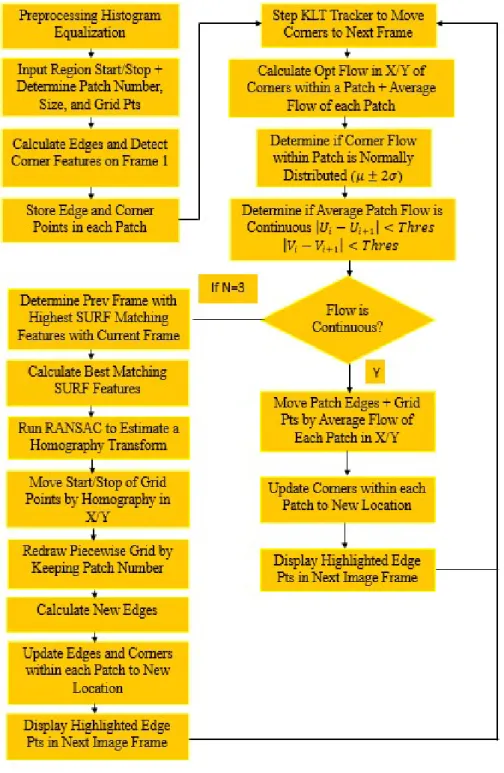
The algorithm has been illustrated in a flowchart, as shown in Figure 1 below. The flowchart presents an outline of the necessary steps to track an input region selected from the user, and estimate the motion at every image frame. The algorithm will begin by preprocessing the image data set through histogram equalization to improve the overall contrast of the image. The user will then be asked to input the starting and stopping point to define a region of interest to be tracked. Next, the appropriate size, number of patches, and the motion difference thresholds will be determined. The appropriate edges and detected corner features will be then stored in
21
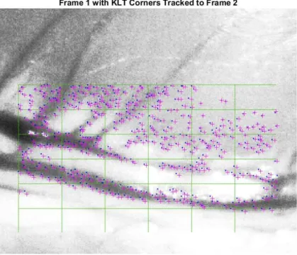
each patch from frame one, in the next step, to be used as the initial frame in tracking. A Kanade-Lucas-Tomasi (KLT) optical flow approach will then be used to move corner features from the previous frame to the current frame to be used as an optical flow measure for the ROI (Shi & Tomasi, 1994). The next major component of this algorithm will be to check the quality of tracking by determining if the flow within a patch is normally distributed, and check if the average flow measure between neighboring patches is continuous. If the quality of tracking passes this set of criteria, the edges from the previous frame will then be moved by the average optical flow measure of each patch. If the quality of tracking was found to fail either set of criteria, this frame will be flagged. If a continuous failure is found for up to three flags, the reinitialization step will follow. For the reinitialization step, a homography transform will be used to realign the piecewise grid and relocate the features to be tracked. Highlighting the edge points moved to the next image frame will also provide qualitative results to determine if the non-rigid region is accurately tracked as pseudo-rigid patch segments. The algorithms used in each component of this flowchart will be presented in detail in the following section.
22
Figure 1: Algorithm Flowchart 3.2: Computer Vision Techniques
The algorithm has been developed using multiple computer vision techniques and has been implemented in MATLAB. The following sub-sections will introduce the theory, implementation, and simulated results to show how each technique works in relation to the
23
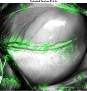
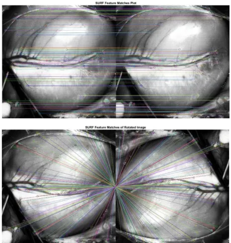
overall process. Section 3.2.1 will present the preprocessing equalization, edge detection, and calculation to determine the appropriate patch number and size. Section 3.2.2 will present the corner detection step, motion estimation or optical flow technique, and the quality of flow estimation steps. Section 3.2.3 will define the use of Speeded Up Robust Features (SURF) in determining matching feature points between two discontinued image frames. This section will then continue to outline the Random Sample Consensus (RANSAC) process using these SURF feature points to estimate a homography transform to reinitialize the piecewise tracking process. 3.2.1: Preprocessing: Histogram Equalization, Determine Correct Patch Size, Edge Detection
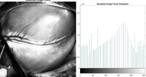
The initial data from the imaging system must be preprocessed to improve the overall visual quality of the images acquired. A histogram equalization function will be applied on every image as the first component of the algorithm. This function will first evaluate the intensity distribution, or histogram, from one or a few images. The normalization process maps a given distribution to another wider and uniform distribution so that the intensity values are spaced out over the entire range (MathWorks, 2017). This MATLAB function works by taking the
cumulative distribution function of the image intensity values and performing a transform to develop a linearized cumulative distribution function of the original image. The linearized distribution can be mapped back into an image that will have improved contrast and a spaced-out histogram. Figure 2 below demonstrates the histogram equalization process for two images of one of the heart data sets.
24
Figure 2: Histogram Equalization Results – Original Image and Respective Histogram (top) Equalized Image and Histogram (bottom)
The next step after histogram equalization is to determine the correct number of patches and the size of each at the beginning of the tracking process. To determine the correct number of patches, a separate function was developed to estimate the quality of the motion between the first two frames by searching for the optimal setting for the number of patches. The motion estimation technique is based on corner feature tracking within each patch, and will be described in the next section. Each patch will be evaluated on the bias against both constraints: the motion within a patch must be assumed to be rigid, and the motion across neighboring patches must be
continuous. To fit the first constraint, the motion within each patch will be tested for normal distribution through a chi-square goodness of fit and outlier detection tests. The motion between neighboring patches will also be tested to fit a normal distribution in the horizontal and vertical directions by using a chi-square goodness of fit test. A maximum threshold of each neighboring difference will then be calculated to represent the maximum offset allowed for motion among neighboring patches in either the x or y directions, as pointed out in constraint two of the piecewise tracking approach.
Edge detection is a key component in the tracking algorithm because locating the boundaries found within an image can provide the most useful information to identify a ROI. This technique will be used also as a preprocessing step to define the initial boundary points of the ROI within each patch. An edge can be defined as a transition point of the gray or pixel level of the image as it changes from an area of low values to high values or vice versa (Phillips,
25
2000). The edges of an image must first be detected to determine the main components of the image and provide information from the image. An image array mask is combined with the original image array data to detect and highlight the edges through a process called convolution. The output array data from this convolution will result in a reduction in overall noise of the image, and show the outline of the objects represented in the image. A correlation kernel, also known as a mask, can be convoluted with the original image pixel matrix data. The convolution operation can be shown in the demo provided by Figure 3 (Gimp, 2017). The resulting output image is the weighted sum of neighborhood input pixels from this function.
Figure 3: Convolution Demonstration
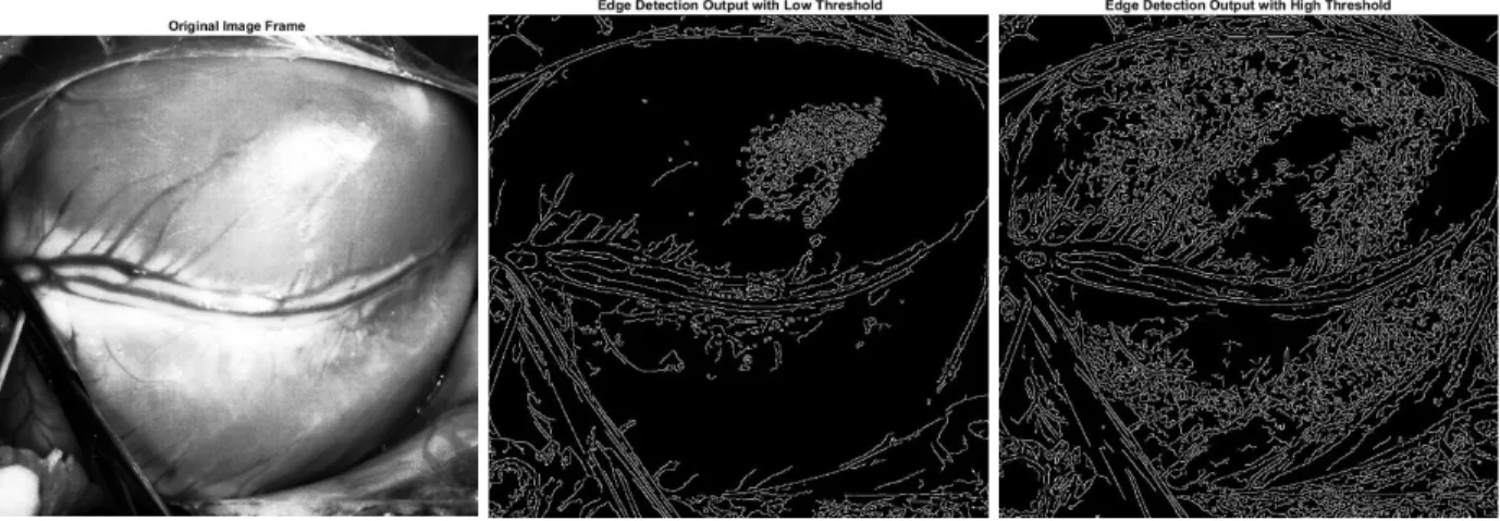
An image matrix is illustrated on the left side in Figure 3. Each pixel is marked with its intensity value, and the center pixel is outlined in red. The kernel is then applied to the area that has a green border. In the middle is the kernel matrix and, on the right, is the convolution result. The initial pixel intensity (70) has become 60: (61*0) +(60*1) +(64*0) + (66*0) +(70*0) +(75*0) + (70*0) +(76*0) +(78*0) = 60. As a graphical result, the initial pixel moved a pixel downwards. This convolution process is applied to locate the edges using a mask with specified values that can be changed. Figure 4 below shows the original image with the edge detection output images for a low threshold and high threshold. A canny mask is applied to the image using the
MATLAB edge function, where the strength of the mask can be tuned by decreasing the
threshold parameter (Canny, 1986). Increasing the threshold value, will lead to a decrease in the amount of edges detected. The edge detection algorithm must be tuned based on the application. With the edge locations known, each edge will be moved and highlighted from frame to frame based on optical flow or homography estimation.
26
Figure 4: Original Image (left) with Low Threshold Edge Detection (middle) and High Threshold Edge Detection (right)
3.2.2: Corner Detection and Kanade-Lucas-Tomasi Tracking (KLT)
With the image pre-processing and initialization steps completed, the ROI motion can be estimated. There exist multiple methods to estimate an object’s motion. A commonly used method is to solve for the optical flow of the object. Optical flow can be defined as the two-dimensional displacement or velocity estimation of pixel patches on an image plane. Figure 5 below shows an example of optical flow between two video frames (t and t + 1) with pixel points ( , , ). Computing the optical flow of the two frames of this video sequence results in velocity vectors ( , , ) to estimate the apparent motion of these points.
27
Figure 5: Optical Flow of 2 Image Frames with Points (left) and Velocity Estimation (right) The common optical flow techniques developed must define some assumptions and constraints to estimate the motion of points within an image. One important assumption is that the brightness (intensity) of a point remains constant from one frame to the next, even though the position of that point changes (Cremers & Wedel, 2011). The brightness constancy constraint is also labeled as the optical flow constraint, and is shown in equation 12 below.
+ + = 0 (12)
Where , , are the partial derivatives of the image with respect to x, y, and t. While u and v are the motion vectors in the x and y direction, respectively, that are to be estimated. Figure 6 below will show example images of the image partial derivatives in the x and y directions by applying an image gradient. Another optical flow assumption is spatial coherence, where neighboring points in an image frame typically belong to the same surface and have similar motions between image frames. A third optical flow assumption is temporal persistence, where the motion of an object, or group of points, within an image changes gradually over time. In the case for most optical flow approaches, the apparent motion of the points within an image frame is assumed to be small throughout subsequent frames. Regions within the image for optical flow movement must also avoid “bad” textures that include homogenous intensity values and areas of
28
linear symmetry. A classic example of the linear symmetry problem is the barber pole illusion shown in Figure 7 below. The true movement of the stripes within the image is horizontal, however the optical flow and perceived motion is that the stripes are moving up along the z-axis. Two additional constraints are typically added to solve this problem. The flow field is assumed to be smooth locally, and the optical flow is solved within a specific size window that is swept over the image to estimate the true motion. The barber pole illusion can then be solved along the outside edge where it is estimated that the information within the image is moving horizontally.
Figure 6: Image Derivatives in the X (left) and Y (right) Directions
Figure 7: Barber Pole Illusion with True Motion (middle) and Incorrect Optical Flow (right) There exist many different solutions to the optical flow equation, and a variation of the Lucas-Kanade (LK) method will be used to compute the optical flow in this case (Lucas & Kanade , 1981). The LK method works by assuming motion within a small window is uniform,
29
typically NxN where N is smaller than 15 pixels. The optical flow constraint is then evaluated at all pixels within the defined neighborhood to estimate their respective motion, and this equation is shown below in equation 13. Equation 13 is then solved by applying a least squares approach to a quadratic equation that is derived below to form equation 14 (Cremers & Wedel, 2011).
min , [ + + ] (13)
which gives,
+ + = 0 + + = 0
+ = − + = −
= −− (14)
Where Σ represents the summation of all pixels within a specified neighborhood for each term that applies. This partial differential can be solved for all points within the neighborhood, but it is important to note where equation 10 produces the best results. The most accurate flow estimates occur at regions with have high texture or sharp intensity change that are represented as corners, edges, and areas of large gradients. The most inaccurate optical flow measurements occur at areas with low gradients that have small or no intensity change (Cremers & Wedel, 2011). The optical flow results can also be improved through iterative refinement by using image pyramids. The optical flow motion between two points is solved for in low resolution images first, and then refined on increasingly higher resolution images. This pyramid refinement step can be seen in Figure 8 below. Overall, the LK optical flow approach was developed to estimate the movement of rigid structures as the most accurate flow estimations occur at edges or corners. To apply this technique to estimate the non-rigid motion of the heart, the optical flow measurements must be sampled in small patch areas that are assumed to follow rigid motion. Using the LK method does produce accurate results to predict the motion of the heart structure in the first couple of frames. However, the location of the targeted vessel edges tends to drift away from their actual location that cannot be recovered even after employing a re-alignment step. This result shows that the motion estimation is not exact with a neighborhood approach and must be improved.