Department of Econometrics and Business Statistics
http://www.buseco.monash.edu.au/depts/ebs/pubs/wpapers/
Local linear multivariate
regression with variable
bandwidth in the presence of
heteroscedasticity
Azhong Ye,
Rob J Hyndman
and
Zinai Li
May 2006
with variable bandwidth in the
presence of heteroscedasticity
Azhong Ye
College of Management
Fuzhou University, Fuzhou, 350002
China.
Email: [email protected]
Rob J Hyndman
Department of Econometrics and Business Statistics,
Monash University, VIC 3800
Australia.
Email: [email protected]
Zinai Li
School of Economics and Management,
Tsinghua University, Beijing, 100084,
China.
Email: [email protected]
18 May 2006
with variable bandwidth in the
presence of heteroscedasticity
Abstract: We present a local linear estimator with variable bandwidth for multivariate non-parametric regression. We prove its consistency and asymptotic normality in the interior of the observed data and obtain its rates of convergence. This result is used to obtain practical direct plug-in bandwidth selectors for heteroscedastic regression in one and two dimensions. We show that the local linear estimator with variable bandwidth has better goodness-of-fit properties than the local linear estimator with constant bandwidth, in the presence of heteroscedasticity.
Keywords: heteroscedasticity; kernel smoothing; local linear regression; plug-in bandwidth, variable bandwidth.
1 Introduction
We are interested in the problem of heteroscedasticity in nonparametric regression, especially when applied to economic data. Heteroscedasticity is very common in economics, and het-eroscedasticity in linear regression is covered in almost every econometrics textbook. Applica-tions of nonparametric regression in economics are growing, and Yatchew (1998) argued that it will become an indispensable tool for every economist because it typically assumes little about the shape of the regression function. Consequently, we believe that heteroscedasticity in non-parametric regression is an important problem that has received limited attention to date. We seek to develop new estimators that have better goodness of fit than the common estimators in nonparametric econometric models. In particular, we are interested in using heteroscedasticity to improve nonparametric regression estimation.
There have been a few papers on related topics. Testing for heteroscedasticity in nonparamet-ric regression has been discussed by Eubank and Thomas (1993) and Dette and Munk (1998). Ruppert and Wand (1994) discussed multivariate locally weighted least squares regression when the variances of the disturbances are not constant. Ruppert et al. (1997) presented the local polynomial estimator of the conditional variance function in a heteroscedastic, nonpara-metric regression model using linear smoothing of squared residuals. Sharp-optimal and adap-tive estimators for heteroscedastic nonparametric regression using the classical trigonometric Fourier basis are given by Efromovich and Pinsker (1996).
Our approach is to exploit the heteroscedasticity by using variable bandwidths in local linear regression. Müller and Stadtmüller (1987) discussed variable bandwidth kernel estimators of regression curves. Fan and Gijbels (1992, 1995, 1996) discussed the local linear estimator with variable bandwidth for nonparametric regression models with a single covariate. In this paper, we extend these papers by presenting a local linear estimator with variable bandwidth for nonparametric multiple regression models.
We demonstrate that the local linear estimator has optimal conditional mean squared error when its variable bandwidth is a function of the density of the explanatory variables and condi-tional variances. Numerical simulation shows that the local linear estimator with this variable
bandwidth has better goodness of fit than the local linear estimator with constant bandwidth for the heteroscedastic models.
2 Local linear regression with a variable bandwidth
Suppose we have a univariate response variable
Y
and ad
-dimensional set of covariatesX
, and we observe the random vectors(
X
1,
Y
1)
, . . . ,
(
X
n,
Y
n)
which are independent and identicallydistributed. It is assumed that each variable in
X
has been scaled so they have similar measures of spread.Our aim is to estimate the regression function
m
(
x
) =
E(
Y
|
X
=
x
)
. We can regard the data as being generated from the modelY
=
m
(
X
) +
u,
where E
(
u
|
X
) =
0
, Var(
u
|
X
=
x
) =
σ
2(
x
)
and the marginal density ofX
is denoted byf
(
x
)
. We assume the second-order derivatives ofm
(
x
)
are continuous,f
(
x
)
is bounded above 0 andσ
2(
x
)
is continuous and bounded.Let
K
be ad
-variate kernel which is symmetric, nonnegative, compactly supported,R
K
(
u
)
d
u
=
1
andR
uu
TK
(
u
)
d
u
=
µ
2(
K
)
I
whereµ
2(
K
)
6
=
0
andI
is thed
×
d
identity matrix. In addition, all odd-order moments ofK
vanish, that is,R
u
l11
. . .
u
ldd
K
(
u
)
d
u
=
0
for all nonnegative integersl
1, . . . ,
l
d such that their sum is odd. LetK
h(
u
) =
K
(
u
/
h
)
.Then the local linear estimator of
m
(
x
)
with variable bandwidth isˆ
m
n(
x
,
h
n,
α
) =
e
1T(
X
xTW
x,αX
x)
−1X
xTW
x,αY
,
(1) whereh
n=
cn
−1/(d+4),c
is a constant that depends only onK
,α
(
x
)
is the variableband-width function,
e
1T= (
1, 0, . . . , 0
)
,X
x= (
X
x,1, . . . ,
X
x,n)
T,X
x,i= (
1,
(
X
i−
x
))
T andW
x,α=
diag
K
hnα(X1)(
X
1−
x
)
, . . . ,
K
hnα(Xn)(
X
n−
x
)
. We assume
α
(
x
)
is continuously differentiable. We now state our main result. A proof is given in the Appendix.Theorem 1 Let
x
be a fixed point in the interior of{
x
|
f
(
x
)
>
0
}
,H
m(
x
) =
∂2m(x) ∂xi∂xj
d×d andlet
s
(
H
m(
x
))
be the sum of the elements ofH
m(
x
)
. Then1 E
[ ˆ
m
n(
x
,
h
n,
α
)
|
X
1, . . . ,
X
n]
−
m
(
x
) =
0.5h
2nµ
2(
K
)
α
2(
x
)
s
(
H
m(
x
)) +
o
p(
h
2n)
; 2 Var[ ˆ
m
n(
x
,
h
n,
α
)
|
X
1, . . . ,
X
n] =
n
−1h
−ndR
(
K
)
α
−d(
x
)
σ
2(
x
)
f
−1(
x
) +
o
p(
n
−1h
−nd)
, whereR
(
K
) =
R
K
2(
u
)
d
u
; and 3n
2/(d+4)[ ˆ
m
n(
x
,
h
n,
α
)
−
m
(
x
)]
d−→
N0.5c
2µ
2(
K
)
α
2(
x
)
s
(
H
m(
x
))
,
c
−dR
(
K
)
α
−d(
x
)
σ
2(
x
)
f
−1(
x
)
.When
α
(
x
) =
1
, results 1 and 2 coincide with Theorem 2.1 of Ruppert and Wand (1994). By result 2 and the law of large numbers, we find thatm
ˆ
n(
x
,
h
n,
α
)
is consistent. From result 3 weknow that the rate of convergence of
m
ˆ
n(
x
,
h
n,
α
)
in interior points isO
(
n
−2/(d+4))
which, ac-cording to Stone (1980, 1982), is the optimal rate of convergence for nonparametric estimation of a smooth functionm
(
x
)
.3 Using heteroscedasticity to improve local linear regression
Although Fan and Gijbels (1992) and Ruppert and Wand (1994) discuss the local linear estima-tor of
m
(
x
)
, nobody has previously developed an improved estimator using the information of heteroscedasticity. We now show how this can be achieved.Using Theorem 1, we can give an expression for the conditional mean squared error of the local linear estimator with variable bandwidth.
MSE
=
E¦
[ ˆ
m
n(
x
,
h
n,
α
)
−
m
(
x
)]
2|
X
1, . . . ,
X
n©
=
1 4[
h
nα
(
x
)]
4µ
2 2(
K
)
s
2(
H
m(
x
)) +
R
(
K
)
σ
2(
x
)
n
[
h
nα
(
x
)]
df
(
x
)
+
o
p(
h
2 n) +
o
p(
n
−1h
−nd)
.
Minimizing MSE, ignoring the higher order terms, we obtain the optimal variable bandwidth
α
op t(
x
) =
c
−1
dR
(
K
)
σ
2(
x
)
µ
2 2(
K
)
f
(
x
)
s
2(
H
m(
x
))
1/(d+4).
Note that the constant
c
will cancel out in the bandwidth expressionh
nα
op t(
x
)
. Therefore, without loss of generality, we can setc
=
dR
(
K
)
µ
−2 2(
K
)
1/(d+4)
which simplifies the above expression to
α
op t(
x
) =
σ
2(
x
)
f
(
x
)
s
2(
H
m(
x
))
1/(d+4).
To apply this new estimator, we need to replace
f
(
x
)
,H
m(
x
)
andσ
2(
x
)
with estimators. There are several potential ways to do this, depending on the dimensiond
. Some proposals ford
=
1
and
d
=
2
, are outlined below.3.1 Univariate regression
When
d
=
1
, we first use the direct plug-in methodology of Sheather and Jones (1991) to select the bandwidth of a kernel density estimate forf
(
x
)
. Second, we estimateσ
2(
x
) =
E(
u
2|
X
=
x
)
using local linear regression with the modelu
ˆ
2i
=
σ
2(
X
i) +
v
i whereu
ˆ
i=
Y
i−
m
ˆ
n(
X
i,
ˆ
h
n, 1
)
,v
i are iid with zero mean andˆ
h
n is chosen by the direct plug-in methodology of Ruppert et al. (1995). Third, we estimatem
¨
(
x
)
by fitting the quarticm
(
x
) =
α
1+
α
2x
+
α
3x
2+
α
4
x
3+
α
5x
4,
using ordinary least squares regression and so obtain the estimate
m
ˆ
¨
(
x
) =
2
α
ˆ
3+
6
α
ˆ
4x
+
12
α
ˆ
5x
2.
Then, our direct plug-in bandwidth for univariate regression (
d
=
1
) isˆ
h
(
x
) =
ˆ
σ
2(
x
)
2n
p
π
ˆ
f
(
x
) ˆ
m
¨
2(
x
)
1/5.
3.2 Bivariate regression
When
d
=
2
, we use a bivariate kernel density estimator (Scott, 1992) off
(
x
)
, with the di-rect plug-in methodology of Wand and Jones (1995) for the bandwidth. To estimateσ
2(
x
)
, wefirst calculate
u
ˆ
i=
Y
i−
Y
ˆ
i, whereY
ˆ
i= ˆ
m
n(
X
i,
ˆ
h
n, 1
)
,ˆ
h
n=
min
(ˆ
h
1,
ˆ
h
2)
, andˆ
h
1 andˆ
h
2 are chosen by the direct plug-in methodology of Ruppert et al. (1995) forY
=
m
1(
X
1) +
u
1 andY
=
m
2(
X
2) +
u
2 respectively. Then we estimateσ
2(
x
1)
using local linear regression with the modelu
ˆ
2i=
σ
2(
X
1i
)+
v
i, wherev
iare iid with zero mean. Again, the direct plug-in methodologyTo estimate the second derivative of
m
(
x
1,
x
2)
, we fit the modelm
(
x
1,
x
2) =
α
1+
α
2x
1+
α
3x
2+
α
4x
12+
α
5x
1x
2+
α
6x
22+
α
7x
31+
α
8x
12x
2+
α
9x
1x
22+
α
10x
23+
α
11x
14+
α
12x
31x
2+
α
13x
21x
22+
α
14x
1x
32+
α
15x
24,
using ordinary least squares, and so obtain estimates of
α. Hence, estimators for the second
derivatives ofm
(
x
1,
x
2)
are obtained using∂
2m
(
x
)
∂
x
12=
2
α
4+
6
α
7x
1+
2
α
8x
2+
12
α
11x
2 1+
6
α
12x
1x
2+
2
α
13x
22,
∂
2m
(
x
)
∂
x
1∂
x
2=
α
5+
2
α
8x
1+
2
α
9x
2+
3
α
12x
2 1+
4
α
13x
1x
2+
3
α
14x
22 and∂
2m
(
x
)
∂
x
2 2=
2
α
6+
2
α
9x
1+
6
α
10x
2+
2
α
13x
12+
6
α
14x
1x
2+
12
α
15x
22.
Then, our direct plug-in bandwidth for bivariate regression (
d
=
2
) isˆ
h
(
x
) =
ˆ
σ
2(
x
)
n
π
f
ˆ
(
x
)
s
2( ˆ
H
m(
x
))
1/6.
4 Numerical studies with univariate regression
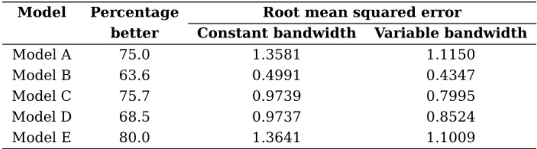
This section examines the performance of the proposed variable bandwidth selection method via several data sets of univariate regression, generated from known functions. For comparison, we also compare the performance of the constant bandwidth method, based on the direct plug-in methodology described by Ruppert et al. (1995).
As the true regression function is known in each case, the performances of the bandwidth methods are measured and compared using the root mean squared error,
RMSE
=
n
−1 nX
i=1[ ˆ
m
n(
X
i,
h
n,
α
)
−
m
(
X
i)]
2!
1/2.
and the covariate
X
has a Uniform(
−
2, 2
)
distribution. Model A:m
A(
x
) =
x
2+
x
σ
2A(
x
) =
32x
2+
0.04
Model B:m
B(
x
) = (
1
+
x
)
sin
(
1.5x
)
σ
2B(
x
) =
3.2
x
2+
0.04
Model C:m
C(
x
) =
x
+
2 exp
(
−
2
x
2)
σ
2C(
x
) =
16
(
x
2−
0.01
)
I
(x2>0.01)+
0.04
Model D:
m
D(
x
) =
sin
(
2x
) +
2 exp
(
−
2x
2)
σ
2D(
x
) =
16
(
x
2−
0.01
)
I
(x2>0.01)+
0.04
Model E:
m
E(
x
) =
exp
(
−
(
x
+
1
)
2) +
2 exp
(
−
2x
2)
σ
2E(
x
) =
32
(
x
2−
0.01
)
I
(x2>0.01)+
0.04
We draw 1000 random samples of size 200 from each model. Table 1 presents a summary of the results and shows that the variable bandwidth method has smaller RMSE than the constant bandwidth method in each case. For each model, the variable bandwidth method has smaller RMSE than the constant bandwidth method, and is better for more than 50% of samples.
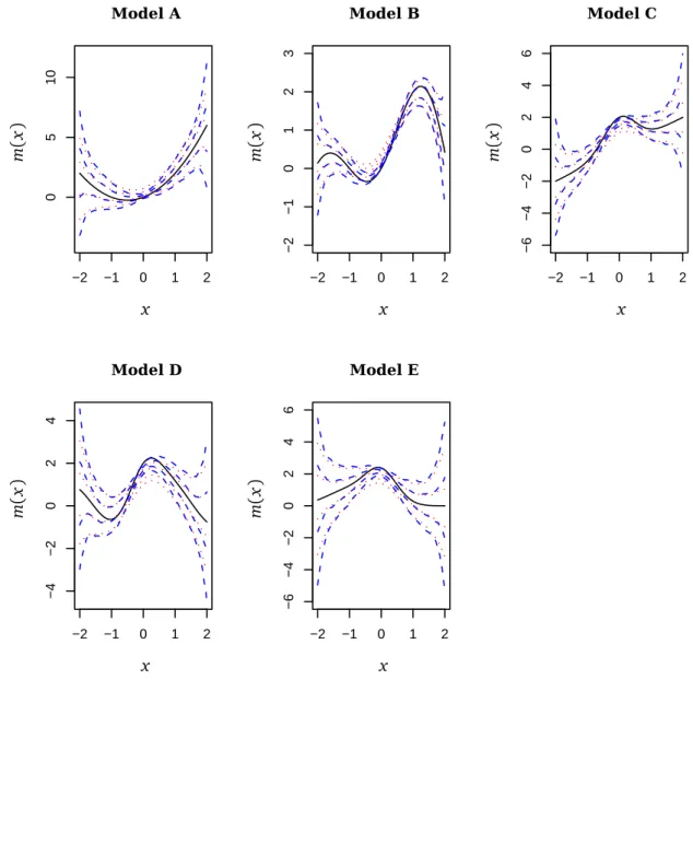
We plot the true regression functions (the solid line) and four typical estimated curves in Fig-ure 1. These correspond to the 10th, 30th, 70th and 90th percentiles. For each percentile, the variable bandwidth method (dotted line) is closer to the true regression function than the constant bandwidth method (dashed line). Therefore, we conclude that for heteroscedastic models, the local linear estimator with variable bandwidth has better goodness-of-fit than the local linear estimator with constant bandwidth.
5 Numerical studies with bivariate regression
We now examine the performance of the proposed variable bandwidth selection method via several data sets of bivariate regression, generated from known functions. For comparison, we also compare the performance of a constant bandwidth method given by
ˆ
h
=
ˆ
σ
2π
P
ni=1s
2( ˆ
H
m(
X
i))
1/6 whereˆ
σ
2=
n
−1 nX
i=1ˆ
u
2i,
and
u
i andH
ˆ
mare the same as for the variable bandwidth selector.We simulate data from four models, each with
Y
=
m
(
X
1,
X
2) +
σ
(
X
1)
u
whereu
∼
N
(
0, 1
)
andthe covariates
X
1 andX
2 are independent and have a Uniform(
−
2, 2
)
distribution.Model F:
m
A(
x
1,
x
2) =
x
1x
2σ
2A(
x
1,
x
2) = (
x
12−
0.04
)
I
(x2 1>0.04)+
0.01
Model G:m
B(
x
1,
x
2) =
x
1exp
(
−
2x
22)
σ
2B(
x
1,
x
2) =
2.5
(
x
12−
0.04
)
I
(x2 1>0.04)+
0.025
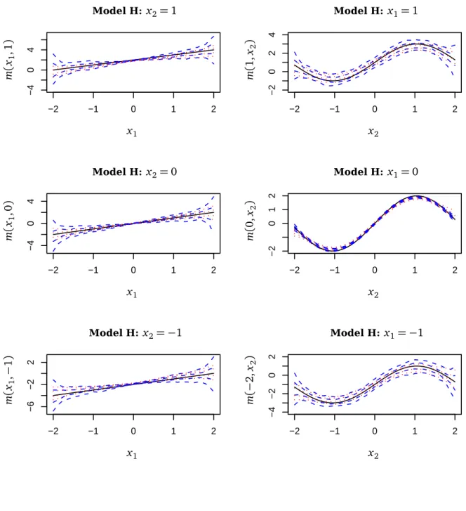
Model H:m
C(
x
1,
x
2) =
x
1+
2 sin
(
1.5x
2)
σ
2 C(
x
1,
x
2) = (
x
12−
0.04
)
I
(x2 1>0.04)+
0.01
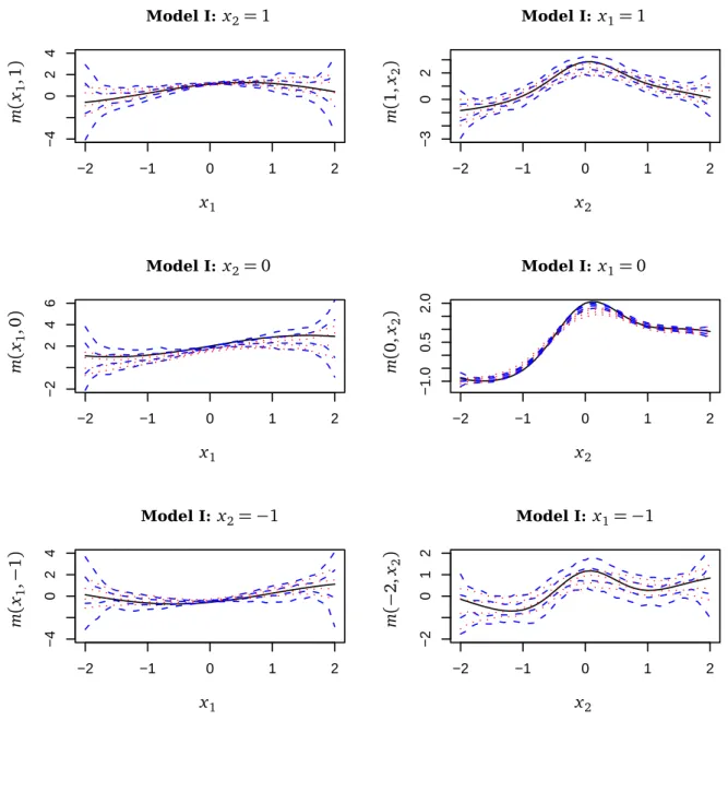
Model I:
m
D(
x
1,
x
2) =
sin
(
x
1+
x
2) +
2 exp
(
−
2x
22)
σ
2D(
x
1,
x
2) =
3
(
x
12−
0.04
)
I
(x21>0.04)
+
0.03
We draw 200 random samples of size 400 from each model.Table 2 presents a summary of the results and shows that the variable bandwidth method has smaller RMSE than the constant bandwidth method. For each model, the variable bandwidth method has lower RMSE than the constant bandwidth method and is better for more than 50% of samples.
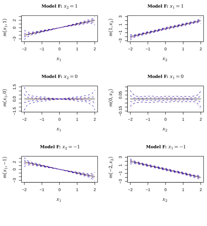
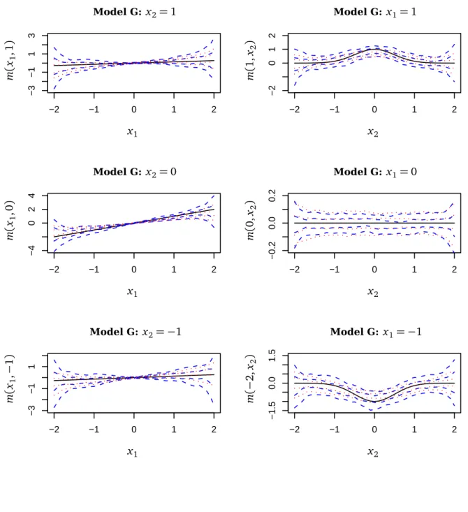
We plot the true regression functions with one fixed variable (solid line) and four typical esti-mated curves in Figures 2–5. These correspond to the 10th, 30th, 70th and 90th percentiles. For each percentile, the variable bandwidth method (dotted line) is closer to the true regression function than the constant bandwidth method (dashed line). Therefore, we conclude that for heteroscedastic models, the local linear estimator with variable bandwidth has better goodness-of-fit than the local linear estimator with constant bandwidth.
6 Summary
We have presented a local linear nonparametric estimator with variable bandwidth for multi-variate regression models. We have shown that the estimator is consistent and asymptotically normal in the interior of the sample space. We have also shown that its convergence rate is optimal for nonparametric regression (Stone, 1980, 1982).
By minimizing the conditional mean squared error of the estimator, we have derived the optimal variable bandwidth as a function of the density of the explanatory variables and the conditional variance. We have also provided a plug-in algorithm for computing the estimator when
d
=
1
ord
=
2
. Numerical simulation shows that our local linear estimator with variable bandwidth has better goodness-of-fit than the local linear estimator with constant bandwidth for heteroscedas-tic models.Acknowledgements
References
Dette, H. and A. Munk (1998) Testing heteroscedasticity in nonparametric regression, Journal
of the Royal Statistical Society, Series B,60(4), 693–708.
Efromovich, S. and M. Pinsker (1996) Sharp-optimal and adaptive estimation for heteroscedas-tic nonparametric regression,Statistica Sinica,6, 925–942.
Eubank, R. L. and W. Thomas (1993) Detecting heteroscedasticity in nonparametric regression,
Journal of the Royal Statistical Society, Series B,55(1), 145–155.
Fan, J. and I. Gijbels (1992) Variable bandwidth and local linear regression smoothers, The
Annals of Statistics,20(4), 2008–2036.
Fan, J. and I. Gijbels (1995) Data-driven bandwidth selection in local polynomial fitting: variable bandwidth and spatial adaptation, Journal of the Royal Statistical Society, Series B, 57(2), 371–394.
Fan, J. and I. Gijbels (1996)Local polynomial modelling and its applications, Chapman and Hall. Müller, H.-G. and U. Stadtmüller (1987) Variable bandwidth kernel estimators of regression
curves,The Annals of Statistics,15(1), 182–201.
Ruppert, D., S. J. Sheather and M. P. Wand (1995) An effective bandwidth selector for local least squares regression (Corr: 96V91 p1380),Journal of the American Statistical Association,90, 1257–1270.
Ruppert, D. and M. P. Wand (1994) Multivariate locally weighted least squares regression, The
Annals of Statistics,22(3), 1346–1370.
Ruppert, D., M. P. Wand, U. Holst and O. Hössjer (1997) Local polynomial variance-function estimation,Technometrics,39(3), 262–273.
Scott, D. W. (1992) Multivariate Density Estimation: Theory, Practice, and Visualization, John Wiley & Sons.
Sheather, S. J. and M. C. Jones (1991) A reliable data-based bandwidth selection method for kernel density estimation,J.R. Statist. Soc. B,53(3), 683–690.
Stone, C. J. (1980) Optimal convergence rates for nonparametric estimators, The Annals of
Statistics,8, 1348–1360.
Stone, C. J. (1982) Optimal global rates of convergence for nonparametric regression,The
An-nals of Statistics,10, 1040–1053.
Wand, M. P. and M. C. Jones (1995)Kernel Smoothing, Chapman and Hall, London. White, H. (1984)Asymptotic theory for econometricians, Academic Press.
Yatchew, A. (1998) Nonparametric regression techniques in economics, Journal of Economic
Appendix: Proof of Theorem 1
Before we state a lemma that will be used in the proof, note that
n
−1X
xTW
x,αX
x=
n
−1
P
n i=1K
hnα(Xi)(
X
i−
x
)
P
n i=1K
hnα(Xi)(
X
i−
x
)(
X
i−
x
)
TP
n i=1K
hnα(Xi)(
X
i−
x
)(
X
i−
x
)
P
n i=1K
hnα(Xi)(
X
i−
x
)(
X
i−
x
)(
X
i−
x
)
T
ande
1T(
X
xTW
x,αX
x)
−1X
xTW
x,αX
x
m
(
x
)
D
m(
x
)
=
e
T 1
m
(
x
)
D
m(
x
)
=
m
(
x
)
,
whereD
m(
x
) =
h
∂ m(x) ∂x1, . . . ,
∂m(x) ∂xdi
T . Therefore,ˆ
m
n(
x
,
h
n,
α
)
−
m
(
x
) =
e
T1(
X
xTW
x,αX
x)
−1X
xTW
x,α[
0.5
Q
m(
x
) +
U
]
,
whereQ
m(
x
) =
Q
m,1(
x
)
, . . . ,
Q
m,n(
x
)
T ,Q
m,i(
x
) = (
X
i−
x
)
TH
m(
z
i(
x
,
X
i))(
X
i−
x
)
,H
m(
x
) =
∂2m(x) ∂xi∂xj
d×d,k
z
i(
x
,
X
i)
−
x
k ≤ k
X
i−
x
k
andU
= (
u
1, . . . ,
u
n)
T. We can deduce that{
z
i(
x
,
X
i)
}
ni=1are independent because{
X
i}
ni=1 are independent.Now we state a lemma using the notation of (1) and Theorem 1.
Lemma 1 Let
G
(
α
,
f
,
x
) =
f
(
x
)
Z
supp(K)uD
αT(
x
)
uu
TD
K(
u
)
d
u
+
µ
2(
K
)
h
d f
(
x
)
D
α(
x
) +
α
−1(
x
)
D
f(
x
)
i
,
B
(
x
,
α
) =
−
µ
2(
K
)
−1f
(
x
)
−2α
(
x
)
G
(
α
,
f
,
x
)
Tand
1
be a generic matrix having each entry equal to 1, the dimensions of which will be clearfrom the context. Then
n
−1 nX
i=1K
hnα(Xi)(
X
i−
x
) =
f
(
x
) +
o
p(
1
)
(2)n
−1 nX
i=1K
hnα(Xi)(
X
i−
x
)(
X
i−
x
) =
h
2 nα
3(
x
)
G
(
α
,
f
,
x
) +
o
p(
h
2n1
)
(3)n
−1 nX
i=1K
h nα(Xi)(
X
i−
x
)(
X
i−
x
)(
X
i−
x
)
T=
µ
2(
K
)
h
2nα
2(
x
)
f
(
x
)
I
+
o
p(
h
2n1
)
(4)(
X
xTW
x,αX
x)
−1=
f
(
x
)
−1+
o
p(
1
)
B
(
x
,
α
) +
o
p(
1
)
B
T(
x
,
α
) +
o
p(
1
)
µ
2(
K
)
−1h
−n2α
−2(
x
)
f
(
x
)
−1I
+
o
p(
h
−n21
)
(5)n
−1X
xTW
x,αQ
m(
x
) =
h
2n
f
(
x
)
µ
2(
K
)
α
2(
x
)
s
(
H
m(
x
))
0
+
o
p(
h
2 n1
)
(6) and(
nh
dn)
1/2(
n
−1X
xTW
x,αu
)
d−→
N0 ,
R
(
K
)
α
−d(
x
)
σ
2(
x
)
f
(
x
)
0
(7)We only prove results (3), (6) and (7) as the other results can be proved similarly.
Proof of (3)
It is easy to show that
n
−1 nX
i=1K
hnα(Xi)(
X
i−
x
)(
X
i−
x
) =
E
K
hnα(X 1)(
X
1−
x
)(
X
1−
x
)
+
O
p(
p
n
−1Ψ
)
,
(8) whereΨ
=
Var(
K
hnα(X 1)(
X
1−
x
)(
X
11−
x
1))
, . . . ,
Var(
K
hnα(X1)(
X
1−
x
)(
X
d1−
x
d))
T .Because
x
is a fixed point in the interior of supp(
f
) =
{
x
|
f
(
x
)
6
=
0
}
, we have supp(
K
)
⊂ {
z
:
(
x
+
h
nα
(
x
)
z
)
∈
supp(
f
)
}
,
provided the bandwidth
h
n is small enough.Due to the continuity of
f
,K
andα, we have
E
K
hnα(X1)(
X
1−
x
)(
X
1−
x
)
=
Z
supp(f)h
−ndα
−d(
x
)
K
(
h
−n1(
α
(
X
1))
−1(
X
1−
x
))(
X
1−
x
)
f
(
X
1)
d
X
1=
Z
Ωn(
α
(
x
+
h
nQ
))
−dK
(
Q
(
α
(
x
+
h
nQ
))
−1)
f
(
x
+
h
nQ
)
h
nQ
d
Q
=
h
2nα
(
x
)
3G
(
α
,
f
,
x
) +
o
(
h
2n1
)
,
(9) whereΩ
n=
{
Q
:
x
+
h
nQ
∈
supp(
f
)
}
. It is easy to see Var
K
h nα(X1)(
X
1−
x
)(
X
1−
x
)
=
En
K
h nα(X1)(
X
1−
x
)(
X
1−
x
)
K
h nα(X1)(
X
1−
x
)(
X
1−
x
)
To
−
¦
E
K
h nα(X1)(
X
1−
x
)(
X
1−
x
)
© ¦
E
K
h nα(X1)(
X
1−
x
)(
X
1−
x
)
©
T.
(10)Again by the continuity of
f
,K
andα, we have
E
n
K
hnα(X1)(
X
1−
x
)(
X
1−
x
)
K
hnα(X1)(
X
1−
x
)(
X
1−
x
)
To
=
E
K
hnα(X1)(
X
1−
x
)
2(
X
1−
x
)(
X
1−
x
)
T
=
Z
supp(f)
h
−nd(
α
(
x
))
−dK
(
h
−n1(
α
(
X
1))
−1(
X
1−
x
))
2(
X
1−
x
)(
X
1−
x
)
Tf
(
X
1)
d
X
1=
h
−nd+2Z
Ωn(
α
(
x
+
h
nQ
))
−dK
(
Q
(
α
(
x
+
h
nQ
))
−1)
2f
(
x
+
h
nQ
)
d
Q
=
h
−nd+2Z
Ωn(
α
(
x
))
−dK
(
Q
(
α
(
x
))
−1)
2f
(
x
)
d
Q
+
O
(
h
−nd+21
) =
O
(
h
−d+2 n1
)
.
(11) Therefore we haveO
p(
p
n
−1Ψ
) =
o
p(
h
2n1
)
.
(12)Then (3) follows from (8)–(12).
Proof of (6)
It is straightforward to show that
=
n
−1P
ni=1K
hnα(Xi)(
X
i−
x
)(
X
i−
x
)
TH
m(
z
i(
x
,
X
i))(
X
i−
x
)
n
−1P
ni=1K
hnα(Xi)(
X
i−
x
)(
X
i−
x
)
TH
m(
z
i(
x
,
X
i))(
X
i−
x
)(
X
i−
x
)
,
n
−1 nX
i=1K
hnα(Xi)(
X
i−
x
)(
X
i−
x
)
TH
m(
z
i(
x
,
X
i))(
X
i−
x
)
=
h
2nf
(
x
)
µ
2(
K
)(
α
(
x
))
2s
(
H
m(
x
)) +
o
p(
h
2n1
)
,
andn
−1 nX
i=1K
h nα(Xi)(
X
i−
x
)(
X
i−
x
)
TH
m(
z
i(
x
,
X
i))(
X
i−
x
)(
X
i−
x
) =
O
p(
h
3n1
)
.
Therefore (6) holds. Proof of (7) It is obvious that En
−1X
xTW
x,αu
=
En
−1X
xTW
x,αu
|
x
=
0
,
andn
−1X
xTW
x,αu
=
n
−1P
ni=1K
h nα(Xi)(
X
i−
x
)
u
in
−1P
ni=1K
hnα(Xi)(
X
i−
x
)(
X
i−
x
)
u
i
.
By the continuity of
f
,K
,σ
2andα, we have
Var
n
−1 nX
i=1K
h nα(Xi)(
X
i−
x
)
u
i
=
n
−1Var
K
h nα(X1)(
X
1−
x
)
u
1
=
n
−1Z
supp(f)
h
−nd(
α
(
x
))
−dK
(
h
−n1(
α
(
X
1))
−1(
X
1−
x
))
2σ
2(
X
1)
f
(
X
1)
d
X
1=
n
−1h
−ndZ
Ωn((
α
(
x
+
h
nQ
))
−dK
(
Q
(
α
(
x
+
h
nQ
))
−1))
2σ
2(
x
+
h
nQ
)
f
(
x
+
h
nQ
)
d
Q
=
n
−1h
−ndZ
Ωn((
α
(
x
))
−dK
(
Q
(
α
(
x
))
−1))
2σ
2(
x
)
f
(
x
)
d
Q
+
o
(
n
−1h
−d n)
=
n
−1h
−ndR
(
K
)(
α
(
x
))
−dσ
2(
x
)
f
(
x
) +
o
(
n
−1h
−nd)
,
and Var
n
−1 nX
i=1K
hnα(Xi)(
X
i−
x
)(
X
i−
x
)
u
i
=
o
(
n
−1h
−nd+21
)
. Then (7) holds.Proof of Theorem 1
By (5) and (6), we have
E
[ ˆ
m
n(
x
,
h
n,
α
)
|
X
1, . . . ,
X
n]
−
m
(
x
) =
0.5
e
T1(
X
xTW
x,αX
x)
−1X
xTW
x,αQ
m(
x
)
=
0.5h
2nµ
2(
K
)(
α
(
x
))
2s
(
H
m(
x
)) +
o
p(
h
2n)
.
Therefore Theorem 1(1) holds.
Let
V
=
diagσ
2(
X
1)
, . . . ,
σ
2(
X
n)
. ThenVar
[ ˆ
m
n(
x
,
h
n,
α
)
|
X
1, . . . ,
X
n] =
e
T1(
X
xTW
x,αX
x)
−1X
xTW
x,αV W
x,αX
x(
X
xTW
x,αX
x)
−1e
1,
(13) andn
−1X
xTW
x,αV W
x,αX
x=
a
11(
x
,
h
n,
α
)
(
a
21(
x
,
h
n,
α
))
Ta
21(
x
,
h
n,
α
)
a
22(
x
,
h
n,
α
)
,
wherea
11(
x
,
h
n,
α
) =
n
−1 nX
i=1(
K
hnα(Xi)(
X
i−
x
))
2σ
2(
X
i)
a
21(
x
,
h
n,
α
) =
n
−1 nX
i=1(
K
h nα(Xi)(
X
i−
x
))
2(
X
i−
x
)
σ
2(
X
i)
anda
22(
x
,
h
n,
α
) =
n
−1 nX
i=1(
K
hnα(Xi)(
X
i−
x
))
2(
X
i−
x
)(
X
i−
x
)
Tσ
2(
X
i)
.
It is easy to prove that
n
−1 nX
i=1(
K
hnα(Xi)(
X
i−
x
))
2σ
2(
X
i) =
h
−ndR
(
K
)(
α
(
x
))
−dσ
2(
x
)
f
(
x
)
o
p(
h
−nd)
,
n
−1 nX
i=1(
K
h nα(Xi)(
X
i−
x
))
2(
X
i−
x
)
Tσ
2(
X
i) =
O
p(
h
−nd+11
)
andn
−1 nX
i=1(
K
hnα(Xi)(
X
i−
x
))
2(
X
i−
x
)(
X
i−
x
)
Tσ
2(
X
i) =
O
p(
h
−nd+21
)
.
(14) By (13)–(14) and (5), we have Var[ ˆ
m
n(
x
,
h
n,
α
)
|
X
1, . . . ,
X
n] =
n
−1h
−ndR
(
K
)(
α
(
x
))
−dσ
2(
x
)
f
(
x
)
−1+
o
p(
n
−1h
−nd)
.
Therefore Theorem 1(2) holds.
By (6) and (7) and the central limit theorem, we have
n
2/(d+4)n
−1X
xTW
x,α[
0.5
Q
m(
x
) +
u
]
d−→
N
(
0.5c
2µ
2(
K
)(
α
(
x
))
2f
(
x
)
s
(
H
m(
x
))
,
c
−dR
(
K
)(
α
(
x
))
−dσ
2(
x
)
f
(
x
))
0
.
Tables
Table 1: The percentage of 1000 samples in which the variable bandwidth method is better
than the constant bandwidth method, and the RMSE of the two methods.
Model Percentage Root mean squared error
better Constant bandwidth Variable bandwidth
Model A 75.0 1.3581 1.1150
Model B 63.6 0.4991 0.4347
Model C 75.7 0.9739 0.7995
Model D 68.5 0.9737 0.8524
Model E 80.0 1.3641 1.1009
Table 2: The percentage of 200 samples in which the variable bandwidth method is better than
the constant bandwidth method, and the RMSE of the two methods.
Model Percentage Root mean squared error
better Constant bandwidth Variable bandwidth
Model F 54.6 0.0411 0.0397
Model G 54.0 0.0843 0.0816
Model H 53.0 0.0935 0.0814
Figures
Figure 1: Results for the simulated univariate regression data of models A–E. The true
regres-sion functions (the solid line) and four typical estimated curves are presented. These corre-spond to the 10th, the 30th, the 70th, the 90th percentile. The dashed line is for the constant bandwidth method and the dotted line is for the variable bandwidth method.
−2 −1 0 1 2 0 5 10 −2 −1 0 1 2 −2 −1 0 1 2 3 −2 −1 0 1 2 −6 −4 −2 0 2 4 6 −2 −1 0 1 2 −4 −2 0 2 4 −2 −1 0 1 2 −6 −4 −2 0 2 4 6
x
x
x
x
x
m
(
x
)
m
(
x
)
m
(
x
)
m
(
x
)
m
(
x
)
Model A Model B Model C
Figure 2: Results for the simulated bivariate data of model F. The true regression functions (the solid line) and four typical estimated curves are presented. These correspond to the 10th, the 30th, the 70th, the 90th percentile. The dashed line is for the constant bandwidth method and the dotted line is for the variable bandwidth method.
−2 −1 0 1 2 −3 0 2 −2 −1 0 1 2 −3 −1 1 3 −2 −1 0 1 2 −1.5 0.0 1.5 −2 −1 0 1 2 −0.15 0.05 −2 −1 0 1 2 −3 0 2 −2 −1 0 1 2 −3 −1 1 3
m
(
x
1,0
)
m
(
x
1,1
)
m
(
x
1,
−
1
)
m
(
−
2
,
x
2)
m
(
0
,
x
2)
m
(
1
,
x
2)
x
1x
1x
1x
2x
2x
2 Model F:x
1=
1
Model F:x
1=
0
Model F:x
1=
−
1
Model F:x
2=
1
Model F:x
2=
0
Model F:x
2=
−
1
Figure 3: Results for the simulated bivariate data of model G. The true regression functions (the solid line) and four typical estimated curves are presented. These correspond to the 10th, the 30th, the 70th, the 90th percentile. The dashed line is for the constant bandwidth method and the dotted line is for the variable bandwidth method.
−2 −1 0 1 2 −3 −1 1 3 −2 −1 0 1 2 −2 0 1 2 −2 −1 0 1 2 −4 0 2 4 −2 −1 0 1 2 −0.2 0.0 0.2 −2 −1 0 1 2 −3 −1 1 −2 −1 0 1 2 −1.5 0.0 1.5
m
(
x
1,0
)
m
(
x
1,1
)
m
(
x
1,
−
1
)
m
(
−
2
,
x
2)
m
(
0
,
x
2)
m
(
1
,
x
2)
x
1x
1x
1x
2x
2x
2 Model G:x
1=
1
Model G:x
1=
0
Model G:x
1=
−
1
Model G:x
2=
1
Model G:x
2=
0
Model G:x
2=
−
1
Figure 4: Results for the simulated bivariate data of model H. The true regression functions (the solid line) and four typical estimated curves are presented. These correspond to the 10th, the 30th, the 70th, the 90th percentile. The dashed line is for the constant bandwidth method and the dotted line is for the variable bandwidth method.
−2 −1 0 1 2 −4 0 4 −2 −1 0 1 2 −2 0 2 4 −2 −1 0 1 2 −4 0 4 −2 −1 0 1 2 −2 0 1 2 −2 −1 0 1 2 −6 −2 2 −2 −1 0 1 2 −4 −2 0 2
m
(
x
1,0
)
m
(
x
1,1
)
m
(
x
1,
−
1
)
m
(
−
2
,
x
2)
m
(
0
,
x
2)
m
(
1
,
x
2)
x
1x
1x
1x
2x
2x
2 Model H:x
1=
1
Model H:x
1=
0
Model H:x
1=
−
1
Model H:x
2=
1
Model H:x
2=
0
Model H:x
2=
−
1
Figure 5: Results for the simulated bivariate data of model I. The true regression functions (the solid line) and four typical estimated curves are presented. These correspond to the 10th, the 30th, the 70th, the 90th percentile. The dashed line is for the constant bandwidth method and the dotted line is for the variable bandwidth method.
−2 −1 0 1 2 −4 0 2 4 −2 −1 0 1 2 −3 0 2 −2 −1 0 1 2 −2 2 4 6 −2 −1 0 1 2 −1.0 0.5 2.0 −2 −1 0 1 2 −4 0 2 4 −2 −1 0 1 2 −2 0 1 2