Real-Time Implementation of an ISM Fault Tolerant
Control Scheme for LPV Plants
H. Alwi, C. Edwards, O. Stroosma, J. A. Mulder and M. T. Hamayun
Abstract
This paper proposes a fault tolerant control scheme for linear parameter varying systems based on integral sliding modes and control allocation, and describes the implementation and evaluation of the controllers on a 6 degree-of-freedom research flight simulator called SIMONA. The fault tolerant control scheme is developed using a linear parameter varying approach to extend ideas previously developed for linear time invariant systems, in order to cover a wide range of operating conditions. The scheme benefits from the combination of the inherent robustness properties of integral sliding modes (to ensure sliding occurs throughout the simulation) and control allocation, which has the ability to redistribute control signals to all available actuators in the event of faults/failures.
Index Terms
Sliding mode control, Fault tolerance, Aerospace simulation.
I. INTRODUCTION
The most important facet of Fault Tolerant Control (FTC) systems is their ability to maintain closed-loop stability, and ideally a measure of performance, in the face of faults or failures in actuators or sensors. The majority of the FTC methods that have appeared in the literature are based on linear time invariant (LTI) systems (see for example [1]). There are however notable exceptions: for example an observer based scheme for a specific class of input-output stable nonlinear systems is proposed in [2]; a passive FTC approach is proposed in [3] for a class of affine nonlinear systems considering actuator faults; and in [4], a FTC scheme for a specific class of nonlinear systems is proposed based on a sliding mode control allocation scheme incorporating a backstepping controller.
Linear parameter varying (LPV) systems are a special class of finite dimensional linear systems, in which the entries of the state space matrices continuously depend on a time varying parameter vector which belongs to a bounded compact set. Using LPV techniques, the control law can be automatically ‘scheduled’ with the operating conditions and guaranteed performance can be proved over a wide operating envelope. FDI and FTC methods designed for LPV models have appeared in the literature. In [5], a synthesis method using LMIs is presented in order to guarantee closed-loop stability in the case of multiple actuator faults. In [6] an FDI scheme based on the extension of residual generation concepts for LTI systems was presented and tested on a model of a B747-100/200.
Sliding mode control (SMC) is attractive from an FTC stand point, since actuator faults can be modelled as matched uncertainty, which is precisely the class of uncertainty to which sliding modes are robust [7]. However SMC cannot directly deal with total actuator failures because the complete loss of effectiveness in a channel destroys the regularity of the sliding mode, and an unique equivalent control signal can no longer be determined. To obviate this short-coming, in over actuated systems, a combination of SMC and control allocation (CA) has recently been explored [8]. In this context, CA can be viewed as a mechanism for distributing a virtual control signal to specific actuator commands to effect fault tolerant control. In
H. Alwi and C. Edwards are with the College of Engineering, Mathematics and Physical Sciences, University of Exeter, EX4 4QF, UK. [email protected], [email protected]
O. Stroosma and J. A. Mulder are with the Control and Simulation section of the Faculty of Aerospace Engineering, Delft University of Technology, Kluyverweg 1, 2629HS, The Netherlands. [email protected], [email protected]
M.T. Hamayun is with COMSATS, M.A Jinnah Building, COMSATS Lahore campus, Pakistan. [email protected]
This preprint have been accepted for publication in the IEEE Transactions On Industrial Electronics, 2015 (DOI: 10.1109/TIE.2014.2386279)
the earliest work [8] first order sliding mode concepts were considered. More recently, in [9], integral sliding mode (ISM) ideas have been combined with CA. However all the SMC/CA and ISM/CA methods cited above are based on LTI system descriptions of the plant to be controlled and are restricted to near trim conditions.
One of the main contributions of this paper is to extend the previous work in [8] in order to create an integral sliding mode control allocation scheme for LPV systems having affine parameter dependence. There is very little literature on the use of sliding mode controllers for LPV systems with the notable exception of [10] and more recently [11]. The work in [10] proposed SMC schemes for LPV systems (although not in the context of fault tolerant control). In the proposed scheme, it is assumed that (fault-free) full state information is available for controller design, together with estimates of the actuator health levels. The proposed scheme takes into account imperfect estimation of the actuator health levels by using an adaptive scalar modulation function in the nonlinear part of the (virtual) control law. This is different to the adaptation scheme considered in [7] which considers a LTI based design problem. The virtual control law designed by the ISM technique is then translated into actual actuator commands using the CA scheme. The resulting FTC scheme guarantees closed-loop stability and performance in the presence of a class of total actuator failures over a wide part of the flight envelope.
Another contribution of this paper is the implementation and evaluation of the proposed scheme on the 6 degree-of-freedom research simulator called SIMONA, (Simulation Motion and Navigation) [12]. This has been carried out not only to demonstrate the efficacy of the proposed adaptive LPV FTC scheme, but also to show the potential of the proposed scheme for industrial usage. There is work in the literature describing the implementation of SMC FTC schemes on a flight simulator, however most involve designs based on LTI systems which are theoretically only valid near the trim condition. The results in this paper represent the only published implementations of an ISM FTC scheme on a flight simulator.
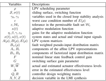
The notation used in this paper is standard: IR represents the real numbers whilst IRn×m denotes an n by m matrix with elements in IR. For a vector, ∥ · ∥ represents the Euclidean norm, and the induced spectral norm for matrices. The important variables are given in Table I.
TABLE I IMPORTANT VARIABLES
Variables Descriptions
ρ LPV scheduling parameter
S, σ(t) sliding surface, switching function
γ0, γ1 variables used in the closed loop stability analysis
c worst case condition number ofE(ρ)
ε,Wε tolerance in the permissable fault setWε
κ(t) adaptive modulation function
η, β, γ, ε0 gains for the adaptive modulation function
x(t), u(t), ν(t) system states and actual and virtual input signals A(ρ), B(ρ), E(ρ) LPV system matrices
Bw(ρ) fault weighted pseudo-input distribution matrix
Ai, Bi components of the affine LPV representations
B1, B2 components of factorized input distribution matrix
F nominal linear state feedback control gain
G switching surface gain parameter
W,cW actual and estimated actuator effectiveness levels
∆ error in the estimated effectiveness level Q, R controller design weighting matrix
X, Y, Z decision variable in the LMI synthesis
II. PROBLEMFORMULATION Consider a LPV plant subject to actuator faults/failures
˙
where the system and input matrices A(ρ)∈IRn×n, B(ρ)∈IRn×m and vary with respect to a scheduling parameter ρ(t) ∈ IRr. In this paper all the states are assumed to be available for control purposes. The diagonal semi-positive definite matrix W(t) ∈ IRm×m with diagonal entries w1(t), . . . wm(t) model the effectiveness levels of the actuators. If wi(t) = 1then the ith actuator is working perfectly (i.e. fault-free), whereas if1> wi(t)>0a partial fault is present and the actuator works at reduced efficiency. Ifwi(t) = 0 then the ith actuator has completely failed and the control signal component u
i(t) has no effect on the system. The time varying parameter vector ρ(t)∈IRr is also assumed to be available and furthermore is assumed to lie in a bounded compact set Ω⊂IRr. Also it is assumed that matrix A(ρ) depends affinely on ρ(t) so that
A(ρ) =A0+
∑r i=1Aiρi for some Ai ∈IRn×n and that B(ρ) can be factorized as
B(ρ) =BfE(ρ) (2)
whereBf ∈IRn×m is a fixed matrix and E(ρ)∈IRm×m is a matrix depending explicitly on the scheduling variable ρ(t). Furthermore assume E(ρ) is invertible for all ρ(t)∈Ω.
Assume that, by permuting the states (if necessary), the matrix Bf in (2) can be expressed as Bf = [ B1 B2 ] (3) with B1 ∈ IR(n−l)×m and B2 ∈ IRl×m where B2 is of rank l < m. In this paper it is assumed that
∥B2∥ ≫ ∥B1∥so that theB2 represents the dominant contribution of the distribution of the control action
within the channels of the system [8].
Finally without loss of generality, scale the last l states of the system to ensure that B2B2T = Il. This simplifies some of the subsequent algebra and will be exploited in several places in the ensuing analysis. Consider a ‘virtual control’ signal
ν(t) := B2E(ρ)u(t) (4)
The signal ν(t)∈IRl can be viewed as the total control effort produced by the actuators. Exploiting the fact B2B2T =Il, one choice for the physical control law u(t)∈IRm is
u(t) := (E(ρ))−1B2Tν(t) (5)
Note the expression foru(t)in equation (5) above satisfies (4) since(E(ρ))−1BT
2 is a right pseudo inverse of B2E(ρ).
Remark: The control structure proposed in (5) is different from [9], [8], since it involves the varying matrixE(ρ)and the control allocation scheme does not require any knowledge of the actuator effectiveness level W(t).
Using (1),(3) and substituting for u(t) from (5) yields the state space representation
˙ x(t) = A(ρ)x(t) + [ B1E(ρ)W(t)(E(ρ))−1B2T B2E(ρ)W(t)(E(ρ))−1B2T ] | {z } Bw(ρ) ν(t) (6)
in terms of the virtual controlν(t). Note that, when the system is fault-free, i.e. whenW(t) = I, exploiting the fact that B2BT2 =Il, equation (6) simplifies to
˙ x(t) =A(ρ)x(t) + [ B1BT2 Il ] | {z } Bν ν(t) (7)
Assume there exists a symmetric positive definite matrix P ∈IRn×n and a matrix F ∈IRm×n, depending on the scheduling variable, such that
(A(ρ)−BνF)TP +P(A(ρ)−BνF)<0 (8)
for all admissibleρ(t)∈Ω. In other words, there exists a state feedback virtual control lawν(t) = −F x(t)
such that
˙
x(t) = (A(ρ)−BνF)x(t) (9)
is quadratically stable for all ρ(t)∈Ω and achieves the desired closed-loop performance. III. INTEGRAL SLIDING MODE CONTROLLER DESIGN
A. Design of Integral switching function:
In this section Integral sliding mode ideas [13], [9] will be used to create a fault tolerant control scheme. One advantage of ISM schemes over traditional sliding modes is they eliminate the ‘reaching phase’ associated with traditional sliding mode control. Consider the (integral) sliding surface
S ={x∈IRn : σ(t) = 0} where σ(t) :=Gx(t)−Gx(0)−G ∫ t 0 (A(ρ)−BνF)x(τ)dτ (10)
The design freedom in (10) is represented by the fixed matrix G ∈ IRl×n. In this paper, the particular choice of
G:=B2(BfTBf)−1BfT (11)
is made, where B2 and Bf are defined in (2) and (3). Based on the choice of G in (11), and exploiting the fact that B2BT2 =Il, it can be verified that
GBν =B2(BfTBf)−1BfTBfB2T =Il (12)
Furthermore
GBw(ρ) = B2(BfTBf)−1BfTBfE(ρ)W(t)(E(ρ))−1B2T
= B2E(ρ)W(t)(E(ρ))−1B2T (13)
Taking the derivative of σ along the trajectories of (6) yields
˙
σ(t) = GBw(ρ)ν(t) +GBνF x(t) =GBw(ρ)ν(t) +F x(t) (14) after substituting from (6) and (12). Arguing as in [9] the sliding motion is governed by
˙ x(t) = ( A(ρ)−Bw(ρ)(B2E(ρ)W(E(ρ))−1B2T)−1F ) x(t) (15)
Note that from equation (15), for an unique equivalent control to exist and an unambiguous sliding motion to occur, det(B2E(ρ)W(t)(E(ρ))−1B2T) ̸= 0. This imposes a constraint on the allowable faults/failures W(t). Adding and subtracting BνF x(t) to the right hand side of (15), after some manipulation, the dynamics in (15) can be written as
˙ x(t) = (A(ρ)−BνF)x(t) +BeΓ(t)F x(t) (16) where Γ(t) :=B1B2T − B1E(ρ)W(t)(E(ρ))−1B2T×(B2E(ρ)W(t)(E(ρ))−1B2T)− 1 (17) and e BT :=[ In−l 0 ] (18)
Consider as the class of permissable faults/failures, those which belong to the set
Wε ={(w1, ..., wm)∈ I : (GBw(ρ))T(GBw(ρ))> εI} (19) whereI = [0 1]×...×[0 1]andεis a small scalar satisfying0< ε≪1. Note that(GBw(ρ))T(GBw(ρ))|W(t)=I = I > εI and therefore the set Wε is not empty. Furthermore, for all W = diag(w1, ..., wm) ∈ Wε, it is straightforward to show
∥(GBw(ρ))−1∥=∥(B2E(ρ)W(E(ρ))−1B2T)−
1∥< √1 ε From (17), for W ∈ Wε, using simple bounding arguments,
∥Γ(t)∥ ≤γ1(1 +
c √
ε) (20)
where by definition c= maxρ∈Ω∥E(ρ)∥∥(E(ρ))−1∥ and γ1 =∥B1∥ (which by assumption is small). The quantity c represents the worst case condition number of E(ρ).
Remark: Notice that the conditions (19)-(20) in this paper are subtly different to those for LTI systems discussed in [8], [9]. In this paper, the norm of (GBw(ρ))−1 must be guaranteed to be bounded. Here, this is achieved by limiting W(t) ∈ Wε thus introducing an explicit ε > 0 to bound ∥GBw(ρ)∥ away from zero1. This assumption is not necessary for the LTI systems considered in [8], [9] and therefore the
conditions in (19) and (20) are slightly more restrictive compared to [8], [9], in the sense that the set of the faults that can be tolerated by the controller is reduced. However the LPV models considered here will represent the underlying real plant over a wider operating regime.
B. Closed-loop stability analysis:
In a fault-free scenario when W(t) = I, it is easy to check that Γ(t) = 0 and (16) simplifies to (9) which is quadratically stable by design. However closed-loop stability of (16) needs to be proven in the case where W(t)̸=I but belongs to Wε in (19). For analysis, equation (16) can be represented by
˙ x(t) = (|A(ρ){z−BνF)} e A(ρ) x(t) +Be e u(t) z }| { Γ(t)F x(t) | {z } e y(t) (21)
Define the positive scalar γ0 to be the L2 gain associated with the operator
e
G(s) :=F(sI−Ae(ρ))−1Be (22)
Proposition 1: For any fault or failure scenarios belonging to the set Wε given in (19), the sliding motion
in (21) will be stable if
γ0γ1(1 + c √
ε)<1 (23)
Proof: The system in (21) can be regarded as the feedback interconnection of the LPV plant in (22) and
the varying feedback gain ue(t) = Γ(t)ye(t). If inequality (23) is satisfied, then from the small gain theorem [14], the system in (21) will be stable.
1
C. ISM Control Laws:
The proposed integral sliding mode control law is
ν(t) = (GBwˆ(ρ))−1(νl(t) +νn(t)) (24)
where
GBwˆ(ρ) = B2E(ρ)Wc(t)(E(ρ))−1B2T (25) and Wc(t) is an estimate of W(t). The linear part of the control law νl(t) in (24) is defined as
νl(t) :=−F x(t) (26)
and the nonlinear discontinuous part, which induces sliding and provides robustness is given by νn(t) :=−κ(t)
σ(t)
∥σ(t)∥ for σ(t)̸= 0 (27)
where κ(t)>0 is an adaptive modulation function given by
κ(t) = ∥F∥∥x(t)∥κ¯(t) +η (28)
and η is a positive scalar. The positive adaptation gain κ¯(t) evolves according to
˙¯
κ(t) = −β¯κ(t) +γε0∥F∥∥x(t)∥∥σ(t)∥ (29) where β, γ and ε0 are positive (design) scalar gains.
In the analysis which follows, it is assumed the actuator efficiency level W(t) is not perfectly known but that the estimate Wc(t) satisfies
W(t) =Wc(t)(I+ ∆(t)) (30)
where the diagonal matrix ∆(t)represents imperfections in the estimation of W(t). Substituting (30) into (13) yields
GBw(ρ) = B2E(ρ)Wc(t)(E(ρ))−1B2T+B2E(ρ)Wc(t)∆(t)(E(ρ))−1B2T (31) Using (24), equation (14) becomes
˙
σ(t) =GBw(ρ)(GBwˆ(ρ))−1(νl(t) +νn(t)) +F x(t) Substituting for (31) and for νl from (26) yields
˙ σ(t) = (I+∆(b t))(νl(t) +νn(t)) +F x(t) = (I+∆(b t))νn(t)−∆(b t)F x(t) (32) where b ∆(t) := (B2E(ρ)Wc 1 2(t)∆(t)Wc 1 2(t)(E(ρ))−1BT 2 ) ×(B2E(ρ)Wc(t)(E(ρ))−1B2T )−1 (33) Define Dε0 = { ∆(t) from (30) : ∥∆(b t)∥<√1−2ε0 } (34) for some scalar 0 < ε0 ≪ 1/2. Clearly the set Dε0 is not empty since ∆(t) = 0 ∈ Dε0. It is easy to
show that if ∥∆(b t)∥<√1−2ε0 then2Il+∆(b t) +∆bT(t)>2ε0Il. Consider the positive definite candidate Lyapunov function V(t) =σT(t)σ(t) + 1 γe 2(t) where e(t) = ¯κ(t)− 1 ε0 (35)
Since ∥∆(b t)∥<√1−2ε0, taking the derivative of σT(t)σ(t) and then substituting from (32), yields d dt(σ Tσ) = −κ(t) σT ∥σ∥ ( 2Il+∆(b t) +∆bT(t) ) σ−2σT∆(b t)F x(t) ≤ −2κ(t)ε0∥σ∥+ 2∥σ∥∥∆(b t)∥∥F x(t)∥ ≤ −2κ(t)ε0∥σ∥+ 2∥σ∥ √ 1−2ε0∥F∥ ∥x(t)∥ (36)
From (35) it follows that κ¯(t) =e(t) + ε1
0. Then using the fact that
√ 1−2ε0 <1 and substituting (28) into (36), it follows d dt(σ T(t)σ(t)) = −2ε 0∥F∥∥x(t)∥∥σ(t)∥e(t)−2ηε0∥σ(t)∥ (37) Taking the derivative of γ1e2(t), and then using the fact that e˙(t) = ˙¯κ(t), from (35)
d dt ( 1 γe 2(t) ) = −2β γ e(t)¯κ+ 2ε0e(t)∥F∥∥x(t)∥∥σ(t)∥ (38) Therefore, from (37)-(38) and substituting for κ¯(t) from (35)
˙ V(t) ≤ −2β γ e(t)¯κ−2ηε0∥σ(t)∥ = −2β γε0 e(t)− 2β γ e 2(t)−2ηε 0∥σ(t)∥ (39)
It is easy to show that
−2β γε0 e(t)− 2β γ e 2(t)≤ β 2γε2 0 for all values of e(t) and therefore from (39) it follows that
˙
V(t) ≤ β 2γε2
0
−2ηε0∥σ(t)∥ (40)
which implies that σ(t) moves into a boundary layer about σ(t) = 0 of size 4γεβ3 0η
.
Remark: The adaptation scheme in (28)-(29) makes the approach in this paper quite different from [9]. Adaptation is required here because of the complex relationship between ∆(t) and ∆(b t) in (33) and the limitations associated with (34).
Remark:The fact that a traditional sliding mode scheme involving a unit vector structure has been selected as the basis for the control law, has facilitated the inclusion of an adaptive scheme. An adaptive gain is highly desirable in FTC schemes to compensate for sudden significant changes to the plant. Although the use of a higher order sliding mode controller would be advantageous in terms of ensuring a smoother control signal (e.g. [15], [16], [17]), work describing the coupling of such schemes with adaptive gains is less mature.
Finally the physical control law which is used to distribute the control effort among the available actuators is obtained by substituting (24)-(27) into (5) which yields
u(t) = −(E(ρ))−1B2T(B2E(ρ)Wc(t)(E(ρ))−1B2T)− 1× ( F x(t) +κ(t) σ(t) ∥σ(t)∥ ) for σ(t)̸= 0 (41) Note the physical control law in (41) requires an estimate of the effectiveness level of the actuators Wc(t)
F
x
(
t
)
Plant
Actuator
ISMC
CA
FDI
u
(
t
)
c
W
(
t
)
Baseline Controller
Adaptive
W
(
t
)
u
a(
t
)
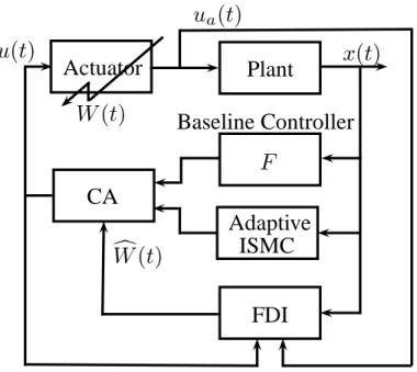
Fig. 1. Overall FTC scheme
D. Design of the state feedback gain
In designing F two objectives must be met: the first equates to achieving the required nominal performance (when W = I) for all the admissible values of ρ; and the second is associated with the closed-loop stability i.e. ensuring the small gain condition in (23) is satisfied. Nominal performance will be achieved by the use of a LQR type cost function
J =
∫ ∞
0
(xTQx+uTRu)dt (42)
whereQandR are s.p.d matrices specified by the designer. The LPV system matrices (Ae(ρ),B, Fe ) in (22) can be represented by the polytopic system (Ae(ωi),B, Fe ), where the vertices ω1, ω2, ...ωnω for nω = 2
r correspond to the extremes of the allowable range of ρ∈Ω [18], [19]. Specifically
e
A(ρ) =∑2i=1r Aeiδi,
∑2r
i=1δi = 1, δi ≥0
The minimization of J can be posed as an optimization problem: Minimize trace(X−1) subject to
[ ˇ A(ωi) ( ˜QX −RY˜ )T ˜ QX −RY˜ −I ] < 0 (43) X > 0 (44) where Aˇ(ωi) = A(ωi)X+XAT(ωi)−BνY −YTBνT, Q˜ = [(Q1/2)T 0Tl×n], R˜= [0Tl×n (R1/2)T], Y :=F X and X∈IRn×n is the Lyapunov matrix. To satisfy the stability condition in (23), it is sufficient to apply the Bounded Real Lemma at each vertex of the polytope: specifically
A(ωi)X+XAT(ωi)−BνY −YTBνT B˜ YT ˜ BT −γ2I 0 Y 0 −I <0 (45)
These conditions can be converted into an LMI problem: Minimize trace(Z) subject to
[
−Z In
In −X
]
together with (43), (44) and (45). The decision variables are Z, X and Y, and the matrix Z satisfies trace(Z)≥trace(X−1). The LMIs in (43)-(46) can be solved for all the vertices of the polytopic system [18], [19]. Finally the gains F can be recovered using the relationship F =Y X−1.
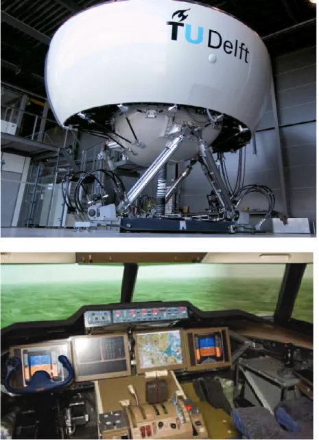
IV. RECOVERAND THESIMONA SIMULATOR
The SIMONA research simulator (SRS) (Figure 2) is a 6 degree-of-freedom motion simulator located at Delft University of Technology. The SRS can accommodate two pilots in the cockpit in a side by side arrangement. The pilot controls include a typical wheel, column and rudder pedal and side-stick configuration. There is also a thrust lever, the digital instrument panel and a mode control panel (MCP) (which has the capability to provide command signals to the ‘auto-pilot’). The visual system of the SRS coupled with the motion system, provided by six large hydraulic cylinders, provides a realistic sense of motion inside the cockpit.
(b) Cockpit view
Fig. 2. SIMONA research simulatorIn this paper, the SRS has been configured to represent a B747-100/200 large transport aircraft, based on the high fidelity nonlinear aircraft model used in the FTC benchmark RECOVER (REconfigurable COntrol for Vehicle Emergency Return) [12]. The RECOVER model consists of 77 states and includes, four engines and 25 other control surfaces (4 elevators, one stabilizer, 4 ailerons, 12 spoilers and flaps).
V. DESIGN ANDSRS IMPLEMENTATION
In this paper, only longitudinal control design will be considered. The LPV model used for design is obtained from [20]. The aerodynamic coefficients are polynomial functions of velocity Vtas and angle of attack α in the range of [150,250]m/sec and [−2,8] deg respectively and at the altitude of 7000m [20]. The states of the LPV plant in [20] are [ ¯α,q,¯ V¯tas,θ,¯ h¯e]T which representdeviation of the angle of attack, pitch rate, true air speed, pitch angle and altitude from their trim values. The inputs of the LPV plant are [ ¯δe,δs,¯ Tn¯]T, which represent deviation of elevator deflection, horizontal stabilizer deflection and total engine thrust from their trim values respectively [20]. For the controller design the state ¯he has been removed and the states of the LPV plant reordered as [¯θ,α,¯ V¯tas,q¯]T. The LPV system matrices are given by A(ρ) =A0+ ∑7 i=1Aiρi and B(ρ) = B0+ ∑7 i=1Biρi
where [ρ1, ..., ρ7] := [ ¯α,Vtas,¯ Vtas¯ α,¯ V¯tas2 ,V¯tas2 α,¯ V¯tas3 ,V¯tas4 ], α¯ = α−αtrim and Vtas¯ = Vtas−Vtastrim. The input distribution matrix B(ρ) has been factorized as
B(ρ) = 0 0 0 0.01 0 0 0 1 0 0 0 1 | {z } Bf 100b31(ρ) 100b32(ρ) 100b33(ρ) 0 0 b23(ρ) b41(ρ) b42(ρ) b43(ρ) | {z } E(ρ)
Note the weighting of the first row of E(ρ) is employed to reduce the bound of the condition number c in (20). In order to introduce a tracking facility, the plant states have been augmented with the integral action states [7] given by
˙
xr(t) = r(t)−Ccx¯(t) (47)
where r(t) is the command and Cc is the controlled output distribution matrix. The controlled outputs have been chosen as [¯γ,V¯tas]T, where ¯γ = ¯θ −α¯, is the flight path angle. By defining new states as xa(t) = [xTr(t) ¯xT(t)]T the augmented system from (7) becomes
˙ xa(t) = Aa(ρ)xa(t) +Bνaν(t) +Brr(t) (48) where Aa(ρ) := [ 0 −Cc 0 A(ρ) ] , Bνa := [ 0 Bν ] , Br = [ Il 0 ]
which is used as the basis for the control law design.
When designing the fixed state feedback gainF, an LQR design formulation has been used to give nom-inal performance in the fault-free case [9]. The fixed state feedback gain resulting from the optimization is F = [ −1.1161 −2.3532 −10.3807 3.8107 3.7409 −1.3623 −0.9891 0.0177 9.6902 −4.9097 −0.0222 3.3779 ] (49) In the nominal case, the engines are considered to be fault-free. The positive scalar from (19) has been chosen asε= 0.28. It can then be shown (using numerical search) that the maximum value of∥Γ(t)∥from equation (20) is 0.0673. To satisfy the closed-loop stability condition in (23), the value of γ0 associated with the operator in (22) should satisfy γ0 <
√ε
γ1(√ε+c) = 14.8588. The value associated with F in (49) is
γ0 = 11.0000, and hence the stability condition in (23) is satisfied. During the simulations, the discontinuity associated with the nonlinear control term in (27) has been smoothed by using a sigmoidal approximation [7] σa
∥σa∥+δ where δ is a small positive scalar. This ensures a smooth and realistic control signal is sent to the actuators and allows extra design freedom especially when faults/failures occur. Here δ has been
chosen as δ = 0.01. The gain parameters (28)-(29) used in the simulation are:η = 1, β = 1, γ = 0.01and ε0 = 0.01.
The control law in (41) requires an estimate of the actuator effectiveness levelWc. As in the GARTEUR FM-AG16 project [12], in this paper, it is assumed that a measurement of the actual actuator deflections are available. As argued in [21], this information is available in modern fly-by-wire aircraft2. Furthermore,
the monitoring channels are separate from the control channels, and so faults in the actuators do not affect the fidelity of the control surface monitoring signals [25], [26]. In these experiments the diagonal elements
ˆ
wi ofWc have been estimated based on a least squares approach using information provided by the actual actuator deflections and the command signals from the controller. For details see page 265 of [7].
Note that the LPV design discussed above is only associated with the longitudinal axis, although a lateral axis controller (here taken from [27]) must also be incorporated for the purpose of testing and evaluation in this paper. However the description of the SRS implementation described below will only focus on the proposed longitudinal controller. (See [27] for details on the lateral controller). In this paper, the controller has been initially developed and tuned using Matlab R2006b (the original version supported by the RECOVER model). The proposed ISM controller has been converted into C code using the Matlab Real-Time Workshop(R) utility. The C coded controller is then implemented on a PC with an Intel(R) Xeon(R) 3.07GHz processor which has been used as the flight control computer. As discussed in Section V, the inner-loop longitudinal controller provides flight path and speed tracking which the pilot can command directly using the MCP dials at the centre of the cockpit. The outer-loop longitudinal controller provides altitude control using a simple PID to provide a flight path angle command to the inner-loop ISM controller. In the results which follow Kp = 0.1, Ki = 0.07and Kd= 0.1.
VI. SRS PILOTEDEVALUATION RESULTS
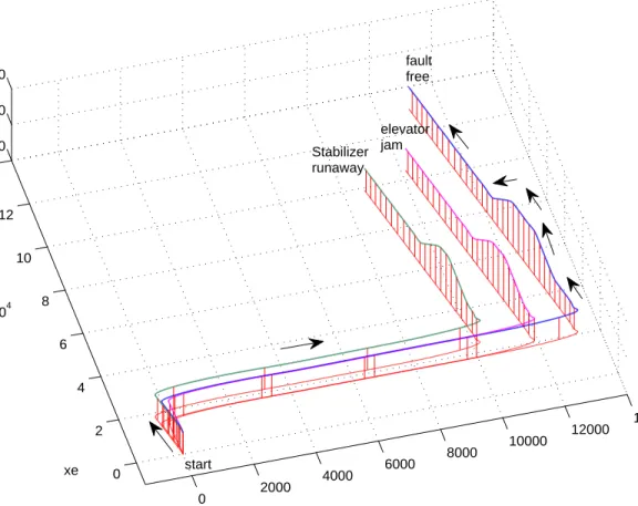
The results in this section represent evaluation tests by an experienced commercial pilot. Figure 3 shows the overall manoeuvres for three different tests: fault-free, elevator jam and stabilizer runaway. The following describes the sequence of manoeuvres conducted during the pilot evaluation:
1) Straight and level flight at 250 kts (128.6m/s), 2000 ft (609.6m) heading North. 2) Insert failure (for failure cases).
3) Right turn 90 deg (East).
4) Left turn back to 0 deg (North). 5) Altitude change to 4000 ft (1219.2m). 6) Altitude change back to 2000 ft (609.6m).
7) Acceleration to 300 kts (154.3m/s) (indicated air speed). 8) Deceleration to 250 kts (128.6m/s) (indicated air speed). 9) Deceleration to 228 kts (117.3m/s) (indicated air speed).
Note that each manoeuvre is allowed to reach steady state before the next sequence is tested.
Remark:Note, although the controller is designed based on the LPV model from [20], the SRS evaluation is based on the high fidelity nonlinear aircraft model [12].
Remark: The controller has been tested at the trim condition
[5.53deg,0.0017deg/s,133.8m/s,5.53deg,600m]
with an input trim [2deg,−1.59deg,45568N] with an initial mass of 317000kg and with the flaps fully retracted. This represents one of the trim conditions used for the GARTEUR FM-AG16 benchmark problem and it is different to the trim conditions of the LPV model in [20]. Using different flight conditions for the evaluation, highlights the capability of the proposed controller to operate in regions away from the design point.
2
If this information is not available, observer based schemes could be employed to estimate the parameters: see for example [22], [23], [24].
0 2 4 6 8 10 12 14 x 104 0 2000 4000 6000 8000 10000 12000 14000 0 1000 2000 ye xe he fault free start elevator jam Stabilizer runaway
Fig. 3. Pilot evaluation: Trajectory
Remark: Note that the aircraft trajectories for the three different tests in Figure 3 are not identical. This is due to the fact that the manoeuvres were ‘manually’ flown by the pilot using the mode control panel. Although the magnitudes of the heading, altitude and speed commands are the same, the times at which each manoeuvre is executed are different.
A. Pilot Evaluation: fault-free
Figure 4 shows longitudinal fault-free performance. The longitudinal states and the tracking performance is shown in Figure 4(a). Figure 4(b) shows the control surface deflections during nominal fault-free conditions. Figure 4(c) shows that no fault/failure is present in the elevator or stabilizer (the actuator effectiveness isW = 1 for both surfaces). Finally Figure 4(d) shows the nominal variation in the switching function and the adaptive gain due to changes in the operating conditions.
B. Pilot Evaluation: elevator jam
Figure 5 shows the pilot evaluation for the case of an elevator jam. Figure 5(c) shows the elevator failure occurred at approximately 63sec when the effectiveness level drops to zero. The effect of the elevator jam can be seen in Figure 5(b). After this point in time, the stabilizer becomes more active in order to compensate for the jammed elevator. Despite the presence of a failure, Figure 5(a) shows similar state tracking performance as the fault-free case. Finally Figure 5(e) shows the switching function is still close to zero indicating sliding is still maintained. Figure 5(d) shows a magnified portion of the estimate
0 200 400 600 800 1000 120 130 140 150 160 Vtas (m/sec) 0 200 400 600 800 1000 500 1000 1500 altitude (m) time (sec) 0 200 400 600 800 1000 −4 −2 0 2 4 Longitudinal states FPA (deg) γ cmd Vtas cmd 0 200 400 600 800 1000 −5 0 5
pitch rate (deg/sec)
0 200 400 600 800 1000
2 4 6 8
angle of attack (deg)
0 200 400 600 800 1000 2 4 6 8 10 pitch (deg) alt cmd
(a) Longitudinal states
0 200 400 600 800 1000 0 2 4 6 elevator (deg) time (sec) 0 200 400 600 800 1000 −3 −2 −1 0
horizontal stabilizer (deg)
time (sec)
ctrl surf defln ctrller u(t)
(b) Longitudinal control surfaces
0 200 400 600 800 1000 0 0.5 1 time (sec) W elevator 0 200 400 600 800 1000 0 0.5 1 time (sec) W horizontal stabilizer
(c) control surface effectiveness estimation
0 200 400 600 800 1000
1 1.5 2
LONG adapt gain
κ (t) time (sec) 0 200 400 600 800 1000 0 0.5 1 Long || σ (t)|| time (sec) (d) switching function and adaptive gain Fig. 4. Pilot evaluation - fault-free longitudinal performance
0 200 400 600 800 120 130 140 150 160 Vtas (m/sec) 0 200 400 600 800 500 1000 1500 altitude (m) time (sec) 0 200 400 600 800 −4 −2 0 2 4 Longitudinal states FPA (deg) states cmd states cmd 0 200 400 600 800 −5 0 5
pitch rate (deg/sec)
0 200 400 600 800
2 4 6 8
angle of attack (deg)
0 200 400 600 800 2 4 6 8 10 pitch (deg) states cmd (a) states 0 200 400 600 800 −2 0 2 4 6 elevator (deg) time (sec) 0 200 400 600 800 −3 −2 −1 0
horizontal stabilizer (deg)
time (sec) ctrl surf defln ctrller u(t) (b) control surfaces 0 200 400 600 800 0 0.5 1 time (sec) W elevator 0 200 400 600 800 0 0.5 1 time (sec) W horizontal stabilizer
(c) control surface effectiveness estimation
50 55 60 65 70 75 80 −0.2 0 0.2 0.4 0.6 0.8 1 1.2 time (sec) W elevator
actual failure time estimated W elevator
(d) zoomed in elevator estimated effectiveness level estimation
0 200 400 600 800 1
1.5 2
LONG adapt gain
κ (t) time (sec) 0 200 400 600 800 0 0.5 1 Long || σ (t)|| time (sec)
(e) switching function and adaptive gain Fig. 5. Pilot evaluation - Elevator jam
0 200 400 600 800 120 130 140 150 160 Vtas (m/sec) 0 200 400 600 800 500 1000 1500 altitude (m) time (sec) 0 200 400 600 800 −4 −2 0 2 4 Longitudinal states FPA (deg) states cmd states cmd 0 200 400 600 800 −5 0 5
pitch rate (deg/sec)
0 200 400 600 800
2 4 6 8
angle of attack (deg)
0 200 400 600 800 2 4 6 8 10 pitch (deg) states cmd (a) states 0 200 400 600 800 −20 −10 0 10 20 elevator (deg) time (sec) 0 200 400 600 800 −10 −5 0 5 10
horizontal stabilizer (deg)
time (sec) ctrl surf defln ctrller u(t) (b) control surfaces 0 200 400 600 800 0 0.5 1 time (sec) W elevator 0 200 400 600 800 0 0.5 1 time (sec) W horizontal stabilizer
(c) control surface effectiveness estimation
0 200 400 600 800
1 1.5 2
LONG adapt gain
κ (t) time (sec) 0 200 400 600 800 0 0.5 1 Long || σ (t)|| time (sec) (d) switching function and adaptive gain Fig. 6. Pilot evaluation: Stabilizer runaway
of the elevator effectiveness levels in the case of the elevator fault in Figure 5(c). Figure 5(d) shows that the estimation provided by the FDI scheme considered in this paper (from page 265 of [7]) is not perfect and includes detection delays (arising from the moving window of information and the filters employed to ensure a usable estimate of the actuator effectiveness levels).
C. Pilot Evaluation: stabilizer runaway
Figure 6 shows the evaluation results for the more challenging case of a stabilizer runaway at approxi-mately 74sec (see Figure 6(c)). The effect of the stabilizer runaway can be seen in Figure 6(b), where the stabilizer runs-away at its maximum rate to the maximum physical limits of 3deg. Figure 6(b) also shows the deflection of the elevator to approximately -10deg immediately after the stabilizer saturates in order to compensate for the stabilizer runaway. Despite the presence of this critical failure, Figure 6(a) shows hardly any noticeable difference in terms of state tracking performance as compared to the fault-free case. Figure 6(d) shows that sliding is still being maintained, and the adaptive gain remains low.
D. Piloted Evaluation: pilot feedback
The following observations and discussions represent feedback from the pilot and the SRS researcher conducting the evaluation for all the three scenarios. Generally, the feedback from the pilot and the SRS researcher indicates that all three tests (nominal, the elevator jam and the stabilizer runaway) showed very similar performance and the pilot was unable to discern a meaningful difference, without looking at the surface deflections. The pilot reported that no transients were observed at the time of the failures. (In fact the SRS researcher had to double check that failures did actually occur).
Some specific comments from the pilot and SRS researcher on the performance of the longitudinal controller are:
• Speed capturing was satisfactory, with some creep towards the set speed at the end (which is acceptable).
• Altitude change capturing resulted in a rather careful 1400 feet per minute rate for a 2000 ft change. A rule of thumb is 2000 ft/min for a 2000 ft change. A small overshoot of 60 ft was observed on both climb and descent, which though not excessive, would not be acceptable in practice. The altitude set point was passed at around 600 ft/min. The subsequent undershoot of 20 ft is also not desirable. A first-order response with no overshoot or undershoot is desirable, rather than the current damped second order response.
• Speed tracking was acceptable during the manoeuvres (1 or 2 kts deviations were observed, which is acceptable).
• Altitude tracking was generally good, apart from the small 40ft (12.2m) drop during heading capture. VII. CONCLUSION
This paper has presented an LPV based FTC scheme using integral sliding modes and control allocation. The scheme proposed in the paper extends the ideas of existing work for LTI systems via an LPV methodology in order to cover a wide range of operating conditions. The integral sliding mode approach was considered to ensure ideal sliding throughout the closed-loop system response, and to maintain nominal performance and robustness in the face of possible actuator faults/failures. Control allocation is used to distribute the ‘virtual’ control signal from the controller to the available redundant actuators especially in the event of faults/failures. The paper also provides a closed-loop stability analysis for a wide range of operating conditions even in the event of certain classes of faults/failures in the actuators. The scheme also takes into account imperfect estimation of the actuator effectiveness levels and considers an adaptive gain for the nonlinear discontinuous part of the control law. The proposed FTC scheme has been implemented and evaluated on the 6-DOF SIMONA research flight simulator in a realistic operational environment to highlight the potential of the scheme for industrial implementation and to highlight the efficacy of the proposed scheme. Evaluation results from the SIMONA research simulator show good tracking performance even in the event of faults/failures.
REFERENCES
[1] S. Yin, H. Luo, and S. X. Ding, “Real-time implementation of fault-tolerant control systems with performance optimization,”IEEE Trans. Ind. Electron., vol. 61, no. 5, pp. 2402–2411, 2014.
[2] H. Yang, B. Jiang, and M. Staroswiecki, “Observer-based fault tolerant control for a class of switched nonlinear systems,”IET Control Theory Appl., vol. 1, no. 5, pp. 1523–1532, 2007.
[3] M. Benosman and K. Lum, “Passive Actuators Fault-Tolerant Control for Affine Nonlinear Systems,” IEEE Trans. Control Syst. Technol., vol. 18, no. 1, pp. 152–163, 2010.
[4] H. Alwi and C. Edwards, “Fault tolerant longitudinal aircraft control using non-linear integral sliding mode,”IET Control Theory Appl., doi: 10.1049/iet-cta.2013.1029, 2014.
[5] M. Rodrigues, D. Theilliol, S. Aberkane, and D. Sauter, “Fault tolerant control design for polytopic LPV systems,”Int. J. Appl. Math. Comput. Sci., vol. 17, no. 1, pp. 27–37, 2007.
[6] I. Szaszi, A. Marcos, G. Balas, and J. Bokor, “Linear Parameter-Varying Detection Filter Design for a Boeing 747-100/200 Aircraft,”
J. Guid. Control Dynam., vol. 28, no. 3, p. 461470, 2005.
[7] H. Alwi, C. Edwards, and C. P. Tan,Fault Detection and Fault–Tolerant Control Using Sliding Modes, ser. AIC. Springer-Verlag, 2011.
[8] H. Alwi and C. Edwards, “Fault tolerant control using sliding modes with on-line control allocation,”Automatica, vol.44, pp.1859-1866, 2008.
[9] M. T. Hamayun, C. Edwards, and H. Alwi, “Design and Analysis of an Integral Sliding Mode Fault Tolerant Control Scheme,”IEEE Trans. Autom. Control, vol. 57, no. 7, pp. 1783–1789, 2012.
[10] S. Sivrioglu and K. Nonami, “Sliding mode control with time-varying hyperplane for amb systems,” IEEE/ASME Trans. Mechatron., vol. 3, no. 1, pp. 51–59, 1998.
[11] H. Alwi, C. Edwards, and A. Marcos, “Fault Reconstruction Using a LPV Sliding Mode Observer for a Class of LPV Systems,” J. Franklin Inst., vol. 349, no. 2, pp. 510–530, 2012.
[12] C. Edwards, T. Lombaerts, H. Smaili, and (Eds.), Fault Tolerant Flight Control: A Benchmark Challenge. Springer-Verlag: LNCIS 339, 2010.
[13] F. Castanos and L. Fridman, “Analysis and design of integral sliding manifolds for systems with unmatched perturbations,”IEEE Trans. Autom. Control, vol. 51, no. 5, pp. 853–858, 2006.
[14] H. Khalil,Nonlinear Systems. Prentice Hall, 1992.
[15] A. Levant and L. Alelishvili, “Integral high-order sliding modes,” IEEE Trans. Autom. Control, vol. 52, no. 7, pp. 1278–1282, 2007. [16] C. Evangelista, P. Puleston, F. Valenciaga, and L. M. Fridman, “Lyapunov-designed super-twisting sliding mode control for wind energy
conversion optimization,”IEEE Trans. Ind. Electron., vol. 60, no. 2, pp. 538–545, 2013.
[17] M. V. Basin and P. C. R. Ram´ırez, “A supertwisting algorithm for systems of dimension more than one,” IEEE Trans. Ind. Electron., vol. 61, no. 11, pp. 6472–6480, 2014.
[18] J. M. A.-D. Silva, C. Edwards, and S. K. Spurgeon, “Sliding-mode output-feedback control based on LMIs for plants with mismatched uncertainties,”IEEE Trans. Ind. Electron., vol. 56, no. 9, pp. 3675–3683, 2009.
[19] P. Apkarian, P. Gahinet, and G. Beck, “Self-scheduledH∞control of linear parameter varying systems: a design example,”Automatica, vol. 31, no. 9, pp. 1251–1261, 1995.
[20] T. H. Khong and J. Shin, “Robustness Analysis of Integrated LPV-FDI Filters and LTI-FTC system for a Transport Aircraft,” inAIAA GNC Conf., AIAA 2007-6771, 2007.
[21] D. Bri`ere and P. Traverse, “Airbus A320/A330/A340 electrical flight controls: A family of fault-tolerant systems.” Digest of Papers FTCS-23 Int. Symposium on Fault-Tolerant Computing, pp. 616–623, 1993.
[22] Q. Ahmed and A. Bhatti, “Estimating SI engine efficiencies and parameters in second-order sliding modes,”IEEE Trans. Ind. Electron., vol. 58, no. 10, pp. 4837–4846, 2011.
[23] F. Caliskan, Y. Zhang, N. E. Wu, and J. Shin, “Actuator fault diagnosis in a Boeing 747 model via adaptive modified two-stage Kalman filter,”J. Aerosp. Eng., vol. 2014, no. ID 472395, 2014.
[24] X. Yan and C. Edwards, “Adaptive sliding mode observer-based fault reconstruction for nonlinear systems with parametric uncertainties,”
IEEE Trans. Ind. Electron., vol. 55, pp. 4029–4036, 2008.
[25] P. Goupil, “Oscillatory failure case detection in the A380 electrical flight control system by analytical redundancy,”Control Eng. Pract., vol. 18, no. 9, pp. 1110–1119, 2010.
[26] —, “AIRBUS state of the art and practices on FDI and FTC in flight control system,”Control Eng. Pract., vol.19, no.6, pp.524-539, 2011.
[27] H. Alwi, C. Edwards, O. Stroosma, and J. A. Mulder, “Evaluation of a sliding mode fault-tolerant controller for the El Al incident,”
H. Alwiwas born in Malaysia. He studied at the University of Leicester and graduated in 2000 with a B.Eng. (Hons) in Mech. Engineering. From 2000-2004 he was an engineer at The NSTP (M) Bhd. In 2004 he moved back to the University of Leicester and was awarded a Ph.D. in 2008 in the area of fault tolerant control applied to aerospace systems. He is the co-author of over 60 refereed papers and a monograph on sliding mode control: Fault Detection and Fault Tolerant Control using Sliding Modes, Springer-Verlag (2011). He is currently a Lecturer at the College of Engineering, Mathematics and Physical Sciences, University of Exeter.
C. Edwards graduated from Warwick University with a B.Sc. (Hons) in Mathematics in 1987 and was awarded a Ph.D. in control from the University of Leicester in 2005. He is a Professor of Control Engineering in the College of Engineering, Mathematics and Physical Sciences at the University of Exeter, UK. His current research interests are in sliding mode control and observation, and their application to fault detection and fault tolerant control problems. He is the co-author of 300 refereed papers in these areas, and three books: Sliding mode control: theory and applications, Taylor & Francis (1998), Fault Detection and Fault Tolerant Control using Sliding Modes, Springer-Verlag (2011) and Sliding Mode Control and Observation, Birkhauser (2013). In addition he recently co-edited the monograph Fault Tolerant Flight Control: a Benchmark Challenge, Springer-Verlag (2010). His is currently vice-chair of the IEEE technical committee on Variable structure systems.
O. Stroosma received the M.Sc. degree in aerospace engineering from Delft University of Technology, Delft, The Netherlands, in 1998. He joined that University’s research lab for Simulation, Motion, and Navigation (SIMONA) and worked on the development of the SIMONA Research Simulator. He is now a researcher at the Control and Simulation group of the Faculty of Aerospace Engineering, Delft University of Technology, as well as technical director of the SIMONA laboratory. His research interests include simulator technology and human-machine interaction in general, and simulator motion cueing and aircraft handling qualities in particular.
J. A. (Bob) Muldergraduated as commercial transport pilot at the RLS civil flight academy in 1967. He received the M.Sc. degree in aerospace engineering (Hons) and the Ph.D. degree in aerodynamic model identification (Hons) from Delft University of Technology, The Netherlands, in 1968 and 1986 respectively, and was appointed Full Professor in 1989. He is (co)author of more than 200 conference and journal papers on subjects ranging from human - machine interface design and cybernetics to identification, estimation, and flight control. He combined his position as chair of the section Control and Simulation and part time captaincies on the Boeing 757-200 and the Boeing 767-300ER, gathering more than 9000 flying hours.
M. T. Hamayun was born in Pakistan. He graduated from Eastern Mediterranean University TRNC Turkey with a B.Sc. and M.Sc (Hons) in Electrical Engineering in 1999 and 2001 respectively, supported by EMU Turkey. In 2001 he joined the Daimler Chrysler AG Research centre Frankfurt Germany. He was awarded a Ph.D from Leicester University in 2013, supported by a CIIT scholarship. He is the co-author of over 20 refereed papers. Currently he is working as Assistant Professor in the Department of Electrical Engineering CIIT Lahore. His research interests include sliding mode control and observation and their applications to fault tolerant control.