Interval-valued analysis for discriminative gene selection and tissue sample
classi
fi
cation using microarray data
Yunsong Qi
⁎
, Xibei Yang
School of Computer Science and Engineering, Jiangsu University of Science and Technology, Zhenjiang, Jiangsu 212003, China
a b s t r a c t
a r t i c l e i n f o
Article history: Received 10 April 2012 Accepted 10 September 2012 Available online 20 September 2012 Keywords:
Microarray Gene selection Classification Rough sets
Interval-valued decision table
An important application of gene expression data is to classify samples in a variety of diagnosticfields. However, high dimensionality and a small number of noisy samples pose significant challenges to existing classification methods. Focused on the problems of overfitting and sensitivity to noise of the dataset in the classification of microarray data, we propose an interval-valued analysis method based on a rough set technique to select discriminative genes and to use these genes to classify tissue samples of microarray data. Wefirst select a small subset of genes based on interval-valued rough set by considering the preference-ordered domains of the gene expression data, and then classify test samples into certain classes with a term of similar degree. Exper-iments show that the proposed method is able to reach high prediction accuracies with a small number of select-ed genes and its performance is robust to noise.
© 2012 Elsevier Inc. All rights reserved.
1. Introduction
Microarray technology allows simultaneous measurement of the expression levels of thousands of genes within a biological tissue sam-ple. An important application of gene expression is to classify samples according to their gene expression profiles, such as the diagnosis or the classification of different types or subtypes of cancer[1,2]. Different classification methods from statistical and machine learning have been applied to the classification of cancer. However, high dimensionality and a small number of noisy samples pose great challenges to the existing methods. The main approach to this problem has been based on using the existing algorithms to analyze gene expression data. For example, support vector machines (SVM)[3], neural networks (NN) [4], logistic regression (LR) [5] and k-nearest neighbor (k-NN) [6] have all been utilized. Most of these classifiers involve complex models containing numerous genes. This has limited the interpretability of the classifiers and this lack of interpretability hampers the acceptance of diagnostic tools. Classification models based on numerous genes can also be more difficult to transfer to other assay platforms, which may be more suitable for clinical application. Several authors have suggested that simple models could perform well in areas such as microarray based cancer prediction [7–9,2]. Investigations have indicated that classifiers could be developed to contain a few genes that provide clas-sification accuracy comparable to that achieved by models that are more complex. Moreover, some more complex algorithms based on numerous genes for classification often overfit the data[10–12].
Prior to classification, a variety of gene selection strategies have been used. The aim of gene selection is to select a small subset of genes from a larger pool. Gene selection methods are classified into three types: (1)filter methods, (2) wrapper methods, and (3) embedded methods. Filter methods evaluate a subset of genes by looking at the intrinsic characteristics of data with respect to class labels, while wrapper methods evaluate the goodness of a gene subset by the accuracy of its learning or classification. Embedded methods are generally referred to as algorithms, where gene selection is embedded in the construction of the classifier. In the gene selection process, an optimal feature subset is always relative to a certain criterion. Every criterion measures the dis-criminating ability of a gene or a subset of genes to distinguish different class labels. To measure the gene–class relevance, different statistical and theoretical measures such as thet-test, entropy and mutual infor-mation are typically used[13–15], and different metrics including the Euclidean distance and correlation coefficient[16,17]are employed to calculate the gene–gene redundancy. However, as thet-test, Euclidean distance, and the correlation coefficient depend on the actual gene expression values of the microarray data, they are very sensitive to noise or outliers within the dataset[18,19].
Rough set theory is a new paradigm to address uncertainty, vague-ness, and incompleteness[20]. It has been applied to a number of methods, including the fuzzy rule extraction, reasoning with uncertain-ty, fuzzy modeling, feature selection and microarray data analysis [21,22,6,23–25,14]. Rough set theory was initially developed for afinite universe of discourse in which the knowledge base is a partition, obtained by any equivalence relationship defined on the universe of discourse. In rough set theory, the data are organized in a table, known as a decision table. Rows of the decision table correspond to objects, and columns correspond to attributes. In the dataset, a class ⁎ Corresponding author. Tel.: +86 511 84409018; fax: +86 511 84404905.
E-mail address:[email protected](Y. Qi).
0888-7543/$–see front matter © 2012 Elsevier Inc. All rights reserved.
http://dx.doi.org/10.1016/j.ygeno.2012.09.004
Contents lists available atSciVerse ScienceDirect
Genomics
label indicates the class to which each row belongs. The class label is termed a decision attribute; the remaining attributes are termed condi-tion attributes. Rough set theory distinguishes itself from other machine learning and pattern recognition methods through three notions of indiscernibility, approximation, and reduction of attributes (introduced inSections 2.2 and 3.4). Thefirst defines a relationship stating that two objects are only equivalent under a selection of attributes. The second gives the ability to define an unknown set of boundaries through the analysis of how that set relates to the objects in the universe. The third allows for the reduction of irrelevant information, thus saving valuable resources. These three important concepts give rough set theory an advantage over other classical methods as it does not need any prelimi-nary or additional information about the data: for example, probability in statistics or grade of membership or the value of possibility in fuzzy set theory, all require further information. The characteristics of the microar-ray data—small sample size and very large dimensionality, create new challenges in obtaining preliminary information.
In practice, discretization is a common preprocess before rough set based mining on gene expression data, which transforms continuous gene expression levels to categorical item sets[26,27]. If a particular gene's expression level is higher than the discretization threshold, the gene is considered as expressed, otherwise it is considered unexpressed. Obviously, a lot of information is lost in the above trans-formation of the dataset with the noise, which is especially inherent in the microarray data[28]. Previous research has shown that handling uncertainty in such applications by the representation as interval data leads to accurate learning algorithms[29,30].
In this study, we propose an interval-valued analysis method to select discriminative genes, and to use these genes to classify tissue samples of microarray data. Wefirst select a small subset of genes based on interval-valued rough set by considering the preference-ordered domains of the gene expression data, and then classifying a test sample into a certain class with a term of similar degree.
To summarize the process:
• The interval-valued decision table of the microarray is generated. In the decision table, each row corresponds to a class of tissue samples, and each column (condition attribute) corresponds to a gene's expression value over all classes of samples. To generate the decision table, the decision attribute is the average gene expression value of a class, and the condition attribute is the value of the 1st quartile and the 3rd quartile of the gene expression value within a class. • In the gene selection step, our objective is to determine the reducts
that discern between objects belonging to different classes. The reduct, from rough set theory, corresponds to a minimal subset of dis-criminative genes. The ordered process of this algorithm is described inSection 4.1.
• The tissue sample classification is based on the selected genes. The proposed interval-valued classification method classifies a sample into a class with the maximum similar degrees.
To facilitate our discussion, wefirst present the basic notions in Section 2.Section 3presents the discernibility approach to compute reducts from the compared dominance relationships. InSection 4, we describe our gene selection and tissue sample classification method. In Section 5, we apply our approach to the analysis of real microarray data. In this section, we also discuss RNA-sequencing data, the data from next-generation sequencing technologies, and analysis using the proposed method. Finally,Section 6, summarizes our approach and pre-sents our conclusions.
2. Preliminaries
2.1. Microarray dataset
A microarray dataset is a gene expression matrix, in which each column represents a gene and each row represents a sample (or
experiment) with a class label. LetG= {g1,⋯,gn} be a set of genes
andU= {s1,⋯,sm} be a set of samples. The corresponding gene
expres-sion matrix can be represented asX¼ xi;j mn, wherexi,jis the
expres-sion level of genegjin samplesi, and usuallyn≫m. Heremis the
number of samples, andnis the number of genes. The matrixXis com-posed ofmrow vectorssi∈Rn,i= 1, 2,⋯,m. Each vectorsiin the gene
expression matrix may be regarded as a point inn-dimensional space, and each of thencolumns consists of anm-element expression vector for a single gene.
A microarray dataset can be regarded as a decision table S¼ bU;AT∪d;V;f >, whereUdenotes the set of samples,ATdenotes the set of the condition attributes (genes),ddenotes the decision attribute (class label),Vis the domain ofAT∪d, andxi,j=f(si,gj).
2.2. Rough set
An information system is a 4-tuple, whereS¼bU;A;V;f >.Uis a non-empty and finite set of objects, called as universe; A is a non-empty andfinite set of attributes, such that∀a∈A:U→Va, where Vais the domain of attributea;Vis regarded as the domain of all
attri-butes such thatV=VA=∪a∈AVa;f(x,a) is the value thatxholds on a(∀x∈U,a∈A).
A decision table is an information system S¼bU;AT∪d;V;f>, whered∉AT.dis a complete attribute called a decision, andATis the condition attribute set.
For an information systemS, it is possible to describe relationships between objects through their attribute values. With respect to a subset of attributes such thatA AT, an indiscernibility relationshipIND(A)[31] may be defined as:
IND Að Þ ¼nðx;yÞ∈U2:∀a∈A;f xð;aÞ ¼f yð;aÞo:
IND(A) is an equivalence relationship because it is reflexive, sym-metrical and transitive. With the relationshipIND(A), two objects are considered to be indiscernible if, and only if, they have the same value on eacha∈A.
Based on the indiscernibility relationshipIND(A), it is possible to derive the lower and upper approximations of an arbitrary subsetX
ofU, which are defined as[31]: A Xð Þ ¼ x∈U:½ xA⊂X
and A Xð Þ ¼x∈U:½ xA∩X≠ϕ
respectively, where [x]A= {y∈U: (x,y)∈IND(A)} is theA-equivalence
class containingx. The pairhA Xð Þ;A Xð Þiis referred to as the Pawlak rough set ofXwith respect to the subset of attributesA.
2.3. Inclusion degree
A partial order on a setXhas a binary relationship⪯with the fol-lowing properties:x⪯x(reflexive),x⪯yandy⪯ximplyx=y (anti-symmetric),x⪯yandy⪯zimplyx⪯z(transitive).
Definition 1. [32,33]Let (X,⪯) be a partially ordered set. If for any
x,y∈X, there is a real numberIðy=xÞwith the following properties: (1) 0≤Iðy=xÞ≤1; (2)x⪯yimplies Iðy=xÞ ¼1; (3)x⪯y⪯zimplies Iðx=zÞ≤Iðx=yÞ; thenI is called an inclusion degree onX.
For an information systemS,Uis the universe, the collection of all normal fuzzy subsets ofUis denoted byF0ð ÞU. LetF1;F2∈F0ð ÞU, if μF1ð Þx≤μF2ð Þx for all x∈U, then F1 F2. It is well known that
F0ð ÞU;p
ð Þis a partially ordered set.
Definition 2. [34]Suppose thatðF0ð ÞU;pÞis a partially ordered set, then I is an inclusion degree on F0ð ÞU , if the following conditions hold: (1) 0≤IðF2=F1Þ≤1; (2) F1pF2⇒IðF2=F1Þ ¼1; (3) F1F2F3⇒ IðF1=F3Þ≤IðF1=F2Þ, whereF1;F2;F3∈F0ð ÞU .
Proposition 1.[34]IfI1;I2are defined as: (1) I1ðF2=F1Þ ¼ min μF1ð Þx∩μF2ð Þx :x∈U;μF1ð Þ ¼x 1 ; (2) I2ðF2=F1Þ ¼ max μF1ð Þx∩μF2ð Þx :x∈U ;
where F1,F2∈F0(U), thenI1;I2are inclusion degrees on(F0(U),p).
2.4. Fuzzy dominance-based rough set
The Dominance-based Rough Set Approach (DRSA) is a new im-provement of Pawlak's rough set model aimed to deal with information systems with preference-ordered domains of the attributes. Greco et al. further generalized DRSA into a fuzzy environment and then proposed the fuzzy dominance-based rough set [35]. In their generalized approach, the target is a fuzzy set instead of the decision tables.
In the decision tableS, ifAT= {a1,⋯,am} is the set of condition
attri-butes, anddis the decision attribute, then we consider a universe of dis-courseUand m+ 1 fuzzy sets [35], denoted byã1,⋯,ãmand d˜, are
defined onUby means of the membership functions μa˜
i:U→½0;1;i∈f1;⋯;mg and μd˜:U→½0;1:
μa˜iandμd˜represent the values of the objectxwith respect to the condition attributeaiand decision attributed, respectively. Suppose
that we want to approximate the knowledge contained in decisiond
using attributes about {ã1,⋯,ãm}. Then, given the information on ã1,⋯,ãm, the lower approximation of the fuzzy set d˜is a fuzzy set
App a˜1;⋯;˜am;d˜
, whose membership function for eachx∈U, denot-ed byμApp a˜1;⋯;a˜m;d˜ ;x h i , is defined as follows[35]: μApp a˜1;⋯;a˜m;d˜ ;x h i ¼ min Z∈D↑ATð Þx μd˜ð Þz ð1Þ for eachx∈U,DAT↑ (x) is a non-empty set defined by
D↑ATð Þ ¼x y∈U:μa˜ ið Þy ≥μa˜ið Þx for eachai∈AT n o : ð2Þ DAT ↑
(x) is the set of objects dominatingxin terms of the set of con-dition attributes.
The lower approximation μ App a˜1;⋯;a˜m;d˜
;x
h i
can be inter-preted as follows: In the universeU, the following implication holds: If μa˜1ð Þy≥μa˜1ð Þx and μa˜2ð Þy≥μa˜2ð Þx and ⋯ and μa˜mð Þy≥μa˜mð Þx, then μd˜ð Þy≥μ App a˜1;⋯;a˜m;d˜
;x
h i
.
Similarly, given the information on {ã1,⋯,ãm}, the upper
approxi-mation ofd˜is a fuzzy setApp a˜1;⋯;a˜m;d˜
, whose membership func-tion for eachx∈Uis defined as follows[35]:
μ App a˜1;⋯;a˜m;d˜ ;x h i ¼ max Z∈D↓ ATð Þx μd˜ð Þz n o ð3Þ for eachx∈U,DAT ↓
(x) is a non-empty set defined by
D↓ATð Þ ¼x y∈U:μa˜
ið Þy ≤μa˜ið Þx for eachai∈AT
n o
: ð4Þ
DAT↓ (x) is the set of objects dominated byxin terms of the set of
condition attributes.
The upper approximation μ App a˜1;⋯;a˜m;d˜
;x
h i
can be inter-preted as follows: In the universe U, the following implication holds: If μa˜1ð Þy ≤μa˜1ð Þx and μa˜2ð Þy ≤μa˜2ð Þx and ⋯ and μa˜mð Þy ≤ μa˜mð Þx, thenμd˜ð Þy ≤μ App a˜1;⋯;a˜m;d˜ ;x h i . App a˜1;⋯;a˜m;d˜ ;App a˜1;⋯;a˜m;d˜ h i
is referred to as a rough set of the fuzzy setd˜by using attributes about the {ã1,⋯,ãm}. More details
about the properties of
App a˜1;⋯;a˜m;d˜ ;App a˜1;⋯;a˜m;d˜ h i , can be found in Ref.[35].
3. Fuzzy rough set in interval-valued decision table
3.1. Pairwise comparison in interval-valued decision table
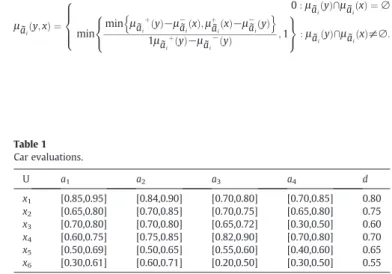
Example 1.To demonstrate the interval-valued decision tables, we considered the data inTable 1, which describes a small training set with interval-valued samples.
Table 1is a summary of the evaluations of cars. This table details six cars, evaluated by means offive attributes:a1: Mileage;a2: Power;a3:
Compression-ratio;a4: Max-speed;d: Global evaluation. The universe
of discourse isU= {x1,⋯,x6},AT= {a1,a2,a3,a4} and is the set of condition
attributes anddis the decision attribute. The global evaluation indicates that the higher the value of a car holds on decisiond, the better the car. Since the similarity measure[36,37]of two interval-valued sets is one of the important topics in valued theory, in the interval-valued decision tableS, let us denote a functionμ:U×U→[0,1] such thatμa˜iðy;xÞ∈½0;1, and it is used to express the degree that an object
yis similar toxon a condition attributeai∈AT. Thus, there are three
possibilities that need to be considered:
• μa˜iðy;xÞ ¼0, i.e.,yis completely not similar toxon attributeai;
•0bμa˜iðy;xÞb1, i.e.,yis partially similar toxwith respect to attribute
aiin degree ofμa˜
iðy;xÞ;
• μa˜iðy;xÞ ¼1, i.e.,yis completely similar toxon attributeai.
The similarity degree discussed here is not necessarily symmetrical, that is,μa˜iðy;xÞ ¼μa˜iðx;yÞdoes not generally hold. It depends on the choice of similarity measurements. By considering the similarity degree of two objects, we consider a universeUandm+ 1 fuzzy set in the interval-valued decision table S, that is,ã1,⋯,ãmand d˜, defined onU
by means of membership functions μa˜i:U→½0;1;i∈f1;⋯;mg and μd˜:U→½0;1.
Example 2.UsingTable 1, we will use the method that was proposed by Leung[38]to compute the similarity degree of two interval-valued values. For eachai∈AT, suppose thatμa˜
ið Þ ¼x μa˜i −ð Þx;μþ ˜ ai x ð Þ h i where μãi −(x) andμ ãi
+(x) represent the lower and upper limitations of the
interval-valued dataμa˜ið Þx respectively, then for∀x,y∈U, the degree thatyis similar toxis defined as:
μa˜iðy;xÞ ¼ 0:μa˜ ið Þy∩μa˜ið Þ ¼x ∅ min min μa˜i þ y ð Þ−μ−a˜ið Þx;μ þ ˜ ai x ð Þ−μ−a˜ið Þy n o 1μa˜iþð Þy−μ ˜ ai −ð Þy ;1 8 < : 9 = ;:μa˜ið Þy∩μa˜ið Þx≠∅: 8 > > < > > : Table 1 Car evaluations. U a1 a2 a3 a4 d x1 [0.85,0.95] [0.84,0.90] [0.70,0.80] [0.70,0.85] 0.80 x2 [0.65,0.80] [0.70,0.85] [0.70,0.75] [0.65,0.80] 0.75 x3 [0.70,0.80] [0.70,0.80] [0.65,0.72] [0.30,0.50] 0.60 x4 [0.60,0.75] [0.75,0.85] [0.82,0.90] [0.70,0.80] 0.70 x5 [0.50,0.69] [0.50,0.65] [0.55,0.60] [0.40,0.60] 0.65 x6 [0.30,0.61] [0.60,0.71] [0.20,0.50] [0.30,0.50] 0.55
The similarity degree for each pair of objects described inTable 1 is displayed in Table 2. For example, μa˜iðx1;x2Þ ¼ a01;
0:17 a2 ; 0:5 a3; 0:67 a4
means thatx1is similar tox2ona1in degree of 0, ona2in degree of
0.17, ona3in degree of 0.5 and ona4in degree of 0.67.
Given that (y,x), (w,z)∈(U×U)2, the pair of objects (y,x) dominate
(w,z) with respect to the set of condition attributesATifyis similar to
x, at least as strong aswis similar tozwith respect to eachai∈AT.
Precisely,“at least as strong as”means the degree ofybeing similar toxis equal to or higher than the degree ofwsimilar toz. Conversely, given (y,x), (w,z)∈U×U, the pair of objects (y,x) is to be dominated by (w,z) with respect to the set of condition attributesATifyis similar toxat most as strong aswis not similar tozwith respect to each
ai∈AT. Similarly,“at most as strong as”means the degree thatyis
similar toxis equal or lower than the degree ofwis similar toz. From the discussion above, by comparing the similarity degrees of different pairs of objects, the dominance relationship can be defined as follows:
Definition 3. Given an interval-valued decision table S, the domi-nance relationship in terms of the set of condition attributesATcan be defined as: RAT¼ ððy;xÞ;ðw;zÞÞ∈ðUUÞ2 :∀ai∈AT;μ˜a iðy;xÞ≥μa˜iðw;zÞ n o :
Unlike the dominance relationship proposed by Greco[39], the dominance relationship presented here is based on the comparison of different pairs of objects. Thus, we call RAT a pairwise compared dominance relationship.
Though the idea of pairwise comparison has been used to form dom-inance relationship by Greco in Ref.[39], our pairwise compared domi-nance relationship is different from Greco's. Greco's domidomi-nance relationship is based on the ordinal properties of preferred degrees of pairs of objects while our approach is based on the ordinal properties of similarity degrees of pairs of objects.
Proposition 2. Given an interval-valued decision tableS, if A AT, then we haveRATpRA.
Proposition2is consistent to the property in the traditional rough set, that is to say, the more attributes we have, thefiner binary rela-tionship we obtained.
3.2. Fuzzy rough approximations
Suppose that we want to approximate the knowledge contained indby using the comparison of pairs of objects, given the infor-mation on {ã1,⋯,ãm}, the lower approximation of d˜ is a fuzzy set
Appσ a˜1;⋯;a˜m;d˜
, whose membership function for each (y,x) ∈U×U, denoted by μAppσ a˜1;⋯;a˜m;d˜ ;ðy;xÞ h i , is defined as fol-lows: μAppσ a˜1;⋯;a˜m;d˜ ;ðy;xÞ h i ¼ min Z∈D↑ ATðy;xÞ μd˜ð Þz n o ð5Þ whereDAT ↑
(y,x) is a non-empty set defined by:
D↑ATðy;xÞ ¼fw∈U:ððw;xÞ;ðy;xÞÞ∈RATg: ð6Þ
DAT↑ (y,x) is set of objects dominatingyin terms of the similarity
degrees ofx. The formulation of Appσ a˜1;⋯;a˜m;d˜
is concordant with the syntax of the decision rules induced by means of DRSA in a pairwise comparison of objects. Thus, the lower approximation mem-bershipμ Appσ a˜1;⋯;a˜m;d˜
;ðy;xÞ
h i
is concordant with the decision rules of the type:If w is similar to x in degree at leastμa˜1ðy;xÞon
attri-bute a1and⋯and w is similar to x in degree at leastμa˜mðy;xÞon
attri-bute am, thenμd˜ð Þw≥μ Appσ a˜1;⋯;a˜m;d˜
;ðy;xÞ
h i
.
Given the information on {ã1,⋯,ãm}, the upper approximation ofd˜
is a fuzzy set Appσ a˜1;⋯;a˜m;d˜
, whose membership function for each (y,x)∈U×U, denoted byμ Appσ a˜1;⋯;a˜m;d˜
;ðy;xÞ h i , is defined as follows: μ Appσ a˜1;⋯;a˜m;d˜ ;ðy;xÞ h i ¼ min Z∈D↓ATðy;xÞ μd˜ð Þz n o ð7Þ whereDAT ↓
(y,x) is a non-empty set defined by:
D↓ATðy;xÞ ¼fw∈U:ððy;xÞ;ðw;xÞÞ∈RATg: ð8Þ
DAT↓(y,x) is a set of objects dominatingyin terms of the similarity
de-grees ofx. The upper approximationμ Appσ a˜1;⋯;a˜m;d˜
;ðy;xÞ
h i
is con-cordant with decision rules of the type:If w is similar to x in degree at most
μa˜1ðy;xÞon attribute a1and⋯and w is similar to x in degree at most μa˜mðy;xÞon attribute am, thenμd˜ð Þw≤μ Appσ a˜1;⋯;a˜m;d˜
;ðy;xÞ h i . Appσ a˜1;⋯;a˜m;d˜ ;Appσ a˜1;⋯;a˜m;d˜ h i is referred to as a pair of rough set of fuzzy knowledge contained in decisiondin terms of the similarity degrees comparison of pairs of objects.
Table 2
Similarity degrees of different cars inTable 1.
μa˜iðy;xÞ a1 a2 a3 a4 a5 a6 x1 1 a1; 1 a2; 1 a3; 1 a4 0 a1; 0:17 a2 ; 0:5 a3; 0:67 a4 0 a1; 0 a2; 0 a3; 0 a4 0 a1; 0:17 a2 ; 0 a3; 0:67 a4 0 a1; 0 a2; 0 a3; 0 a4 0 a1; 0 a2; 0 a3; 0 a4 x2 0 a1; 0:07 a2 ; 1 a3; 0:67 a4 1 a1; 1 a2; 1 a3; 1 a4 0:67 a1 ; 0:67 a2 ; 0:4 a3; 0 a4 0:67 a1 ; 0:67 a2 ; 0 a3; 0:67 a4 0:27 a1 ; 0 a2; 0 a3; 0 a4 0 a1; 0:07 a2 ; 0 a3; 0 a4 x3 0 a1; 0 a2; 0:29 a3 ; 0 a4 1 a1; 1 a2; 0:29 a3 ; 0 a4 1 a1; 1 a2; 1 a3; 1 a4 0:5 a1; 0:5 a2; 0 a3; 0 a4 0 a1; 0 a2; 0 a3; 0:5 a4 0 a1; 0:1 a2; 0 a3; 1 a4 x4 0 a1; 0:1 a2; 0 a3; 1 a4 0:67 a1 ; 1 a2; 0 a3; 1 a4 0:33 a1 ; 0:5 a2; 0 a3; 0 a4 1 a1; 1 a2; 1 a3; 1 a4 0:6 a1; 0 a2; 0 a3; 0 a4 0:07 a1 ; 0 a2; 0 a3; 0 a4 x5 0 a1; 0 a2; 0 a3; 0 a4 0:21 a1 ; 0 a2; 0 a3; 0 a4 0 a1; 0 a2; 0 a3; 0:5 a4 0:47 a1 ; 0 a2; 0 a3; 0 a4 1 a1; 1 a2; 1 a3; 1 a4 0:58 a1 ; 0:34 a2 ; 0 a3; 0:5 a4 x6 0 a1; 0 a2; 0 a3; 0 a4 0 a1; 0:09 a2 ; 0 a3; 0 a4 0 a1; 0:09 a2 ; 0 a3; 1 a4 0:03 a1 ; 0 a2; 0 a3; 0 a4 0:35 a1 ; 0:45 a2 ; 0 a3; 0:5 a4 1 a1; 1 a2; 1 a3; 1 a4
3.3. Some properties
Proposition 3.Given an interval-valued decision tableS, if ApAT, for each(y,x)∈U×U, we have:
DA↑ðy;xÞ ¼∪ D↑ATðw;xÞ:w∈D↑Aðy;xÞ
n o
ð9Þ
D↓Aðy;xÞ ¼∪nD↓ATðw;xÞ:w∈D↓Aðy;xÞo: ð10Þ Proposition3holds due to the transitive of the used pairwise com-parison dominance relationship. Generally, if the used binary relation is reflexive and transitive, then such properties hold no matter what kind of rough approximation is selected.
Proposition 4. Given an interval-valued decision table S, for each
(y,x)∈U×U, we have: μAppσ a˜1;⋯;a˜m;d˜ ;ðy;xÞ h i ¼ I1 D↑ATðy;xÞ ð11Þ μ Appσ a˜1;⋯;a˜m;d˜ ;ðy;xÞ h i ¼ I2 D↓ATðy;xÞ : ð12Þ
Proposition4shows that the proposed rough approximations are equivalent to the inclusion degree presented in Ref.[34]. It presents a relationship between the rough set and included degree.
Proposition 5.Given an interval-valued decision tableS, the following properties are satisfied:
(1) Let us denote by d˜d the Cartesian product on fuzzy set˜ d, that˜ is, for each(y,x)∈U×U, Ud˜ d y˜ð ;xÞ ¼min μd˜ð Þy;μd˜ð Þx
, then Appσ a˜1;⋯;a˜m;d˜ ˜ dd App˜ σ a˜1;⋯;a˜m;d˜ : ð13Þ
(2) For any negation N(⋅), being a strictly decreasing function N: [0,1]→[0,1]such that N(1) = 0and N(0) = 1,
Appσ a˜1;⋯;a˜m;d˜ C ¼ Appσ a˜C1;⋯;a˜ C m;d˜ C ð14Þ Appσ a˜1;⋯;a˜m;d˜ C ¼ Appσ a˜C1;⋯;a˜ C m;d˜ C ð15Þ Appσ a˜1;⋯;a˜m;d˜ C ¼Appσ a˜C1;⋯;a˜ C m; d˜ C ð16Þ Appσ a˜1;⋯;a˜m;d˜ C ¼Appσ a˜C1;⋯;a˜ C m;d˜ C ð17Þ
where for a given fuzzy set W, the fuzzy set WCis the complement of W, defined byμWCð Þ ¼x NðμWð ÞxÞ.
(3) For each set of condition attributes such that a˜1;⋯;a˜l;d˜
n o p a˜1;⋯;a˜m;d˜ n o , Appσ a˜1;⋯;a˜l;d˜ pAppσ a˜1;⋯;a˜m;d˜ ð18Þ Appσ a˜1;⋯;a˜l;d˜ tAppσ a˜1;⋯;a˜m;d˜ ð19Þ (4) If μa˜
iðy;xÞ≥μa˜iðw;xÞfor each ai∈AT, where(y,x), (w,x)∈U×U,
then μhAppσa˜1;⋯;a˜m;d˜;ðy;xÞi≥μhAppσa˜1;⋯;a˜m;d˜;ðw;xÞi ð20Þ μ Appσ a˜1;⋯;a˜m;d˜ ;ðy;xÞ h i ≥μ Appσ a˜1;⋯;a˜m;d˜ ;ðw;xÞ h i : ð21Þ
Results (1), (2), (3) and (4) of Proposition5can be regarded as fuzzy counterparts of results, which is well known in the classical rough set theory. More precisely, (1) shows that the fuzzy setd˜d˜includes its lower approximation and is included in its upper approximation; (2) represents complementarily properties of the proposed fuzzy rough approximations; (3) expresses monotonicity of the proposed fuzzy rough set in terms of the monotonous varieties of condition attri-butes; and (4) says that the lower and upper approximations are mono-tonic with respect to the monomono-tonicity of similarity degree of pairs of objects.
3.4. Attribute reduction
3.4.1. Attribute reduction of pairwise compared dominance relationship
Definition 4. Given an interval-valued decision tableS,ApAT, thenA
is referred to as a reduct ofATin terms of a pairwise compared dom-inance relationship if the following two conditions hold:
(1) RAT¼RA;
(2) RAT≠RBfor eachB⊂A.
A reduct ofATis actually a minimal subset of condition attributes which preserves the pairwise compared dominance relationRAT.
∀(y,x),(w,z)∈(U×U)2, let us denote byRATððy;xÞ;ðw;zÞÞ ¼ a
i∈AT: f y;x ð Þ;ðw;zÞ ð Þ∉Raig ¼ ai∈AT:μaiðy;xÞbμaiðw;zÞ n o , DATððy;xÞ;ðw;zÞÞis referred to as the discernibility attribute sets of pairs (y,x) and (w,z), DAT¼nDATððy;xÞ;ðw;zÞÞ:ðy;xÞ;ðw;zÞ∈ðUUÞ2o
is referred to as the discernibility matrix ofS.
Theorem 1.Given an interval-valued decision tableS, ApAT, for each
DATððy;xÞ;ðw;zÞÞ≠∅, we haveRAT¼RA⇔A∩DATððy;xÞ;ðw;zÞÞ≠∅. 3.4.2. Attribute reduction of fuzzy rough set
The approach of attribute reduction discussed above is with respect to the pairwise compared dominance relationship. In other words, no decision attribute is considered. In the following steps, we will present the practical approach to attribute reductions about fuzzy rough sets. Definition 5. Given an interval-valued decision table S, ApAT= {a1,⋯,am},
(1) A is referred to as a reduct of lower approximation Appσ ˜
a1;⋯;a˜m;d˜
if and only if for each (y,x)∈U×U, (a)I1 d=D↑ATðy;xÞ ¼ I1 d=D↑Aðy;xÞ , (b) I1 d=D↑Bðy;xÞ ≠I1 d=D↑ATðy;xÞ for∀B⊂A;
(2) A is referred to as a reduct of upper approximation Appσ
˜
a1;⋯;a˜m;d˜
if and only if for each (y,x)∈U×U, (a)I2 d=D↓ATðy;xÞ ¼ I2d=D↓Aðy;xÞ, (b) I2 d=D↓Bðy;xÞ ≠I2 d=D↓ATðy;xÞ for∀B⊂A;
Since Proposition4shows that the lower and upper approxima-tions are equal to two different inclusion degrees, we define the reducts of lower and upper approximations based on the inclusion degrees. Obviously, the reducts of lower and upper approximations are minimal subsets of attributes, which preserve the lower and upper approximation memberships for each pair (y,x)∈U×U. Theorem 2.(Judgment Theorem.)Given an interval-valued decision tableS, ApAT, then for each(y,x)∈U×U,
(1) I1 d=D↑ATðy;xÞ
¼ I1d=D↑Aðy;xÞ⇔ifI1d=D↑ATðy;xÞ>I1ðd= DAT↑ ðw;xÞÞthen D↑Aðw;xÞD↑Aðy;xÞ;
(2) I2 d=D↓ATðy;xÞ
¼ I2d=D↓Aðy;xÞ⇔ifI2ðd=D↓ATðw;xÞÞ>I2ðd=
DAT↓ ðy;xÞÞthen D↓Aðw;xÞD↓Aðy;xÞ;
The above theorem provides approaches to judge whether a subset of condition attributes is persevering the lower (upper) approximate membership value for each (y,x)∈U×U. We can further obtain practical approaches to compute lower and upper approximate reducts in the decision table. Wefirst give the following notions.
Definition 6. Given an interval-valued decision tableS, denoted by
DL AT¼ fðw;xÞ;ðy;xÞg:I1 d=D↑ATðy;xÞ >I1 d=D↑ATðw;xÞ n o ; DU AT¼ fðw;xÞ;ðy;xÞg:I2 d=D↓ATðw;xÞ >I2 d=D↓ATðy;xÞ n o ; where, DL ATfðw;xÞ;ðy;xÞg ¼ ai∈AT: w;x ð Þ;ðy;xÞ ð Þ∉Rai : fðw;xÞ;ðy;xÞg∈DL AT AT : fðw;xÞ;ðy;xÞg∉DL AT 8 < : DU ATfðw;xÞ;ðy;xÞg ¼ ai∈AT: y;x ð Þ;ðw;xÞ ð Þ∉Rai : fðw;xÞ;ðy;xÞg∈DU AT AT : fðw;xÞ;ðy;xÞg∉DU AT : 8 < : DL
ATfðw;xÞ;ðy;xÞgandDUATfðw;xÞ;ðy;xÞgare referred to as lower and upper approximate discernibility attribute sets, respectively,DL
AT and DU
AT are referred to as lower and upper approximate discernibility matrices, respectively.
Standard approaches to finding reducts are based on the
discernibility matrix. Usually there are many reducts in an informa-tion system. The intersecinforma-tion of all reducts is called the CORE. In a discernibility matrix, every entry represents a set of attributes dis-cerning two objects. If an entry consists of only one attribute, then it has a higher significance and the unique attribute must be a mem-ber of the CORE. Also, shorter entry is more significant than the longer one. If the times of appearance of an attribute are more than that of the others in the same entry, then this attribute may contribute more classification power to the reduct.
According to the above declaration, we assigned a weightW(ai) to
each attributeai. The value of weightW(ai) for eachai, which is set to
zero initially, is calculated sequentially throughout the whole matrix using the following formula when a new entry Ct is met in the
discernibility matrix:
W að Þ ¼i W að Þ þi kCtj jA=jCtj;ai∈Ct ð22Þ where |A| is the cardinality of attribute setAof the information system, |Ct| is the cardinality of the new entryCt, kCt is the number of the same entryCtin the merged matrix.
The heuristic method is based on the fact that if the dataset is consistent, then the intersection of a reduct and an entry in the discernibility matrix cannot be empty; otherwise, the involved two objects would be indiscernible with respect to the reduct according to the definition of the reduct in which the reduct possesses discern-ible capability for all objects.
Based on the above, we can search reducts with a discernibility matrix.
4. Gene selection and tissue sample classification
As mentioned inSection 2.1, a microarray dataset can be regarded as a decision table. Reducts, from the rough set theory, correspond to a minimal subset of discriminative genes. Our objective is to determine the reducts that can discern between objects belonging to different classes. Tissue sample classification is based on the decision table from the microarray dataset. To generate the decision table, the decision attributedtakes its value from the average of the corresponding condi-tion attribute (gene expression value) of a class, and the condicondi-tion attri-bute takes its value from the 1st quartile and the 3rd quartile of the gene expression value within a class.
4.1. Gene selection
Based on the introduced concept, we present an interval-valued reduct (IVR) method to select the genes. The ordered process of this algorithm is:
Algorithm IVR.
1. Initialize the parameters of the algorithm: the designated output reductRed=∅, weight valuesW(ai) = 0,i= 1,⋯,n.
2. Compute the lower and upper approximate discernibility matrices
DATL orDATU;
3. Form a new discernibility matrix (DATL orDATU), merge all the same
en-tries in the discernibility matrix, record their frequencies and sort all entries in the matrix according to their length (the number of attri-butes involved in each entry) in descending order; if two entries have the same length, the entry with more frequency is preferred. 4. Use formula(22)to compute the weight value of each attribute in
the entry.
5. Calculate the intersectionInSet between the reductRed and an entryCt:InSet=Red∩Ct,t= 1, 2,⋯, whenInSet=∅is obtained go
to the next step.
6. An attributeaiwith the maximal weight value is chosen and added
toRed.
7. It will go back to the intersection calculation and repeat the pro-cess if there is an entry left in the discernibility matrix, otherwise the resulting outputRedis the optimal reduct.
In this paper, if a reduct is calculated fromDL AT DUAT
, it is referred to as the lower(upper) approximate reductRedL(RedU).
4.2. Tissue sample classification
Our interval-valued classification (IVC) method for the microarray is based on the union ofRedLandRedUfrom IVR. Suppose thatμd−(xi,cj)
andμd+(xi,cj) represent the lower and upper approximation similar
degree between samplexiand classcj, [dcj −,d
cj
+] represents the interval
of decision attribute value, let μd(xi,cj) = [μd−(xi,cj),μd+(xi,cj)], dcj¼
d−cj;d þ
cj
h i
, then classify samplexito classck:
k¼ arg max j¼1;2;⋯;5 μ μd xi;cj ;dcj n o ; where, μ μd xi;cj ;dcj ¼min 0 : μd xi;cj ∩dcj¼∅ min μþ d xi;cj −d−cj;d þ cj−μ − d xi;cj n o μþ d xi;cj −μ− d xi;cj ;1 8 < : 9 = ; : μd xi;cj ∩dcj≠∅ 8 > > > < > > > :
5. Experiments
In this section, we present experimental results provided by the IVR and the IVC methods. We evaluate the discriminative performance of our selected gene set on different classifiers. We also compare the per-formance of our classifying method to a wide range of standard
classi-fiers: Naive Bayes (NB),k-NN, Decision Tree (DT) and SVM. We have performed only a limited parameter optimization. For thek-NN classifi -er, three types ofk-NN classifiers (k= 1, 3, 5) were compared to assess the significant performance and we set the parameterkas 3. For the SVM classifier, the linear SVM shows the best performance among the linear, polynomial kernel with exponent 2 and RBF kernel. Since most microarray datasets only have relatively few samples, we chose the leave-one-out cross-validation method for evaluation.
To evaluate our gene selection method IVR, the compared gene sets are selected by the program of Significance Analysis of Microarrays (SAM)[40], a statistical technique forfinding significant genes. For the standard classifiers, deciding the number of discriminative genes to select is thefirst question. A set of experiments are conducted on the dataset by varying the number of genes selected to receive the highest classification accuracy.
Our implementation of the various compared classifiers is based on the Weka environment (http://www.cs.waikato.ac.nz/ml/weka/). The classification accuracy is used as the performance measure. For all the dataset, normalizations are performed so that every observed gene expression has a mean equal to 0 and a variance equal to 1.
5.1. Results on ALL/AML leukemia dataset
To evaluate the performance of our proposed method in practice, we have used a dataset containing gene expression profiles from patients with acute lymphoblastic leukemia (ALL) and acute myelo-blastic leukemia (AML) and compared the ALL/AML dataset with the IVR and the IVC methods.
The ALL portion of the dataset is derived from two cell types, B-cells and T-cells, while the AML part is split into two types, bone marrow (BM) samples and peripheral blood (PB). The dataset was studied in [1]. However, due to the bipartition of each component, it can be treated both as a three-class dataset (B-cell, T-cell, and AML) and as a four-class dataset (B-cell, T-cell, AML-BM, and AML-PB). Here the three-class version is referred to as ALL–AML-3 and the four-class version as ALL– AML-4.Table 3provides a summary of the ALL/AML dataset.
The decision table for ALL–AML-4 dataset is shown inTable 4. The lower and upper approximation reducts are shown inTable 5. Based on these reducts, we can classify a test sample into a certain class. Classification accuracy on ALL–AML datasets are shown inTables 6 and 7. The experimental results show that our proposed methods have a dominating performance. The reason may be that microarrays contain various technical noises. In Subsection 5.3, we design a set of simulations to examine the robustness of our approach to noise.
5.2. Results on NCI-60 dataset
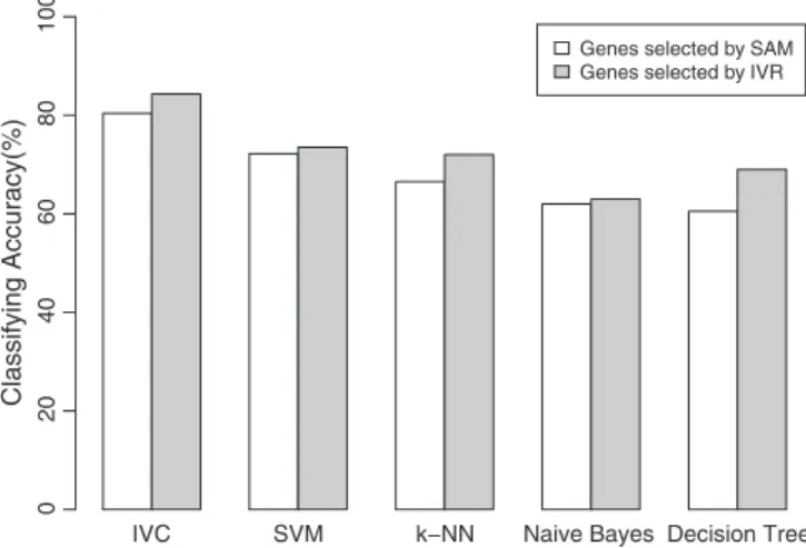
To further test the performance of the proposed method, we applied our algorithm to the National Cancer Institute's anti-cancer drug-screen data (NCI-60) of Ross et al.[41]consisting of 61 samples from human cancer cell lines. The NCI-60 dataset spans nine classes and gene expres-sion levels were measured for 10,000 genes. The prediction accuracy of 66.66% is reported in reference[41]using one-versus-the rest SVM with 150 selected genes. To test our algorithm on an external dataset (independent set), 43 samples are used for the training dataset while 18 samples as testing dataset. Based on 150 genes selected by SAM and 12 genes selected by IVR, we report the classification accuracy of all the compared algorithms withFig. 1. Consistent with the results on leukemia dataset, in this experiment, our proposed method also achieved the highest classification accuracy.
5.3. Simulations for noise sensitivity analysis
High noise is always a challenge in existing gene expression data analysis algorithms. We studied the noise sensitivity property of our method and the standard classifiers on simulated datasets generated by adding artificial noise to real gene expression datasets.
In the experiments, the simulated noise has Gaussian distribution,
N(0,wδj2), whereδj2is thejth gene expression level's variance, and wis the weight of the simulated noise. After adding the generated Gaussian noise, expression levelxjis shifted toxj+N(0,wδj2).
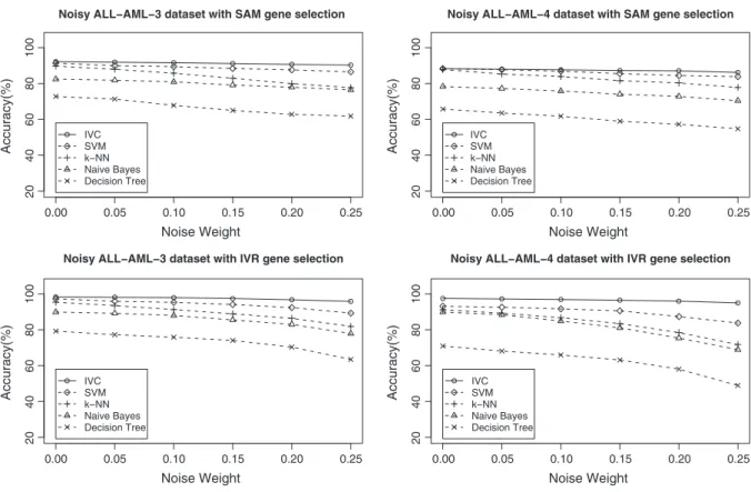
Fig. 2shows the comparison of IVC classifier and standard
classi-fiers against synthetic noise on the ALL–AML datasets. These results show that our IVC method is the most robust method. The IVC meth-od achieves reasonable classification accuracy, even when the data contain a lot of noise. This is because, in our rough set based method, gene expression data are treated as interval-valued data by consider-ing the preference-ordered domains and compared with a term of similar degree, which already takes the noise into consideration. The accuracy of Naive Bayes,k-NN, Decision Tree and SVM decreases dramatically with the increase in noise, meaning that all of the methods are sensitive to noise.
5.4. Discussion
From the results shown inTables 6 and 7, we observe the following: (1) The accuracy of the classification is highly dependent on the choice of the classification method. For instance, with the gene set selected by the IVR method, the IVC classifier has an Table 3
Summary of the ALL/AML dataset.
Dataset Samples Genes Classes
ALL–AML-3 72 7129 3
ALL–AML-4 72 7129 4
Table 4
Decision table of ALL–AML-4 dataset.
U G1 G2 ⋯ G7129 d dinterval c1 [0.0332, 0.1220] [0.0622, 0.1998] ⋯ [0.0314, 0.1183] 0.7223 [0.0655, 1.0000] c2 [0.3246, 0.6484] [0.0464, 0.1436] ⋯ [0.0671, 0.1227] 0.6302 [0.0512, 0.9165] c3 [0.0783, 0.1712] [0.0715, 0.1524] ⋯ [0.0908, 0.1789] 0.5278 [0.0301, 0.7533] c4 [0.0734, 0.1548] [0.0524, 0.1243] ⋯ [0.1050, 0.1733] 0.4309 [0.0186, 0.5296] Table 5
Genes selected in a reduct set of ALL–AML datasets.
Lower approximation reduct Upper approximation reduct
ALL–AML-3 ALL–AML-4 ALL–AML-3 ALL–AML-4
CD33 CD33 CD33 CD33
IL8 IL8 IL8 IL8
ZYX ZYX ZYX ZYX
ASAH1 ASAH1 PSME1 PRSS3
PRSS3 PSME1 PRAME PRAME
accuracy of 97.47% on the ALL–AML-4 dataset, while the accu-racy by Decision Tree is 70.92%. To better understand IVC's performance, we rank the average classification accuracy of all the algorithms throughoutTables 6 and 7as follows: IVC 94ð :05%Þ>SVM 92ð :72%Þ>kNN 91ð :03%Þ>NB 86ð :14%Þ
>DT 72ð :09%Þ:
It is observed that our IVC method gets the best performance. The experimental results on NCI-60 dataset (Fig. 1) are also consis-tent with this.
(2) The accuracy of the classification is also highly dependent on the selected gene set. When the genes are selected by the SAM method, the SVM classifier has an accuracy of 91.41% on the ALL–AML-3 dataset. On the same dataset with the gene set selected by IVR method, the accuracy of SVM is 97.27%. This sig-nificant differential accuracy between the gene selection method of SAM and IVR also occurs with the other classifiers.
(3) Although the number of selected genes with the IVR method is much less than by SAM, the accuracies of all the methods are im-proved on the two ALL/AML datasets. The classification accuracy inTable 6is generally smaller for all algorithms compared to the results inTable 7. Yet the algorithms inTable 7use much less genes for the classification than inTable 6. The main idea of rough set theory is to reduce the redundancy of data by attribute reduction, while preserving the ability of classification. Com-pared with other approaches to attribute reduction, rough set theory can be used to discover data dependencies and reduce the number of attributes contained in a data set by purely struc-tural methods. The reduced set of attribute preserves the under-lying semantics of the features. In theory, a reduct can represent all the discriminative attributes contained in a data. In practice, it is observed that, when the number of selected attributes with purely structural methods is greater than a certain degree, the variation of the classifying accuracy is small[42]. The higher the degree of overlap between the reduct and the selected attri-butes indicates that the higher the percentage of the selected attributes contained the discriminative attributes in a data. (4) When the sample sizes decrease (ALL–AML-3 dataset vs. ALL–
AML-4 dataset), the performance of the IVC classifier is even more outstanding. For example, compared to the SVM classifier,
with the gene set selected by the IVR method, the accuracy of IVC classifier is improved by 4.32% on the ALL–AML-4 dataset, while it is only improved by 1.05% on the ALL–AML-3 dataset. Note that, the number of samples in each class of the ALL– AML-4 dataset is lower than those in the ALL–AML-3 dataset. From the results shown inTables 6 and 7, we can see that the IVC is shown to be the best method for tissue classification based on gene expression. It achieves better performance than any of the other clas-sifiers. It is conceivable that feature selection raises the accuracy since it can reduce the number of insignificant dimensions, thereby over-coming the curse of dimensionality. This appears to be the case for
k-NN, Decision Tree and SVM classifier methods. The accuracy of
k-NN, Decision Tree and SVM is improved on the two datasets with genes selected by the IVR method. The accuracy of the Naive Bayes is also dramatically improved on the experimental datasets. Also, re-markably, with the aid of feature selection, IVC achieves the 98.32% accuracy on the ALL–AML-3 dataset and 97.47% accuracy on the ALL–AML-4 dataset. For the SVM method, it is possible to achieve very high accuracy on most of the microarray datasets[42]. However, the best performance on the experimental datasets does not outperform the IVC method. These two datasets have smaller sample sizes than the other datasets, so one may conclude that multiclass classification based on gene expression can be effectively solved when the sample size is large. Although it has been widely used in text categorization, Naive Bayes reported that it did not appear to perform very well for tissue classification based on gene expression using the standard feature selection method[42]. This is not very surprising, since Naive Bayes is based on the assumption that the fea-tures are conditionally independent given the class label, which may not be the case for gene expression data because of co-regulation. For the IVR method, genes were selected as a reduct without redundancy and results in independence between selected feature genes.
The selected gene set for leukemia classification, including PSME1, CD33, IL8, PRAME, ASAH1, PRSS3, MAL and ZYX, that achieve 97.47% and 98.32% classifying accuracy is experimentally proved to be corre-lated to leukemia of ALL or AML. Specifically, Gene PSME1 inhibits programmed cell death and promotes survival of C-cell chronic lym-phocytic leukemia (B-CLL) cells in culture[43]. By delaying apoptosis, PSME1 may extend the life span of the malignant cells. The human differentiation antigen CD33 is a marker of leukemia (ALL) and also a member of the sialic acid-binding immunoglobulin-like lectin (Siglec) family of inhibitory receptors. It is also a therapeutic target
for AML [44]. Gene IL8 was found to be up regulated in human
Table 6
The classification accuracy with gene set selected by SAM method.
Classifier Number of selected genes Classification accuracy
ALL–AML-4 ALL–AML-3 ALL–AML-4 ALL–AML-3
Naive Bayes 80 85 78.33% 82.44% k-NN 40 50 87.81% 89.73% Decision Tree 60 55 65.35% 72.78% SVM 85 100 89.04% 91.41% IVC 30 30 88.25% 92.17% Table 7
The classification accuracy with gene set selected by IVR method.
Classifier Number of selected genes Classification accuracy
ALL–AML-4 ALL–AML-3 ALL–AML-4 ALL–AML-3
Naive Bayes 8 7 89.87% 93.93%
k-NN 8 7 91.22% 95.36%
Decision Tree 8 7 70.92% 79.29%
SVM 8 7 93.15% 97.27%
IVC 8 7 97.47% 98.32%
1. The selected gene set is the union of lower and upper approximation reduct. 2. Note that some genes appear in both lower and upper approximation reduct.
IVC SVM k−NN Naive Bayes Decision Tree
Genes selected by SAM Genes selected by IVR
Classifying Accuracy(%) 0 2 0 4 0 6 0 8 0 100
Fig. 1.The comparison of classifying accuracy on NCI-60 dataset with 150 genes select-ed by SAM and 12 genes selectselect-ed by IVR.
T-cell acute lymphoblastic leukemia[45]. Overexpression of the pref-erentially expressed antigen PRAME of melanoma was found in 62% (n= 31) of 50 patients with higher rates of overall and disease-free survival from AML. PRAME expression at diagnosis was negatively correlated to the white blood cell count (Pb0.05), which was signifi -cantly higher in patients with t(8;21) and corresponded with those at relapse (Pb0.001), suggesting that its expression is an indicator of fa-vorable prognosis, and could be a useful tool for monitoring minimal residual disease in childhood AML[46]. The gene ASAH1 is correlated to the survival of cytotoxic lymphocytes[47]. The serine protease family member PRSS3 is a putative tumor suppressor gene due to its loss of expression in acute lymphoblastic leukemia [48] and other tumors. It may be functionally important as a serine protease in tumor development. The MAL gene is related to T-cell ALLs[49]. ZYX is a gene correlated to leukemia of ALL[50]. It is also localized at focal contacts in adherent erythroleukemia cells[51].
From the experimental results above, we conclude that our pro-posed approach is superior to other methods. This may be due to the following advantages: interval-valued analysis, minimum redundancy of the selected gene subset, and simple classifiers. First, we used interval-valued gene expressions instead of point-valued gene expres-sions. A major challenge in DNA microarray analysis is to eliminate the effects of noise. Our method is non-parametric and has an advan-tage over other methods since no assumption about the nature of the noise is required. Second, the selected gene subset is the union of lower and upper approximation reducts which is actually a minimum redundancy–maximum relevance condition attribute subset. Such a feature set covers the data domain better and improves the perfor-mance of various classifiers [52]. Third, the proposed IVC method classifies a sample to a class with the maximum similar degrees. The IVC method does not need parameter tuning. The small sample size and high dimensionality of the microarray data constrain the possibility of properly validating the chosen classification model. If a complex model was required to tune many parameters, a large computational effort would be required, compounded with a high risk of overfitting.
Although the proposed method was originally designed for mi-croarray data analysis, it can be applied to the data from the next-generation sequencing technologies. Recently, high-throughput RNA sequencing (RNA-seq) has emerged as a powerful new technology for transcriptome analysis [53]. By mapping millions of RNA-seq reads to individual gene transcripts, it is possible to estimate the overall mRNA abundance and detect DEGs[54]. Currently, most of the methodologies proposed so far rely on parametric assumptions and use Poisson or negative binomial distributions to model feature counts[55,56], following the rationale of the sampling procedure in RNA-seq analysis. However, the subsequent confirmation of distribu-tion assumpdistribu-tions is important as they might not always hold true [57]. Moreover, usually there are very few replicates making the esti-mation of model parameters difficult. Additionally, parametric
ap-proaches tend to be problematic for assessing differential
expression in low count features[57]. Based on the rough set theory, the IVR method takes into account the discrete nature of gene expres-sion quantification in RNA-seq. In the context of RNA-seq analysis, we can derive an estimate of gene expression interval-valued level with the number of RNA-seq reads that uniquely mapped to its constitu-tive exons, i.e. exons are always incorporated into thefinal transcripts during splicing. Thus, we predict that the IVR method is more robust than the model-based approaches in RNA-seq data analysis. 6. Summary and conclusions
In this paper, we propose a combination method of interval-valued analysis based gene selection and tissue classification of microarray data. We have demonstrated that this approach reduces the number of genes selected and increases the classification accuracy rate. We performed various studies to compare the performance between differ-ent types of classifiers including Naive Bayes,k-NN, Decision Tree and SVM. The performances of all the methods were improved by the IVR gene selection method. The IVR gene selection method can further improve the performance of the IVC classification method to achieve
0.00 0.05 0.10 0.15 0.20 0.25 20 40 60 80 100 Noise Weight 0.00 0.05 0.10 0.15 0.20 0.25 Noise Weight 0.00 0.05 0.10 0.15 0.20 0.25 Noise Weight 0.00 0.05 0.10 0.15 0.20 0.25 Noise Weight Accuracy(%) 20 40 60 80 100 Accuracy(%) 20 40 60 80 100 Accuracy(%) 20 40 60 80 100 Accuracy(%)
Noisy ALL−AML−3 dataset with SAM gene selection
IVC SVM k−NN Naive Bayes Decision Tree IVC SVM k−NN Naive Bayes Decision Tree IVC SVM k−NN Naive Bayes Decision Tree IVC SVM k−NN Naive Bayes Decision Tree
Noisy ALL−AML−4 dataset with SAM gene selection
Noisy ALL−AML−4 dataset with IVR gene selection Noisy ALL−AML−3 dataset with IVR gene selection
the maximum accuracy of 98.32%. Overall, the best classification accura-cy rate is achieved by our proposed method with a relatively small gene subset. As our experiments indicate, interval-valued analysis can reduce the infection of the noise data while retaining the information hidden in the data, and the rough set based technique can remove redundant genes while keeping the required genes to as low a number as possible, and thus improve the classifier performances. Though the experimental datasets are related to gene expression data, the method can be applied to other large datasets that require feature selection.
Acknowledgments
This work is supported in part by the Natural Science Foundation of China (No. 61100116), Natural Science Foundation of Jiangsu Province of China (No. BK2011492), Natural Science Foundation of Jiangsu Higher Education Institutions of China (Nos. 10KJB520006, 11KJB520004) and Postdoctoral Science Foundation of China (No. 20100481149). Appendix A. Proofs of propositions
Proof of Proposition 2. By the Definition of pairwise compared dominance relation, it is trivial to prove this property.
Proof of Proposition 3. For∀w∈DA↑(y,x), there must beμa˜
iðw;xÞ ¼ μa˜iðw;xÞfor eachai∈AT, thusw∈DAT
↑ (w,x), i.e.,DA↑(y,x) ∪{DAT ↑ (w,x) : w∈DA ↑
(y,x)}. It must be proved thatDA↑(y,x)t∪{DAT
↑
(w,x) :w∈DA
↑ (y,x)}. Let usfirstly prove thatw∈DA↑(y,x)⇒DA↑(w,x)pDA↑(y,x). For∀z∈DA↑
(w,x), we have μa˜iðz;xÞ≥μa˜iðw;xÞfor eachai∈A. Byw∈DA
↑ (y,x) we obtain that μa˜iðw;xÞ≥μa˜iðy;xÞ for each ai∈A. It follows that
μa˜iðz;xÞ≥μa˜iðy;xÞfor eachai∈A, i.e.,z∈DA↑(y,x).
Therefore, for∀DAT ↑ (w,x)∈∪{DAT ↑ (w,x) :w∈DA ↑ (y,x), sincew∈DA ↑ (y,x), we have DAT↑ (w,x)p{DA↑(w,x)pDA↑(,x)} because ApAT, from
which we obtain that∪{DAT
↑ (w,x) :w∈DA ↑ (y,x)}pDA ↑ (y,x).
From the discussion above, we have DA
↑
(y,x) =∪{DAT
↑ (w,x) :
w∈DA↑(y,x)}.
Similarly, it is not difficult to prove that DA
↓ (y,x) =∪{DAT ↓ (w,x) : w∈DA ↓ (y,x)}.
Proof of Proposition 4. By definitions of Appσ a˜1;⋯;a˜m;d˜
,
Appσ a˜1;⋯;a˜m;d˜
, and Proposition 1, it is trivial to prove this property.
Proof of Proposition 5.
1. Obviously, for each (y,x)∈U×U, we have y∈DAT↑(y,x). Since
μ Appσða˜1;⋯
h
;a˜m;d˜Þ;ðy;xÞ ¼minz∈D↑ATðy;xÞ μd˜ð Þz
n o
, we can see that μ Appσ a˜1;⋯;a˜m;d˜
;ðy;xÞ
h i
≤μd˜ð Þy.
On the other hand, since μa˜iðx;xÞ ¼1 for eachai∈AT, we have
μa˜iðx;xÞ≥μa˜iðy;xÞ⇒x∈D↑ATðy;xÞ. It follows thatμAppσ a˜1;⋯;a˜m;d˜
; h
y;x
ð Þ
≤μd˜ð Þx, from which we can conclude thatμAppσ a˜1;⋯;a˜m;d˜; h y;x ð Þi≤min μd˜ð Þy;μd˜ð Þx n o , i.e., Appσ a˜1;⋯;a˜m;d˜ pd˜d˜. Similarly, it is not difficult to prove thatd˜d˜pAppσ a˜1;⋯;a˜m;d˜
. 2. For each (y,x)∈U×U, by formula(5), we haveAppσ a˜1;⋯;a˜m;d˜
C ¼ minz∈D↑ ATðy;xÞ N μd˜ð Þz n o ¼N maxz∈D↑ ATðy;xÞ μd˜ð Þz n o .
Let us associate the negation of the membership functionsμa˜iðy;xÞ, i.e., N μd˜ðy;xÞ , we can obtain D↑ATðy;xÞ ¼fw∈U: ððw;xÞ; y;x ð ÞÞ∈RATg ¼ w∈U:μa˜ iðw;xÞ≥μa˜iðy;xÞ n for each ai∈ATg ¼ w∈U:Nμa˜iðw;xÞ≤μa˜iðy;xÞ n
for eachai∈AT} =DAT↓C(y,x), where
“C”inDAT
↓C
(y,x) denotes that we are considering the negation of the membership functionsμa˜iðy;xÞ.
From the discussion above, we have
N max z∈D↑ ATðy;xÞ μd˜ð Þz n o! ¼N max z∈D↓C ATðy;xÞ μd˜ð Þz n o! ¼N Appσ a˜C1;⋯;a˜ C m;d˜ ;
from which we can conclude that
Appσ a˜1;⋯;a˜m;d˜ C ¼Appσ ˜ aC1;⋯;a˜ C m;d˜ C .
Similarly, it is not difficult to prove formulas(15), (16) and (17). 3. Suppose thatA= {ã1,⋯,ãl},AT= {ã1,⋯,ãm},A AT, then for each (y,
x)∈U×U, we have DA↑(y,x)tDAT↑ (y,x) and DA↓(y,x)tDAT↓(y,x) by
Proposition2. Thus,μAppσ a˜1;⋯;a˜m;d˜
;ðy;xÞ h i ¼minz∈D↑ ATðy;xÞ ˜ d zð Þ n o ≥minz∈D↑ Aðy;xÞ ˜ d zð Þ n o ¼μ Appσ a˜1;⋯;a˜l;d˜ ;ðy;xÞ h i , from which we can conclude that
Appσ a˜1;⋯;a˜l;d˜
pAppσ a˜1;⋯;a˜m;d˜
. Similarly, it is not difficult to prove formula(19).
4. By condition we have DAT↑(y,x) DAT↑ (w,x) and DAT↓ (y,x) DAT↓ (w,x).
Thus,μAppσ a˜1;⋯;a˜m;d˜ ;ðy;xÞ h i ¼minz∈D↑ ATðy;xÞ ˜ d zð Þ n o ≥minz∈D↑ ATðw;xÞ ˜ d zð Þ n o ¼μ Appσ a˜1;⋯;a˜m;d˜ ;ðw;xÞ h i .
Similarly, it is not difficult to prove formula(21). Appendix B. Proofs of theorems
Proof of Theorem 1. “⇒”: Since RAT¼RA, for each (y,x)∈U×U, if DATððy;xÞ;ðw;zÞÞ≠∅, then there must be ððy;xÞ;ðw;zÞÞ∉RAT⇔
y;x
ð Þ;ðw;zÞ
ð Þ∉RA. It follows that ai∈DAððy;xÞ;ðw;zÞÞpDATððy;xÞ;ðw;zÞÞ
such thatμaiðy;xÞbμaiðw;zÞ, i.e.,A∩DAT((y,x),(w,z))≠∅.
“⇐”: SinceApAT, there must beððy;xÞ;ðw;zÞÞ∈RAT⇒ððy;xÞ;ðw;zÞÞ ∈RA. It must be proved thatððy;xÞ;ðw;zÞÞ∈RA⇒ððy;xÞ;ðw;zÞÞ∈RAT. For each DATððy;xÞ;ðw;zÞÞ≠∅, we have ððy;xÞ;ðw;zÞÞ∉RAT, since A∩DAT
y;x
ð Þ;ðw;zÞ
ð Þ≠∅, then there must beai∈Asuch thatμaiðy;xÞbμaiðw;zÞ, i.e.,ððy;xÞ;ðw;zÞÞ∉RA.
Proof of Theorem 2. Suppose thatA= {a1,⋯,al} {a1,⋯,am} =AT.
(1) “⇒”: IfDA↑(w,x) DAT↑(y,x), by formula(20)we have μAppσ a˜1;⋯;a˜l;d˜ ;ðy;xÞ h i ≤μAppσ a˜1;⋯;a˜m;d˜ ;ðw;xÞ h i : By Proposition 4, I1 d=D↑Aðy;xÞ ≤I1 d=D↑Aðw;xÞ holds. By assumption, we haveI1 d=D↑ATðy;xÞ ¼ I1 d=D↑Aðy;xÞ ,I1ðd= D↑ATðw;xÞÞ ¼ I1 d=D↑Aðw;xÞ , it follows that I1 d=D↑ATðy;xÞ ≤ I1 d=D↑ATðw;xÞ .
“⇐”: Obviously, for each (y,x)∈U×U, we have ApAT⇒ D↑ATðy;xÞD↑Aðy;xÞ⇒ μ Appσ a˜1;⋯;a˜m;d˜ ;ðy;xÞ h i ≥μhAppσ ˜ a1;⋯;a˜l;d˜ ;ðy;xÞ ¼ I1 d=D↑ATðy;xÞ ≥I1 d=D↑Aðy;xÞ . Consequently, it must be proved that I1 d=D↑ATðy;xÞ
≤ I1 d=D↑Aðy;xÞ . Sincew∈DA ↑ (w,x),DA ↑ (w,x)pDA ↑ (y,x)⇒w∈DA ↑ (y,x) holds. Conversely, by proof of Proposition 2we have w∈DA↑(y,x)⇒ DA
↑ (w,x) DA
↑
(y,x), which implies that w∈DA
↑
(y,x)⇔DA
↑ (w,x) pDA↑(y,x).
By Proposition2, we have DA↑ðy;xÞ ¼∪ D↑ATðw;xÞ:w∈D↑Aðy;xÞ n o ¼∪ D↑ATðw;xÞ:D↑ApD↑Aðy;xÞ n o ;
By assumption we have the following:
D↑Aðw;xÞD↑Aðy;xÞ⇒I1 d=D↑ATðy;xÞ ≤I1 d=D↑ATðw;xÞ : Thus, for∀DAT ↑ (w,x)∈DA ↑ (y,x), we haveI1 d=D↑ATðy;xÞ ≤I1ðd= D↑ATðw;xÞÞ, it follows thatI1 d=D↑ATðy;xÞ ≤I1 d=D↑Aðy;xÞ . (2) The proof of (2) is similar to the proof of (1).
References
[1] T.R. Golub, et al., Molecular classification of cancer: class discovery and class prediction by gene expression monitoring, Science 286 (1999) 531–537. [2] X. Wang, R. Simon, Microarray-based cancer prediction using single genes, BMC
Bioinformatics 12 (1) (2011) 391.
[3] R. Debnath, T. Kurita, An evolutionary approach for gene selection and classifica-tion of microarray data based on SVM error-bound theories, Biosystems 100 (1) (2010) 39–46.
[4] N. Eiamkanitchat, N. Theera-Umpon, S. Auephanwiriyakul, Colon tumor microar-ray classification using neural network with feature selection and rule-based clas-sification, in: Z. Zeng, J. Wang (Eds.), Advances in Neural Network Research and Applications, Vol. 67 of Lecture Notes in Electrical Engineering, Springer, Berlin, 2010, pp. 363–372.
[5] C. Bielza, V. Robles, P. Larrańaga, Regularized logistic regression without a penalty term: an application to cancer classification with microarray data, Expert Syst. Appl. 38 (5) (2011) 5110–5118.
[6] W. Wu, E. Xing, C. Myers, I. Mian, M. Bissell, Evaluation of normalization methods for cDNA microarray data byk-NN classification, BMC Bioinformatics 6 (1) (2005) 191. [7] D. Geman, C. d'Avignon, D. Naiman, R. Winslow, Classifying gene expression profiles
from pairwise mRNA comparisons, Stat. Appl. Genet. Mol. Biol. 3 (1) (2004) 19. [8] S. Baker, Simple andflexible classification of gene expression microarrays via
Swirls and Ripples, BMC Bioinformatics 11 (1) (2010) 452.
[9] X. Wang, O. Gotoh, Accurate molecular classification of cancer using simple rules, BMC Med. Genomics 2 (1) (2009) 64.
[10] A. Statnikov, C. Aliferis, I. Tsamardinos, D. Hardin, S. Levy, A comprehensive eval-uation of multicategory classification methods for microarray gene expression cancer diagnosis, Bioinformatics 21 (5) (2005) 631–643.
[11] E. Pranckeviciene, R. Somorjai, On classification models of gene expression microarrays: the simpler the better, in: Neural Networks, 2006. IJCNN'06. Interna-tional Joint Conference on, IEEE, 2006, pp. 3572–3579.
[12] M. Schumacher, H. Binder, T. Gerds, Assessment of survival prediction models based on microarray data, Bioinformatics 23 (14) (2007) 1768–1774. [13] S. Zhang, J. Cao, A close examination of doublefiltering with fold change and
t-test in microarray analysis, BMC Bioinformatics 10 (1) (2009) 402.
[14] Y. Wang, H. Yan, Entropy based sub-dimensional evaluation and selection method for DNA microarray data classification, Bioinformation 3 (3) (2008) 124. [15] D. Ucar, F. Altiparmak, H. Ferhatosmanoglu, S. Parthasarathy, Mutual information based extrinsic similarity for microarray analysis, in: S. Rajasekaran (Ed.), Bioin-formatics and Computational Biology, Vol. 5462 of Lecture Notes in Computer Science, Springer, Berlin, 2009, pp. 424–436.
[16] S. Dixon, R. Brereton, Comparison of performance offive common classifiers rep-resented as boundary methods: Euclidean distance to centroids, linear discrimi-nant analysis, quadratic discrimidiscrimi-nant analysis, learning vector quantization and support vector machines, as dependent on data structure, Chemom. Intell. Lab. Syst. 95 (1) (2009) 1–17.
[17] C. Liao, C. Lin, J. Liu, Noninferiority tests based on concordance correlation coeffi-cient for assessment of the agreement for gene expression data from microarray experiments, J. Biopharm. Stat. 17 (2) (2007) 309–327.
[18] H. Peng, F. Long, C. Ding, Feature selection based on mutual information criteria of max-dependency, max-relevance, and min-redundancy, IEEE Trans. Pattern Anal. Mach. Intell. 27 (8) (2005) 1226–1238.
[19] J. Laurie, S. Heyer, Y. Shibu, Exploring expression data: identification and analysis of coexpressed genes, Genome Res. 10 (1) (2000) 1106–1115.
[20] Z. Pawlak, Rough set theory and its applications to data analysis, Cybernet. Syst. 29 (1998) 661–688.
[21] S. Pal, S. Mitra, P. Mitra, Rough-fuzzy mlp: modular evolution, rule generation, and evaluation, IEEE Trans. Knowl. Data Eng. 15 (1) (2003) 14–25.
[22] W.Z. Wu, W.X. Zhang, H.Z. Li, Knowledge acquisition in incomplete fuzzy informa-tion systems via the rough set approach, Expert Syst. Appl. 20 (5) (2003) 280–286. [23] J. Grzymala-Busse, Knowledge acquisition under uncertainty—a rough set
approach, J. Intell. Robot. Syst. 1 (1) (1988) 3–16.
[24] Y. Qian, J. Liang, F. Wang, A positive-approximation based accelerated algorithm to feature selection from incomplete decision table, Chin. J. Comput. 34 (3) (2011) 435–442.
[25] Q. Hu, S. An, D. Yu, Soft fuzzy rough sets for robust feature evaluation and selection, Inf. Sci. 180 (22) (2010) 4384–4400.
[26] H. Midelfart, J. Komorowski, K. Norsett, F. Yadetie, A. Sandvik, A. Lægreid, Learning rough set classifiers from gene expressions and clinical data, Fundam. Inform. 53 (2) (2002) 155–183.
[27] M. Banerjee, S. Mitra, H. Banka, Evolutionary rough feature selection in gene expres-sion data, IEEE Trans. Syst. Man Cybern. Part C Appl. Rev. 37 (4) (2007) 622–632. [28] V. Bolón-Canedo, N. Sánchez-Marono, A. Alonso-Betanzos, On the effectiveness of
discretization on gene selection of microarray data, in: The 2010 International Joint Conference on Neural Networks (IJCNN), IEEE, 2010, pp. 1–8.
[29] L. El Ghaoui, G. Lanckriet, G. Natsoulis, Robust Classification with Interval Data, Computer Science Division, University of California, 2003.
[30] J. Sanz, A. Fernández, H. Bustince, F. Herrera, Improving the performance of fuzzy rule-based classification systems with interval-valued fuzzy sets and genetic amplitude tuning, Inf. Sci. 180 (19) (2010) 3674–3685.
[31] Z. Pawlak, Rough Sets—Theoretical Aspects of Reasoning about Data, Kluwer Academic Publishers, 1991.
[32] Z.B. Xu, J.Y. Liang, C.Y. Dang, K.S. Chin, Inclusion degree: a perspective on mea-sures for rough set data analysis, Inf. Sci. 141 (3–4) (2002) 227–236.
[33] L. Polkowski, A. Skowron, Rough mereology: a new paradigm for approximate reasoning, Int. J. Approx. Reason. 15 (4) (1996) 333–365.
[34] M. Zhang, W. Zhang, Knowledge reductions in information systems with fuzzy decisions, Chin. J. Eng. Math. 20 (2003) 53–58.
[35] S. Greco, M. Inuiguchi, R. Słowiński, Fuzzy rough sets and multiple-premise gradual decision rules, Int. J. Approx. Reason. 41 (2) (2006) 179–211.
[36] W. Zeng, H. Li, Relationship between similarity measure and entropy of interval valued fuzzy sets, Fuzzy Set. Syst. 157 (11) (2006) 1477–1484.
[37] C. Zhang, H. Fu, Similarity measures on three kinds of fuzzy sets, Pattern Recognit. Lett. 27 (12) (2006) 1307–1317.
[38] Y. Leung, M.M. Fischer, W.Z. Wu, J.S. Mi, A rough set approach for the discovery of classification rules in interval-valued information systems, Int. J. Approx. Reason. 47 (2) (2008) 233–246.
[39] S. Greco, B. Matarazzo, R. Słowiński, Rough sets theory for multicriteria decision analysis, Eur. J. Oper. Res. 129 (1) (2001) 1–47.
[40] V.G. Tusher, R. Tibshirani, G. Chu, Significance analysis of microarrays applied to the ionizing radiation response, Proc. Natl. Acad. Sci. U. S. A. 98 (9) (2001) 5116–5121.
[41] D. Ross, U. Scherf, M. Eisen, C. Perou, C. Rees, P. Spellman, V. Iyer, S. Jeffrey, M. Van de Rijn, M. Waltham, et al., Systematic variation in gene expression patterns in human cancer cell lines, Nat. Genet. 24 (3) (2000) 227–235.
[42] T. Li, C. Zhang, M. Ogihara, A comparative study of feature selection and multiclass classification methods for tissue classification based on gene expression, Bioinfor-matics 20 (15) (2004) 2429–2437.
[43] M. Buschle, et al., Interferon gamma inhibits apoptotic cell death in B cell chronic lymphocytic leukemia, J. Exp. Med. 177 (1) (1993) 213–218.
[44] S. Orr, et al., CD33 responses are blocked by SOCS3 through accelerated proteasomal-mediated turnover, Blood 109 (3) (2007) 1061–1068.
[45] M. Scupoli, et al., Bone marrow stromal cells and the upregulation of interleukin-8 production in human T-cell acute lymphoblastic leukemia through the CXCL12/CXCR4 axis and the NF-κb and JNK/AP-1 pathways, Haematologica 93 (4) (2008) 524–532.
[46] D. Steinbach, J. Hermann, S. Viehmann, F. Zintl, B. Gruhn, Clinical implications of PRAME gene expression in childhood acute myeloid leukemia, Cancer Genet. Cytogenet. 133 (2) (2002) 118–123.
[47] M. Shah, et al., Molecular profiling of LGL leukemia reveals role of sphingolipid signaling in survival of cytotoxic lymphocytes, Blood 112 (3) (2008) 770–781. [48] J. Roman-Gomez, et al., Promoter hypermethylation of cancer-related genes: a
strong independent prognostic factor in acute lymphoblastic leukemia, Blood 104 (8) (2004) 2492–2498.
[49] J. Koo, I. Sohn, S. Kim, J. Lee, Structured polychotomous machine diagnosis of mul-tiple cancer types using gene expression, Bioinformatics 22 (8) (2006) 950–958. [50] I. Wadman, et al., Specific in vivo association between the bHLH and LIM proteins
implicated in human t cell leukemia, EMBO J. 13 (20) (1994) 4831–4839. [51] T. Macalma, et al., Molecular characterization of human zyxin, J. Biol. Chem. 271
(49) (1996) 31470–31478.
[52] H. Peng, C. Ding, Minimum redundancy and maximum relevance feature selection and recent advances in cancer classification, in: Feature Selection for Data Mining, 2005, p. 52.
[53] Z. Wang, M. Gerstein, M. Snyder, RNA-seq: a revolutionary tool for transcriptomics, Nat. Rev. Genet. 10 (1) (2009) 57–63.
[54] J. Marioni, C. Mason, S. Mane, M. Stephens, Y. Gilad, RNA-seq: an assessment of tech-nical reproducibility and comparison with gene expression arrays, Genome Res. 18 (9) (2008) 1509–1517.
[55] M. Robinson, G. Smyth, Moderated statistical tests for assessing differences in tag abundance, Bioinformatics 23 (21) (2007) 2881–2887.
[56] M. Robinson, D. McCarthy, G. Smyth, edgeR: a bioconductor package for differential expression analysis of digital gene expression data, Bioinformatics 26 (1) (2010) 139–140.
[57] J. Bullard, E. Purdom, K. Hansen, S. Dudoit, Evaluation of statistical methods for normalization and differential expression in mRNA-seq experiments, BMC Bioinformatics 11 (1) (2010) 94.