Decision Making under Ambiguity

(1)

Decision Making under Ambiguity

Dissertation

zur Erlangung des akademischen Grades

Doctor Rerum Politicarum

an der

Fakult¨

at f¨

ur Wirtschafts- und Sozialwissenschaften

der Ruprecht-Karls-Universit¨

at Heidelberg

vorgelegt von

Adam Dominiak

(2)

Acknowledgments

This dissertation would not have been possible without the guidance, encouragement and support of many people. First of all, I am deeply indebted to my advisor, J¨urgen Eichberger, who introduced me to the exciting world of decision making under ambi-guity. He has guided me throughout the whole duration of my thesis. He gave me the freedom to develop my own ideas, encouraged me to search for answers and at the criti-cal junctures, provided me the moral support without which I would not have been able to successfully finish this project. His influence on my development as researcher will remain substantial. I am also very grateful to J¨org Oechssler who kindly agreed to act as a second adviser. His helpful advice and valuable comments significantly deepened my understanding of experimental methodology.

I am also indebted to my colleagues Peter D¨ursch, Jean-Philippe Lefort and Wen-delin Schnedler, who co-authored papers on which this thesis is based. Working with them was both an enjoyable and valuable experience for me. Without them this thesis would not exist, at least not in this form.

The Alfred-Weber Institute of the University of Heidelberg provided, through their weekly seminars and invited guests, the unique possibility of communicating directly with internationally renowned scientists. In particular, I benefited a lot from the comments and suggestions of Ani Guerdijkova, Hans Haller, David Kelsey and David Schmeidler. I would also like to thank Phillipe Mongin, Simon Grant and Jacob Sagi for the illuminating discussions during their visits to the University of Heidelberg.

The Faculty of Economics and Social Sciences at the University of Heidelberg, as well as the Sonderforschungsbereich of the University of Mannheim provided financial support which allowed me to participate in many international conferences. This gave me the opportunity to meet Soo Hong Chew, Mich`ele Cohen, Daniel Ellsberg, Eran Hanany, Yoram Halevy, Mark Machina, Klaus Nehring, Sujoy Mukerji, Arno Riedel,

(3)

Klaus Ritzberger, Tomasz Strzalecki, Peter Wakker and Jan Werner. I would like to thank all of them for illuminating discussions and for many helpful comments. A special thanks is extended to Peter Wakker who commented on two chapters of this thesis and who gave me fascinating recommendations on the relevant literature.

Thanks are also due to the participants of the Spring Meeting of Young Economists in Lille 2009 and the International Economic Meeting which took place in Warsaw 2008 and 2009. I am also grateful to the participants of the 5th Asia Pacific Meeting of the Economic Science Association in Haifa 2009, the 2nd Behavioral and Experimental Economics Symposium in Maastricht 2009. Participation at the Workshop on New Risks and Loss Aversion in honor of Daniel Kahnemann hosted by the University of Rotterdam 2009, the Workshop on Risk, Ambiguity, and Decisions in honor of Daniel Ellsberg hosted by the University of Vienna 2010, the 14th FUR conference in New Castle and the RUD conference in Paris 2010 allowed me to present and discuss my research results.

I would like to thank all my colleagues at the University of Heidelberg, especially Ute Schumacher and Gabi Rauscher, for the nice working atmosphere during these four years.

Last but not least, I would also like to thank my family. They have supported and encouraged me from the start with their best wishes.

(4)

Chapter 1 Introduction

Theories of decision making play a fundamental role in economic theory. Most econom-ically relevant decisions have to be made in the presence of uncertainty. Uncertainty pertains to situations in which an agent, called a decision maker, faces the problem of choosing a course of action. The choice of a course of action, by itself, does not determine a unique outcome. The decision maker knows which circumstances affect the outcomes of her actions, but she is incapable of saying which of them she will obtain with certainty. The standard practice in economics when modeling decision making un-der uncertainty is to follow the Bayesian approach. In this approach it is assumed that the decision maker’s subjective beliefs are quantifiable by a unique probability distribu-tion and that these probabilistic beliefs are used in decision making, typically as a basis for expected utility maximization. Moreover, the arrival of new information affects the decision maker’s beliefs, and posterior beliefs are obtained by updating the prior ones in accordance with Bayes’ rule. The subjective expected utility theory of Savage (1954) is firmly established as the axiomatic underpinning of the Bayesian paradigm. Savage’s theory offers an elegant and straightforward tool for modeling not only static and dy-namic, but also interactive decision problems in the presence of uncertainty. However, ever since the contributions of Ellsberg (1961) and Aumann (1976) economists began to acknowledge that the Bayesian approach was too restrictive. Ellsberg pointed to the limitations of Bayesianism as a descriptive theory, while Aumann questioned the

(8)

explanatory power of asymmetric information within Bayesian frameworks.

In his thought experiments, Daniel Ellsberg (1961) exemplified that Savage’s the-ory cannot take into account the possibility that probabilities for some events are known, while for other ones they are not, and that such “ambiguity” may affect the decision makers’ choice behavior. In particular, Ellsberg observed that most of his “non-experimental” subjects preferred to bet on events with known probabilities rather than on ones for which information about their likelihoods is missing. Such behav-ior, termed ambiguity aversion, has received ample empirical confirmation in recent years (see Camerer and Weber, 1992). For ambiguity-averse subjects it is impossible that their choices are based on a single probability distribution. This result implies that ambiguity-sensitive behavior cannot be modeled by the subjective expected utility theory of Savage (1954).

In his famous article on “agreeing to disagree”, Robert Aumann (1976) challenged the role that asymmetric information plays in interactive decision problems. He showed that, under the assumption of common priors, differences in commonly known decisions cannot be explained solely by differences in decision makers’ private information. In particular, if two decision makers share a common probability distribution, and their posteriors for some event are common knowledge, then these posteriors must coincide, although they may be conditioned on diverse information. Aumann’s agreement on posterior beliefs has been extended to posterior expectations by Milgrom (1981) and Geanakoplos and Sebenius (1983). Based on these extensions, Milgrom and Stokey (1982) showed that in the absence of heterogeneous prior beliefs asymmetric informa-tion alone cannot generate any profitable trade opportunities among traders with the same risk attitudes. These results led to very puzzling consequences for economic the-ory. Within Bayesian frameworks, neither widely observed gambling behavior nor the existence of speculation in financial markets can be explained solely on the basis of asymmetric information. In this thesis I will provide an alternative solution to that “puzzle”.

(9)

Essentially, the aim of the thesis is to investigate how access to “additional” or “new” information affects choice behavior under ambiguity. To scrutinize this issue four topics are suggested and explored by experimental as well as formal methods. Each topic can be viewed as focusing on a different “aspect” of information that may be seen as relevant for the decision maker when facing static, dynamic or interactive decision problems.

The first topic examines the relationship between ambiguity aversion and decision makers’ attitudes towards objective randomization devices. To cope with the limita-tions of Bayesianism as pointed out by Ellsberg (1961), several alternatives to Savage’s subjective expected utility theory have been proposed. The Choquet expected utility model of Schmeidler (1989), the multiple prior model of Gilboa and Schmeidler (1989), as well as the smooth ambiguity model of Klibanoff, Marinacci, and Mukerji (2005) are prominent examples. Many of these alternatives adopt Schmeidler’s notion of ambigu-ity aversion which states that an ambiguambigu-ity-averse decision maker should always prefer random mixtures between two ambiguous bets to each of the involved bet. Existing explanations for such a preference for mixtures often rely on the idea that access to an objective randomization device, such as a fair coin, mitigates the problem of lacking probabilistic information. In the words of Klibanoff (2001a, p.290), randomizing be-tween two ambiguous bets have “[. . .] the effect of making the outcomes less subjective [. . .]”. However, this explanation is controversial and the logic behind it depends upon the formal framework used to model uncertainty. When uncertainty is modeled in the two-stage setting of Anscombe and Aumann (1963), mixtures, indeed, have an intuitive effect of smoothing expected utilities across states and according to Schmeidler, an ambiguity-averse decision maker should always be randomization-loving. On the other hand, when uncertainty is modeled in the one-stage setting of Savage (1954), the effect of mixtures is not clear at all. Adopting the one-stage setting, Eichberger and Kelsey (1996b) showed that an ambiguity-averse decision maker with Choquet expected utility preferences will be randomization-neutral. Motivated by these competing predictions,

(10)

we investigate this issue experimentally. In Chapter 4, we design and implement an experiment which allows an examination of the relationship between ambiguity and randomization attitudes.

The second topic focuses on dynamic choice behavior under ambiguity. In dynamic choice situations, a decision maker is informed sequentially which uncertain event has occurred. An important question that arises in this context is how preferences are updated to incorporate the receipt of new information. Many theories of updating pref-erences assume either dynamic consistency or consequentialism in order to axiomati-cally underpin the link between prior and posterior preferences. Dynamic consistency requires that prior choices are respected by updated preferences. According to con-sequentialism only outcomes that are still possible matter for updated preferences. It is well-known (see Ghirardato, 2002) that dynamic consistency together with conse-quentialism satisfied on all events implies that preferences admit subjective expected utility representation and that updated preferences are obtained by revising the decision maker’s subjective beliefs according to Bayes’ rule. This result implies that at least one of these axioms must be relaxed when extending ambiguity models to dynamic choice situations. An ambiguity-averse (resp. loving) decision maker must violate either dy-namic consistency or consequentialism, or both. The existing theoretical literature has not yet reached consensus on which of these axiom is the more plausible assumption. In Chapter 5, we design a dynamic version of the classical 3-color experiment of Ellsberg (1961) which allows for differentiation between dynamic consistency and consequential-ism. To test whether subjects facing ambiguity behave consistent with either of these two axioms, we conduct the dynamic 3-color experiment.

The third topic explores the link between the dynamic properties of Choquet ex-pected utility preferences and existing notions of unambiguous events. The idea of unambiguous events is closely related to the idea of events which support some kind of probabilistic beliefs. Recently, Nehring (1999) and Zhang (2002) proposed two dif-ferent notions of unambiguous events. In Chapter 6, we attempt to characterize these

(11)

two notions of unambiguous events by imposing dynamic properties on Choquet prefer-ences. When extending ambiguity-sensitive preferences to dynamic frameworks, Sarin and Wakker (1998a), Epstein and Schneider (2003) as well as Eichberger, Grant, and Kelsey (2005) showed that both axioms, dynamic consistency and consequentialism, can be maintained, however, at the cost of constraining the analysis to a fixed collection of events and by imposing restrictions on subjective beliefs. We follow this approach and ask whether, for Choquet expected utility preferences, dynamic consistency and con-sequentialism, constrained to a given collection of events, guarantees that these events are unambiguous in a peculiar sense and vice versa. The results we obtained allow us to answer this question in the affirmative.

The fourth topic scrutinizes the role that asymmetric information plays in the con-text of interactive decision problems `a la Aumann (1976), Geanakoplos and Sebenius (1983) and Milgrom and Stokey (1982) under ambiguity. Many results on the impossi-bility of agreeing to disagree have been formulated in Bayesian frameworks. In Chapter 7, we generalize these results in a non-Bayesian setup. It is assumed that decision makers share a common, but not-necessarily-additive prior, and that their preferences admit Choquet expected utility representation. In this setting we characterize prop-erties of decision makers’ private information which are necessary and sufficient for the impossibility of agreeing to disagree to be true under ambiguity. The results ob-tained suggest that asymmetric information does matter and can explain differences in commonly known decisions due to the ambiguous (in a specific sense) character of the decision makers’ private information. Thus, the existence of gambling behavior and speculative trade may be attributed to ambiguity of private information.

This thesis is organized as follows. Chapter 2 concentrates on Bayesian decision theory. First, historical roots of modern decision theory are reviewed. The main tenets of Savage’s (1954) subjective expected utility theory are recalled in static as well as in dynamic setup. The notions of dynamic consistency and consequentialism are in-troduced. Chapter 3 starts with an explanation of the limitations of Bayesianism as

(12)

pointed out by Ellsberg (1961). The most widely studied ambiguity models are briefly described. The chapter ends by presenting two alternative approaches used to define ambiguity attitudes. In Chapter 4, I report on results from experimental study ex-amining relationship between ambiguity and randomization attitudes. In Chapter 5, first, the dynamic version of Ellsberg’s 3-color experiment is introduced. The ten-sion between dynamic consistency, consequentialism and ambiguity-sensitive behavior is explained. Finally, the data from the dynamic 3-color experiment is evaluated and discussed. In Chapters 6 and 7 the analysis is constrained to Schmeidler’s (1989) Cho-quet expected utility model. For this reason, Chapters 6 starts with the definition of Choquet expected utility preferences. The notions of unambiguous events in the sense of Nehring (1999) and Zhang (2002) are introduced. Conditional Choquet preferences and the most widely used updating rules are defined. In the main part, Nehring’s as well as Zhang’s unambiguous events are characterized by imposing dynamic properties on Choquet preferences. In Chapter 7, the interpersonal decision model and the notion of common knowledge are introduced. Sufficient and necessary conditions are estab-lished for the well-known agreement theorems to hold under ambiguity. The no-trade theorem of Milgrom and Stokey (1982) is generalized for Choquet preferences. Finally, I summarize and conclude in Chapter 8.

(13)

Chapter 2 Bayesian Decision Theory

2.1 Historical Backgrounds

Modern decision theory as a branch of economic theory is mainly concerned with pro-viding an axiomatic foundation of rational decision criteria under uncertainty. The principle of expected utility maximization is one such criterion. Whether this deci-sion criterion is tenable for any type of uncertain situation has remained a topic of investigation for a long time.

When explaining economic phenomena, Knight (1921) emphasized distinguishing between two types of uncertainty: “measurable” and “unmeasurable”. In his formula-tion, the measurable uncertainty, or simply risk, designates situations in which prob-abilities are known. That is, they can be deduced a priori or they can be reasonably approximated by relative frequencies. Games of chance in which outcomes are influ-enced by a randomizing device such as a fair roulette wheel or a fair coin, as well as insurance problems, are typical examples of risky situations. By contrast, the unmea-surable uncertainty, or simplyuncertainty, refers to situations in which probabilities are not precisely known, in the sense that they can neither be calculated in an objective way nor they can be estimated from past data. Sporting events such as horse races, elections or most real investments involve such unmeasurable uncertainties. It took almost three hundred years before the expected utility maximization rule was axiomatically justified

(14)

as a decision criterion for these two types of uncertainty.

Decision theory is as old as the notion of probability itself. The term probability emerged around 1660 (see Hacking, 1975). Interestingly, the person who is associ-ated with the concept of probability, Blaise Pascal, also introduced several concepts of modern decision theory. In his famous “wager”, a thought designed to convince non-believers in God that they would be better off becoming non-believers, Pascal invented three arguments. These arguments were primarily designed to cope with decision problems in which experience and experimental data are not available. As Pascal said, “we are in the same epistemological position as someone who is gambling about a coin whose aleatory properties are unknown”(Hacking, 1975, p.70). His arguments were based on three decision criteria: first, if one action is better then another no matter which states of affairs occur, then one should perform a dominating action; second, if there is no dominating action and probability can be assessed to each state of affairs, then one should perform an action with highest expectation; third, if the probabilities of various states of affairs are not known, but instead the set of probability assignments is known, then one should perform an action of dominating expectation (see Hacking, 1972). How-ever, even if Pascal’s technical terminology points to modern notions such as subjective probabilities or expected utility maximization, his arguments are consistent with the doctrine of gaming and chances which are characteristic at this time. “The only prob-ability notion which Pascal uses is hazard, and there is no evidence that he interprets this notion in terms of degrees of belief”(Hacking, 1972, p.190). Nevertheless, it seems that Pascal was the first person who perceived that the structure of decision problem in which probabilities are “objectively” know is isomorphic to the decision problem in which probabilities are unknown.

In the 18th century, mathematicians and philosophers discovered mainly the mathe-matical aspects of probability theory. Jacob Bernoulli (1713) discovered the law of large numbers and Thomas Bayes (1763) introduced the idea of Bayesian updating of “prior” probabilities to “posterior” ones. During this time Daniel Bernoulli (1738/1954) is the

(15)

only one who contributed to decision theory. To solve the famous St. Petersburg para-dox he suggested using expected utilities of monetary outcomes rather than expected values when evaluating games of chance with known probabilities.1

After this inauguration, decision theory had been largely neglected until the begin-ning of 20th century. At this time it became commonplace for philosophers to interpret scientific theories as axiomatic calculi in which theoretical terms are related to obser-vations. This conception of scientific theories is an intellectual achievement of Logical Positivism, the philosophical position developed by the Vienna Circle.2 _{One of the main} objectives of Logical Positivism was to eliminate metaphysical entities from philosophy and science. To avoid unverifiable concepts in science, the members of Vienna Circle advocated rigorous scientific standards. A scientific theory is to be axiomatized in the language of mathematical logic. Such theory consists of theoretical and observational terms. The axioms of the theory are formulations of scientific laws, and specify relations between theoretical terms. Theoretical terms are connected with observational ones by explicit definitions, called correspondence rules. Correspondence rules have three func-tions. First, they define explicitly theoretical terms by means of observational terms; second, they guarantee the “cognitive significance” of theoretical terms; and third, they specify the admissible experimental procedure for applying a theory to observations (see Suppe, 1974). For instance, if a correspondence rule defines a numerical quantity such as “mass” (the theoretical term) as the result of a particular measurement of an object under particular circumstances (observational terms), this specifies an empirical pro-cedure for determining mass, that is, defines “mass” in terms of that propro-cedure and does so in a way such as to guarantee the cognitive significance of the term “mass”. Therefore, when the theoretical term “mass” is used for physical laws, one knows how 1_{St. Petersburg paradox is a situation in which a decision maker is willing to pay only a finite (and}

rather very small) amount of money to participate in a game with random outcomes, despite the fact that the expected value of such game is infinite.

2_{The movement of the Vienna Circle began in 1929 with the publication of the manifesto entitled}

(16)

the physical laws translate to observations. The notion of revealed preferences in eco-nomics “[. . .] is evidently an intellectual descendant of Logical Positivism” (Gilboa, 2009, p.60).

In the spirit of Logical Positivism, Ramsey (1926) proposed defining and measuring probabilities as a decision maker’s subjective willingness to bet on the occurrence of an event. In his view, a reasonable decision maker will behave as if she had a subjective probability which guides her decisions, even if probabilities are not part of the descrip-tion of a decision problem. In Ramsey’s view (1926, p.71) subjective probabilities reflect “[. . .] the degree of beliefs [. . .], which we can express vaguely as the extent to which we are prepared to act on it”. Consequently, one could look at pairwise choices between bets in order to measure the strength of belief: “The-old fashion method of measuring a person’s belief is to propose a bet, and see what are the lowest odds which (s)he will accept. This method I regard as fundamentally sound” (Ramsey, 1926, p.73). Invoking the axiomatic approach and taking the existence of utilities as given, Ramsey sketched the proof of the existence of subjective probabilities. Independently, de Finetti (1937) also suggested using pairwise comparison of bets to measure degrees of belief. He of-fered an axiomatization of subjective probabilities in the context of maximization of expected monetary value (rather than expected utilities). Regarding the interpretation of probabilities, however, de Finetti had a more radical view than Ramsey. De Finetti claimed that “all” probabilistic beliefs are purely subjective. Even in the case of games of chance, where laws of chance can be deduced objectively, he criticized the view that these laws should be seen as a demonstration of the existence of an objective probabil-ity distribution. He argued that this “objectivprobabil-ity” might have its reasons in a common psychological perception of symmetry, which some people regard as reasonable, and which has nothing at all to do with objective considerations.

In their foundation of game theory, von Neumann and Morgenstern (1944) offered an axiomatic derivation of the notion of utility and the expected utility maximization rule. In their theory, objects of choice are probability distributions over outcomes,

(17)

called lotteries. These probabilities are presupposed to be known in the sense that they are explicitly incorporated in the description of a decision problem. Von Neumann and Morgenstern showed that utilities over outcomes can be deduced from observable choices between such probability distributions. They established a set of simple and seemingly reasonable axioms imposed on the preferences between lotteries which are necessary and sufficient for the existence of a utility function over outcomes and for the expected utility maximization rule. That is, a decision maker, when confronted with any two lotteries, will choose the one with a higher expected utility. Moreover, such utility function is unique up to a positive linear transformations, i.e. “cardinal”.

The achievements of Ramsey, de Finetti and von Neumann and Morgenstern cul-minated in the seminal work of Leonard Savage (1954). He proposed a novel analytical framework to model decision making under uncertainty without presupposing the ex-istence of probabilities and utilities. Taking only states of nature and outcomes as primitives, Savage showed thatboth utility and probability, together with the expected utility maximization rule, can be deduced from observable choices among “acts”. In this general framework, he established a set of axioms imposed on preferences among acts, which are sufficient and necessary for both the existence of a unique subjective probability distribution and the existence of a unique (up to a positive linear transfor-mations) utility function. Moreover, decision makers’ choices are guided by maximizing subjective expected utility. Thus, Savage showed that his axioms lead to the same rep-resentation of preferences as in situations in which probabilities are exogenously given. In other words, the decision problem with known probabilities is isomorphic to the decision problem with unknown probabilities.

Invoking the axiomatic approach in the dictum of Logical Positivism, the contri-butions of Ramsey, de Finetti, von Neumann and Morgenstern and Savage guaranteed that the theoretical terms, such as probability and utility, ware not merely metaphys-ical entities. They derived these theoretmetaphys-ical terms from observable choices, specified a procedure to measure and interpret them, and thus endowed them with cognitive

(18)

sig-nificance. The axiomatic foundation of the principle of expected utility maximization under risk and uncertainty had a tremendous impact on economic theory. It allowed for the formal incorporation of risk and uncertainly into economic theory and the ap-plication of an important number of results from probability theory. As Machina and Schmeidler (1992, p. 746) observe, “[. . .] it is hard to imagine where the theory of games, the theory of search and the theory of auctions would be without [them]”.

2.2 Subjective Expected Utility Theory

In this section I depict the main components of subjective expected utility theory in the spirit of Savage (1954) and Anscombe and Aumann (1963). To model choice behavior under uncertainty Savage offered an analytical framework consisting of a set of states of nature Ω, a set of outcomes X, a set of acts F and a binary relation _< on the set F. The set Ω is a collection of mutually exclusive and exhaustive states representing all possible resolution of uncertainty. In Savage’s words (1954, p.8) the stateω is “[. . .] a description of the world, leaving no relevant aspects undescribe”. At ex-ante stage a decision maker does not know which state is the true one and has no influence upon the truth of the states. Ex-post exactly one state will be true and all uncertainty will be resolved. An uncertain eventAis a subset of Ω. For allA⊂Ω, we denote Ω\A, the complement of A, by Ac_{. The set} _X _{is a list of all possible consequences of any course} of action that affects the decision maker’s well-being. It captures “[. . .] everything that may happen to the decision maker”(Savage, 1954, p. 8). The elements of the set F represent possible courses of action and are called acts. An act f is a function from Ω to X, assigning to each state ω the outcome f(ω) ∈ X which would result if ω would be the true state and f would have been chosen. Since the decision maker is uncertain about which state is the true one, she is uncertain about which outcome will result from the chosen act. The binary relation_<onF represents the decision maker’s preferences. The preference relation _< is viewed as governing the decision maker’s

(19)

choices. In the behavioristic tradition so ubiquitous in economics under the label of “revealed preferences”, the preference relation _< is partially observable. We can only observe the choices made by the decision maker. That is, if the actf andg are available to the decision maker and she choosesf rather thang then we can infer that she prefers f to g, i.e. f _<g.

Savage’s idea is to impose some reasonable axioms on preferences and to show that if the decision maker’s choices satisfy these axioms then she behaves as a person who pos-sesses a single probability distribution over states and a utility function over outcomes, with respect to which she maximizes her subjective expected utility when choosing among acts. Savage postulated six axioms. Some of them, such as completeness and transitivity, are familiar. Other ones are technical and deal with different forms of separability and continuity property of preferences. Nevertheless, one postulate is the core axiom of Savage’s theory and it merits the definition and a brief discussion. It is called the Sure-Thing-Principle. It requires that preferences between acts depend solely on the outcomes in states in which the outcomes of the two acts being compared are distinct. To state it formally, let us denote by fAg an act which assigns the outcome f(ω) to any state ω inA and the outcome g(ω) to any state ω inAc_.

Axiom 1 (Sure-Thing-Principle). For any act f, g, h, h0 ∈ F and any event A:

fAh<gAh ⇔ fAh0 <gAh0. (2.1)

The Sure-Thing-Principle is a separability principle which has a practical meaning. Namely, when making choices between two acts, it is not necessary to consider states in which these acts yield the same outcomes. To illustrate the rationale behind this axiom, consider the following choice problem. A decision maker has to choose between two acts fAh and gAh, where fAh states: “If Horse A wins the race, you will get a trip to France; if Horse A does not win, you will get a trip to Holland”, and gAh states: “If Horse A wins the race, you will get a trip to Greece; if HorseA does not win, you will get a trip to Holland”. These two acts offer the same trip if Horse A does not

(20)

win the race, but different ones if Horse A does win. When facing the choice between these two acts the decision maker has only to decide whether she prefers the trip to France or the trip to Greece, regardless of what trip is offered by both acts in case HorseA does not win. Then, according to the Sure-Thing-Principle the common part of these two acts, here the trip to Holland, is immaterial for the choice betweenfAhand gAh. If the decision maker prefersfAh togAh, then she also should prefer fAh0 togAh0 whatever the triph0 offered inAcis, let say to Hawaii or to the moon. Bacharach (1985, p.168) refers to the Sure-Thing-Principe as a “[. . .] fundamental principle of rational decision-making”. Nevertheless, Ellsberg (1961) challenged the descriptive validity of this axiom (see Section 3.1).

Savage showed that his axioms are sufficient and necessary for the identification of both a utility function on the set of outcomes and a probability measure on the set of states that jointly characterize the decision maker’s choices among acts by maximization of her subjective expected utility. Savage’s theorem can be be expressed as follows. A preference relation_<overF satisfies his six axioms (including the Sure-Thing-Principle) if and only if there exists a unique probability measureπ : Ω→[0,1] and a unique (up to a positive linear transformation) utility function u : X → _R such that for any pair of acts f, g∈ F: f _<g ⇔ Z Ω u(f(ω))dπ(ω)≥ Z Ω u(g(ω)) dπ(ω). (2.2)

In this formula, the measureπrepresents the decision maker’s beliefs and is interpreted as a subjective probability distribution over states. The utility index u represents the decision maker’s tastes, i.e. preferences over outcomes. In particular, when outcomes are monetary, the curvature of uis a measure of the decision maker’s risk attitude (for given beliefs). Hence, Savage’s subjective expected utility theory offers an attractive way to continue working with the expected utility approach even if the probabilities for uncertain events are unknown. This also means that a decision problem under uncertainty can be reduced in some sense to a decision problem under risk, with one

(21)

important caveat. Beliefs are purely subjective and consequently two decision makers may have distinct subjective probability distributions even if they face the same decision problem.

Two key properties characterizing the subjective expected utility theory merit em-phasis. First, probabilities assigned to mutually exclusive events are independent of the act being evaluated. This property is often referred as to “separability of beliefs from tastes” and it is implied by the Sure-Thing-Principle. Second, utilities assigned to outcomes are independent of the underlying state of nature. This property can be labelled as “separability of tastes from states” and has been criticized in a number of studies, e.g. Karni (1993).

In his original axiomatization, Savage allowed the set of outcomes to be an arbitrary set at the cost of assuming that the set of states is infinite. Anscombe and Aumann (1963) showed that if one accepts the existence of a physical (known, objective) random-ization device such as roulette wheel then derivation of the subjective expected utility is also possible for a finite state space and with a more parsimonious set of axioms. In their setting the set of outcomes Z = ∆(X) is taken to be the set of all probability distributions (or simple lotteries) over some more primitive set of outcomes X with finite supports, i.e.:

∆(X) =      p:X →[0,1] #{x∈X |p(x)>0}<∞, P x∈Xp(x) = 1      . (2.3)

In the theory of Anscombe and Aumann objects of choice are “horse-race/roulette-wheel acts”. An act f is a function from Ω to ∆(X) assigning to any state a simple lottery. To distinguish Savage’s style acts from Anscombe and Aumann’s ones we use Hto denote the set of acts. Hence, there are two sources of uncertainty. All uncertainty is resolved sequentially. First, an outcome of the horse races, that is the state ω with unknown probability, is realized by determining the lottery f(ω) to be played out. Second, a roulette wheel is spun and the decision maker gets an outcomexwith known probability f(ω)(x). Denote by f(ω)(x) the probability of outcome x ∈ X in state

(22)

ω ∈ Ω induced by the act f. Furthermore, the set ∆(X) is closed under a mixing operation, and so is the set H. For every f, g ∈ H and any α ∈ [0,1], a mixture αf + (1−α)g belongs toH and is performed state by state, that is:

αf + (1−α)g(ω)(x) = αf(ω)(x) + (1−α)g(ω)(x), (2.4)

for all x ∈ X and all ω ∈ Ω. Adapting the independence axiom of von Neumann and Morgenstern, Anscombe and Aumann showed that their five axioms are sufficient and necessary for the existence of a unique subjective probability distribution µand a unique (up to a positive linear transformation) utility functionusuch that for any pair of acts f, g∈ H: f _<g ⇔ Z Ω h X x∈X f(ω)(x)u(x)i dµ(ω)≥ Z Ω h X x∈X g(ω)(x)u(x)i dµ(ω). (2.5)

In the two-stage setting of Anscombe and Aumann, acts are evaluated by double inte-gration. First, expectations are taken state by state with respect to known probabilities (over outcomes) dictated be the act and the states. This yields a function which assigns an expected utility to each state. In the second stage, an integral of this function is taken with respect to subjective probabilities for states in which the respective expected utilities materialize. The two-stage approach of Anscombe and Aumann has been es-tablished as a convenient setup in which alternative models for decision making under uncertainty have been developed.

More recently, Wakker (1989b), Nakamura (1990), Gul (1992) and Chew and Karni (1994) have shown that the subjective expected utility theory can also be derived in Savage’s setting with a finite set of states by imposing topological restrictions on the set of outcomes. Sarin and Wakker (1997) simplified the axiomatization further by showing that the two-stage approach can be reduced to the one-stage approach while still allowing for a finite state space.

(23)

2.3 Dynamic Decision Problems

The subjective expected utility theory of Savage (1954) offers also an attractive tool for modeling dynamic decision problems. In dynamic choice situations, a decision maker receives new information in the form of an event A, and updates her preferences over acts in view of such information. The central question that arises in this context is how preferences are updated to incorporate the receipt of new information. Within Savage’s framework the standard answer is to use Bayesian updating. That is, after being informed that the event A occurred, the decision maker updates her preferences by revising her prior beliefs according to Bayes’s rule and by keeping her utility function unchanged.

There are two arguments used to justify Bayesian updating. The first one is based on the rationale behind the Sure-Thing-Principle and Savage’s notion of conditional preferences. The second one relies on the idea of imposing dynamic restrictions on preferences. To discuss them briefly we limit our attention to events that the decision maker views as possible, i.e. non-null events. An event A⊂Ω is Savage-null if for any act f, g,∈ F it is true that fAg ∼g, otherwise it is non-null. Let A0 be a collection of all non-null events. Before arrival of any information, the decision maker’s preferences over acts are represented by _<, called unconditional (prior) preferences. After being informed that event A has occurred, the decision maker constructs her conditional (posterior) preferences over F, represented by _<A. Thus, in the dynamic setup the decision maker is characterized by a class of conditional preferences,{_<A}A∈A0, one for each possible event. Such conditional preferences are viewed as governing future choice upon the realization of the event A.

Since conditional preferences govern future choices, it is important to know how conditional and unconditional preferences are linked to each other. It is a standard practice to underpin the link behaviorally by means of axioms, which are supposed to reflect dynamic properties of preferences. Two axioms are cornerstone in the theory of

(24)

updating preferences. The first one, called consequentialism, concerns only the condi-tional preference relation. It requires that preferences condicondi-tional on a non-null eventA are not affected by outcomes outside of the conditioning event,Ac_{. Intuitively, once the} decision maker is informed that event A occurred, only the uncertainty about states in Amatters for future choices. The uncertainty about the counterfactual states, i.e. these inAc, is immaterial. Formally, whenever two actsf andg assign the same outcomes to states in Ac, then conditional on Ac, the decision maker should be indifferent between these two acts. The term consequentialism was introduced by Hammond (1988) in the presence of risk.3

Axiom 2 (Consequentialism). For any non-null event A and all acts f, g ∈ F,

f(ω) =g(ω) for each ω ∈A implies f ∼Ag.

The second axiom, calleddynamic consistency, links directly conditional and uncondi-tional preferences. It requires that choices made ex-ante be consistently implemented in the future. Essentially, dynamic consistency excludes reversals. As Machina (1989, p.1636-7) writes “[. . .] behavior [. . .] will be dynamically inconsistent, in the sense that [. . .] actual choice upon arriving at decision node would differ from [. . .] planned choice for that node”. Formally, when the decision maker prefers f to g without any infor-mation regarding A, and f and g assign the same outcomes to states in Ac_{, she should} also prefer f to g after being informed that A occurred, and vice versa. This require-ment appears in a number of places in the literature, among others in Machina (1989), Epstein and LeBreton (1993) and in Ghirardato (2002).

Axiom 3 (Dynamic consistency). For any non-null event A and all acts f, g ∈ F

such that f(ω) =g(ω) for each ω ∈Ac_, _f _<_g _{if and only if} _f _<A_g_.

Consequentialism and dynamic consistency are appealing and very useful properties of preferences. In particular, “[. . .] they provide the basis for backward induction and

(25)

dynamic programming, two techniques whose practical importance simply cannot be overstated” (Siniscalchi, 2009a, p.339).

It is well-known that consequentialism and dynamic consistency are properties in-herent in Savage’s Sure-Thing-Principle. To illustrate this issue, let us first recall the notion of conditional preferences proposed by Savage (1954) in his book The Founda-tions of Statistics. When deriving a “static” version of the Sure-Thing-Principle, Savage begins with an informal, but in spirit, “dynamic” principle. It is, in essence, this: If a decision maker prefers some actf to another act g knowing that an event A occurred, and, if she prefers f to g knowing that an event A did not occur, then she definitely prefers f to g regardless of whether she knows if A occurred or not. When justifying this principle Savage (1954, p.22) asked himself: “What technical interpretation can we attach to the idea that f would be preferred to g, if [A] were known to obtain”. To answer this question, Savage (1954, p.22) made the following assumption: “Under any reasonable interpretation, the matter would seem not to depend on the values f and g assume at states outside of [A]”. Then, one could modify f and g such that, for instance, they assign the same outcomes to states outside ofA, i.e. f(ω) = g(ω) for any ω∈Ac_{, and as he continues ”[}_{. . .}_]_f _and _g _{are surely to be regarded as equivalent given} Ac; that is, they would be considered equivalent if it were known thatAdid not obtain”. This is exactly the idea behind consequentialism. Assuming consequentialism, Savage derives his conditioning rule as follows. If f and g are modified such that they agree outside of A and f is preferred to g without knowing that A occurred, then f should also be preferred to g knowing that A occurred and vice versa. Savage’s conditioning rule can be expressed formally as follows.4

Definition 1 (Savage’s conditioning rule). For any pair of acts f, g ∈ F and any non-null event A ∈ A0 _{there is an act} _h_{∈ F} _{such that:}

f _<Ag if and only if fAh<gAh. (2.6)

4_{Savage’s conditioning rule has been also suggested for updating more general preferences, see}

(26)

Furthermore, as Savage argues, the ranking betweenf and g will not depend on which of the modification was actually carried out as long the modified acts are the same outside of A. In other words, we will never find two actsh and h0 such that fAh<gAh and fAh0 ≺gAh0. This is precisely the “static” version of the Sure-Thing-Principle (see Section 2.2) derived from the “dynamic” principle under the assumption of consequen-tialism. Equivalently, one could restate the Sure-Thing-Principle dynamically by saying that the above definition of conditional preferences is well-posed.5

In the light of this argument it is not surprising that consequentialism and dynamic consistency are properties of preferences characterized by the Sure-Thing-Principle and vice versa. That is, if we start with prior preferences which respect the Sure-Thing-Principle and conditional preferences are obtained from the prior ones by applying Savage’s conditioning rule, then theses conditional preferences satisfy consequentialism and dynamic consistency. Conversely, if conditional preferences respect consequen-tialism and dynamic consistency, then prior preferences are consistent with the Sure-Thing-Principle and conditional preferences are obtained from prior ones by applying Savage’s conditioning rule. This result has been celebrated as the “folk wisdom” of decision theory. It was formally proved, among others, by Ghirardato (2002, Lemma 2) in Savage’s framework, and by Siniscalchi (2010, Proposition 1) in a more general framework, where preferences are defined on decision trees. The following lemma states the result formally.6

Lemma 1. Let {_<A}A∈A0 be the class of complete and transitive conditional

prefer-ences which satisfies consequentialism. Then {_<A}A∈A0 satisfies dynamic consistency

if and only if _< satisfies the Sure-Thing-Principle, and {_<A}A∈A0 satisfies Savage’s

conditioning rule.

Finally, it is well-known (for instance, see Kreps, 1988; Ghirardato, 2002) that if 5_{This is exactly the restatement of the static Sure-Thing-Principle provided by Savage in the back}

cover of the Dover edition of his book.

(27)

prior preferences satisfy Savage’s axioms, i.e. they are represented by maximization of subjective expected utility with respect to prior probability distributionπtogether with a utility function u, then the conditional preferences _<A are obtained from the prior ones by updating the prior π according to Bayes’ rule and by maintaining the same utility function u. That is, the conditional preferences _<A are represented as follows: For all acts f, g∈ F and any non-null eventA:

f _<Ag ⇔ Z Ω u(f(ω)) dπA(ω)≥ Z Ω u(g(ω)) dπA(ω), (2.7)

where πA is the Bayesian update ofπ conditional on A, i.e.:

πA(B) =

π(B ∩A)

π(A) for any B ⊂Ω. (2.8)

Thus, in view of Lemma 1, dynamic consistency and consequentialism offer an equiva-lent way to justify Bayesian updating. This issue was scrutinized by Ghirardato (2002). He showed that, if the class of conditional preferences{_<A}A∈A0 satisfies all Savage’s ax-ioms except the Sure-Thing Principle, plus consequentialism and dynamic consistency, then the prior preference relation _< admits subjective expected utility representation with respect to a unique prior probability distributionπ and a unique (up to a positive linear transformation) utility functionu, and{_<A}A∈A0 is a result of Bayesian updating of _<. That is, for any non-null event A, _<A is represented as in Equation 2.7 with πA defined as in Equation 2.8. Conversely, if the prior preference relation_<admits subjec-tive expected utility representation and the class of conditional preferences {_<A}A∈A0 is the result of Bayesian updating, then {_<A}A∈A0 satisfies dynamic consistency and consequentialism.

Thus, the subjective expected utility theory of Savage provides a complete theory of behavior in dynamic decision problems. It underpins Bayesian updating and ensures that dynamic behavior respect two key properties, dynamic consistency and consequen-tialism.

(28)

Chapter 3 Non-Bayesian Decision Theory

3.1 Ellsberg’s Experiments

In his famous article titled “Risk, Ambiguity, and the Savage’s axioms”, Daniel Ells-berg (1961) questioned the descriptive validity of the subjective expected utility theory. He exemplified that a special type of uncertainty, called ambiguity, will affect subjects’ choice behavior in a way such that it cannot be explained by Savage’s theory. Ellsberg associated ambiguity with the lack of information about likelihoods in situations charac-terized neither by “measurable” nor “unmeasurable” uncertainty. Intuitively, ambiguity designates situations in which probabilities for some events are known, whereas for other ones they are not. “What is at issue might be calledambiguity of information, a quality depending on the amount, type, reliability and ‘unanimity’ of information giving rise to one’s ‘degree of confidence’ in an estimate of relative likelihoods” (Ellsberg, 1961, p.657). Following Frisch and Baron (1988), Camerer and Weber (1992, p.330) concep-tualized further the notion of ambiguity as “[. . .] uncertainty about probability, created by missing information that is relevant and could be known”. Ellsberg conjectured that a majority of subjects facing ambiguity will prefer to bet on events with known proba-bilities rather than on events for which probabilistic information is missing. To test his claim he designed two experiments incorporating decision problems under ambiguity. The first experiment, called the 3-color experiment, involves one urn filled with balls of

(29)

three distinct colors.

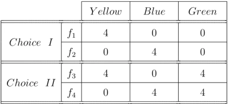
3-color Experiment. There is an urn containing 30 balls, 10 of which are known to be yellow and 20 of which are somehow divided between blue and green, with no further information on the distribution. One ball will be drawn at random from the urn. Subjects face two choice situations,I and II, in which they have to choose between bets paying out 4 or nothing, depending on the color of the randomly drawn ball. In the first choice situation, I, the subjects are asked to choose between two bets: f1, “You

receive 4 if a yellow ball is drawn and nothing otherwise”; and f2, “You receive 4 if a

blue ball is drawn and nothing otherwise”. Similarly, in the second choice situation,II, the subjects have to choose one of two following bets: f3, “You receive 4 if a yellow or

green is drawn and nothing otherwise”; orf4, “You receive 4 if a blue or green is drawn

and nothing otherwise. Table 3.1 summarizes the two relevant choice problems in the 3-color experiment of Ellsberg.

Y ellow Blue Green

Choice I f1 4 0 0

f2 0 4 0

Choice II f3 4 0 4

f4 0 4 4

Table 3.1: Ellsberg’s 3-color experiment

Denote by Y, B and G the event that the ball drawn is yellow, blue and green, respec-tively. For the moment, we describe an event to be unambiguous if its probability is known, i.e. deducible from the available information. Events for which probabilities are unknown are termed to be ambiguous. According to the available information it is natural to assume that subjects view the events Y and B ∪G as unambiguous. The probabilities for their respective occurrence, one third and two thirds, are known. The remaining events are ambiguous. For instance, the probabilities for the event B as well as for the event G are only known to be somewhere between nil and two third. Thus, the observable choices in the 3-color experiment can be viewed as revealing subjects’

(30)

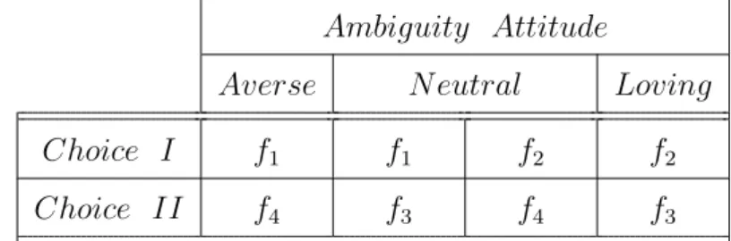
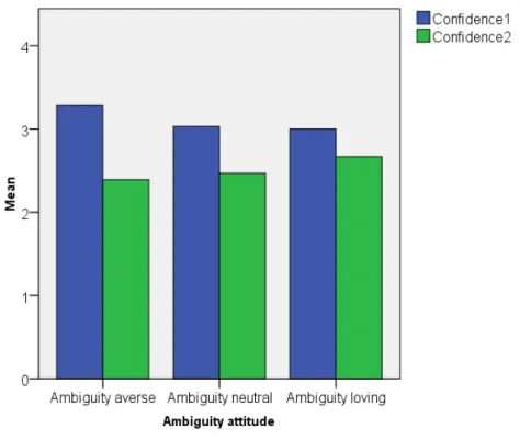
attitudes towards ambiguity. When considering subjects with strong preferences, there are four possible patterns of preferences. Of course subjects can also be indifferent be-tween two alternatives, but then it would not be valid to infer the “ambiguity attitude” from their choices. Each column in Table 3.2 depicts the chosen bet in each of the two relevant choice problems.

Ambiguity Attitude

Averse N eutral Loving Choice I f1 f1 f2 f2 Choice II f4 f3 f4 f3

Table 3.2: Ambiguity attitudes in Ellsberg’s 3-color experiment

The choices depicted in the first and fourth column reflect subjects’ sensitive attitude towards ambiguity. For instance, consider the first column in which the subjects prefer f1 to f2 and f4 to f3. The subjects displaying such preferences are called

ambiguity-averse, since they are reluctant to bet on events with unknown probabilities. Conversely, in the last column, the subjects prefer f2 to f1 and f3 to f4. These subjects are said to exhibit ambiguity-loving behavior, since they favor to bet on events with unknown probabilities.

These two patterns of choices are inconsistent with Savage’s Sure-Thing-Principle. To see this illustrated, consider an ambiguity-averse subject with choices f1 and f4. In the first choice situation, the subject faces two bets f1 and f2 paying off the same amount, 0, if the ball drawn is green. On the other hand, in the second choice situation she faces exactly the same bets labelled f3 and f4, but now with the common payoff of 4 instead of 0 if in the case the ball drawn is green. According to the Sure-Thing-Principle these common payoffs should not affect her choices. Preferences between bets depend only on the payoffs in states in which the payoffs of the two bets being compared are distinct. Thus, if the subject prefers to bet on yellow rather than on blue

(31)

in the first choice situation then she should consequently make the same choices in the second situation. But, this is exactly the logic being violated by the ambiguity-averse subject. She reverses the choices in the second choice situation. One could hypothesize that, the ambiguity-averse subject cannot decide between f3 and f4 without paying attention to the common payoff of these two bets. Then, looking on all states in which the payoff of 4 is possible, she recognizes that bet f3 offers 4 with a probability from the interval between one third and one, whereas bet f4 pays the same amount with the exact probability of one third. Since she does not know which probability is the correct one she decides to choose the betf4 with known probability of getting 4. Thus, the subject exhibiting aversion towards ambiguity violates the separability property inherent in the Sure-Thing-Principle. One explanation for this could be, for instance, that she perceives the events B and G as complementary in the sense that information given on their union cannot be further elaborated.

Moreover, for the ambiguity-averse subject there is no probability distribution that can adequately represent her subjective beliefs. If to the contrary, we assume that she has a subjective probability distribution π, then preferring f1 to f2 implies that she has a higher probability for a yellow ball than for a blue ball to be drawn, i.e. π(Y) > π(B). But, the fact that she prefers f4 tof3 implies that she assigns a higher probability to the event blue or green to be be drawn than to the event yellow or green, i.e. π(Y ∪G) < π(B ∪ G). Thus, by additivity π(Y) < π(B). These two deductions are contradictory. Choices revealing ambiguity-averse behavior violate not only the subjective expected utility theory of Savage, but also any other theory based on probabilistic sophistication in the sense of Machina and Schmeidler (1992, 1995), Grant (1995) or Chew and Sagi (2006, 2008). According to this theory, subjects’ subjective beliefs are represented by a unique and additive probability distribution, but preferences do not need to have expected utility representation.

The second experiment, called 2-color experiment, was originated by Knight (1921). It involves two urns each of them filled with balls of two possible colors.

(32)

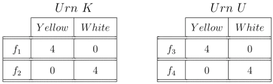
2-color Experiment. There are two urns, K and U, each containing 100 balls. Each ball is either yellow or white. Urn K contains 50 yellow and 50 white balls. In Urn U the proportion of yellow and white balls is unknown. One ball will be drawn at random from each urn. Subjects face four bets paying out 4 or 0, depending on the urn and the color of the ball drawn: f1, “You receive 4 if a yellow ball is drawn from Urn K

and nothing otherwise”; f2, “You receive 4 if a white ball is drawn from Urn K and

nothing otherwise”; f3, “You receive 4if a yellow ball is drawn from Urn U and nothing

otherwise”;f4“You receive4if a white ball is drawn from Urn U and nothing otherwise”.

In the first choice situation, I, subjects are asked for each urn respectively which color do they prefer to bet on. In the second choice situation, II, they are asked for each color respectively which urn do they prefer to bet on. Table 3.3 summarizes the relevant bets in the 2-color experiment.

U rn K

U rn U

Y ellow W hite Y ellow W hite

f1 4 0 f3 4 0

f2 0 4 f4 0 4

Table 3.3: Ellsberg’s 2-color experiment

Denote by YI _and _WI _{the event that a randomly drawn ball from Urn} _I _{∈ {K, U}_} _is yellow and white, respectively. Since the probability for a yellow ball, as well as a white one, to be drawn from Urn K is known to be one half, the events YK and WK are unambiguous. Conversely, the probability for a yellow ball, respectively a white one, to be drawn from Urn U is only known to be in the interval between nil and one. Thus, the eventsYU _and_WU _{and the whole Urn U are purely ambiguous. Again, subjects’ choices} in the 2-color experiment allow us to draw conclusions about their ambiguity attitude. For instance, as Ellsberg observed, a majority of his “non-experimental” subjects are indifferent between betting on yellow and on white when facing Urn K and Urn U, respectively. That is, f1 ∼ f2 and f3 ∼f4. But, when asked whether they prefer that

(33)

prefer the unambiguous Urn U. That is, f1 f3 and f2 f4. Such choices can be seen as revealing aversion towards ambiguity. Moreover, Ellsberg also observed a small minority of subjects who prefer a ball to be drawn form Urn U rather than from Urn K. These subjects seems to be ambiguity-loving. Again, these two pattern of choices violate the Sure-Thing-Principle and they can not be rationalized by a single probability distribution (see Gilboa, 2009, Chapter 12).

Ever since the contribution of Ellsberg there has been overwhelming empirical evi-dence confirming ambiguity-sensitive behavior as a systematic and robust phenomenon. Camerer and Weber (1992) provide a comprehensive survey of the literature on exper-imental studies of decision making under ambiguity. They note a number of stylized facts which emerged from these studies. It is worth mentioning a few of them: “Am-biguity aversion is found consistently in variants of the Ellsberg problems [. . .] (fact 1). Ambiguity aversion persists when preference is strict, excluding indifference (fact 2), and when ambiguity is reduced by drawing samples from ambiguous urns (fact 3). Ambiguity averters have generally not been swayed in experiments that offered writ-ten arguments against their paradoxical choices (fact 4)” (Camerer and Weber, 1992, p.340).

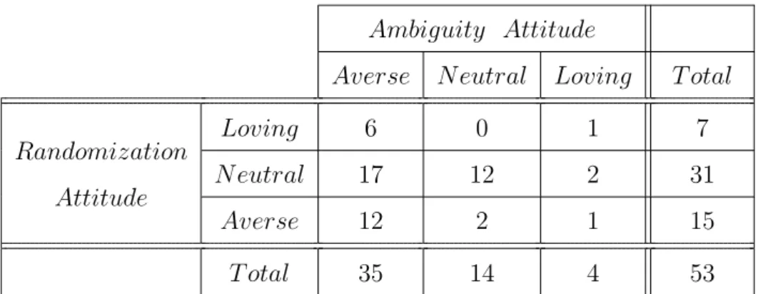
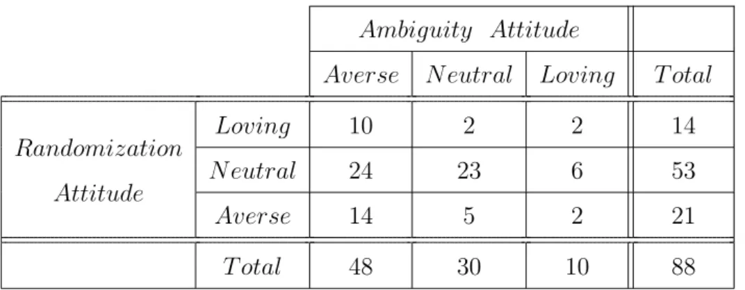
As a part of this thesis we also ran the two experiments inspired by Ellsberg (1961). Our results unequivocally confirm the previous observations. A majority of subjects exhibit ambiguity-sensitive behavior. In the 2-color experiment conducted to examine the relationship between ambiguity and randomization attitudes (see Chapter 4) we observe that: 54.5% of subjects are ambiguity-averse, 11.3% are ambiguity-loving, while 37.5% exhibit neutral attitude towards ambiguity. In the 3-color experiment conducted to test dynamic choice behavior under ambiguity (see Chapter 5) we find a similar pattern: 54.8% of subjects prefer to bet on events with known probabilities, 7.4% prefer to bet on events with unknown probabilities, while 38.1% are ambiguity-neutral. These observations are true for all subjects with strong preferences.

(34)

3.2 Ambiguity Models

In the wake of strong empirical evidence confirming ambiguity-sensitive behavior, sev-eral gensev-eralizations of Savage’s subjective expected utility theory have been suggested. These generalizations seek to provide an alternative representation of preferences apt to explain the Ellsberg-type behavior. The leading idea is to abandon the main tenet of Bayesianism, namely that subjective beliefs are representable by a single probabil-ity distribution. When information about probabilities is too scarce, as in Ellsberg’s experiments, it seems to be more plausible to assume that the decision maker behaves as though she had many possible priors in mind, rather than a single one. There are three widely studied approaches adopting this view. They differ from each other with regard to the notion of subjective beliefs. In the first approach subjective beliefs are represented by a non-additive prior called a capacity, in the second one, by a set of priors called multiple priors and in the third one, by a prior over the set of priors called a second order prior. Note, in these approaches, we discussed below, subjective beliefs are represented uniquely, but not necessarily by a single prior probability distribution.

Non-Additive Prior. Historically, the first axiomatically sound theory of decision making under ambiguity is the Choquet expected utility theory developed by Schmeidler (1989). In this theory subjective beliefs are represented by a capacity. That is, a normalized and monotone, but non-necessarily-additive, set function. The concept of capacity generalizes the notion of probability by weakening the additivity property. The only requirement is that they must satisfy the usual monotonicity property. In other words, the lack of information about likelihoods hinders the decision maker from forming beliefs which satisfy all mathematical properties of probabilities. The decision maker, though, is able to assign weights to uncertain events in such a way that “larger” events (with respect to set inclusion) are “more likely”. By weakening the separability property inherent in Savage’s Sure-Thing-Principle, Schmeidler establish a set of axioms

(35)

which are sufficient and necessary for the existence of a unique capacityνand a unique (up to a positive linear transformation) utility functionu such that for any pair of acts f, g∈ F: f _<g ⇔ Z Ω u(f(ω))dν(ω)≥ Z Ω u(g(ω)) dν(ω). (3.1)

In the presence of non-additive beliefs, expected utilities are computed by means of Choquet integrals, introduced by Gustave Choquet (1954). For this reason this the-ory is called the thethe-ory of Choquet expected utility maximization. In Section 6.1 the notion of capacities and Choquet integrals is defined and discussed in detail. Within the Choquet expected utility theory, the decision maker’s attitude towards ambiguity is mainly captured by the mathematical properties of capacity (see Section 3.3). How-ever, one issue needs to be clarified. How are subjective beliefs, represented uniquely by a capacity, linked to the idea of a non-single prior? Roughly speaking, the tech-nique of Choquet integration provides an answer. The Choquet integral of an act f with respect to the capacity ν can been written as an expected utility with respect to an additive probability measure m. However, the probability measure m depends on the act f being evaluated. More precisely, the measure m depends on how events are ranked with respect to the attractiveness of their outcomes assigned by the act f. In other words, the weight ascribed to an event by m depends not only on the event, but also on how good the outcome yielded by the event under f is in comparison with the outcomes yielded by the other events. In general, two non-comonotonic acts, i.e. acts generating distinct ranking position of mutually exclusive events, will be evaluated with respect to distinct probability measures. Acts generating the same ranking position of states, so-called comonotonic acts, are evaluated with respect to the same probability measure. This is the way in which the independence of beliefs from tastes, the key property of the subjective expected utility theory, is generalized in Schmeidler’s theory. The separability of beliefs from tastes is respected only among comonotonic acts. One could term this property, “comonotonic separability of beliefs from tastes”. For these reasons, the concept of capacities can be seen as a mathematical tool “summarizing”

(36)

all such “rank-dependent” probabilistic scenarios.

Multiple Priors. The second prominent theory known as the maxmin expected utility theory, or “multiple prior” model, was pioneered by Gilboa and Schmeidler (1989). This approach relies on the idea that subjective beliefs are represented by a set C of probability distributions. Intuitively, one can think of each prior in C as describing a possible probabilistic scenario that the decision maker has in mind. With multiple priors in mind the decision maker can still compute expected utility of an act as usual, but now with one expected value per prior. When evaluating the act, the decision maker considers only the probabilistic scenario in which she gets the lowest expected utility. To decide between two acts she compares their lowest expected utilities (which may be obtained with respect to distinct priors) and chooses the one that yields the maximum, among the lowest, expected utility. Gilboa and Schmeidler (1989) provided an axiomatic justification for this decision rule. They established a set of axioms that are necessary and sufficient for the existence of a unique convex and closed set of probability measures C and a unique (up to a positive linear transformation) utility function usuch that for any pair of acts f and g:

f _<g ⇔ min π∈C Z Ω u(f(ω))dπ(ω)≥min π∈C Z Ω u(g(ω))dπ(ω). (3.2)

As in the Savage’s theory, the setCis also purely subjective and represents the decision maker’s perception of ambiguity. WhenC ={π} is a singleton then the decision maker behaves as a subjective expected utility maximizer with a single priorπ. By taking the minimum of the set of all possible expected utility values of an actf the decision maker reveals her reluctance towards ambiguity. The cautious attitude of the decision maker featured by the multiple priors model is often viewed as the result of a malevolent “Na-ture” which can influence the occurrence of events to her disadvantage. That is, Nature chooses a probability π from the set C with the objective of minimizing her expected utilities conditional on her choices. Under this view, Maccheroni, Marinacci, and

(37)

Rus-tichini (2006) extended the multiple prior model by generalizing Nature’s constraint. In their extension, called theory of variational preferences, the constraint on Nature is given by a cost function associated with the choice of a particular probability distri-bution. The cost function is then supposed to capture the decision maker’s attitude towards ambiguity. In other extensions, Ghirardato, Maccheroni, and Marinacci (2004) derive the α-maxmin expected utility representation. In this representation an act is evaluated as a linear combination of maxmin expected utility and maxmax expected utility in which not the worst, but the best expected utility is considered. The maxmin expected utility is weighted with a coefficientα∈[0,1] while the maxmax expected util-ity is weighted with the coefficient 1−α. Both maxmin and maxmax expected utilities are taken with respect to a set of set of priorsC, which is a part of the representation. That is, the set of priorsC and the coefficient αare uniquely defined and may be inter-preted as ambiguity and ambiguity attitude respectively. For instance,α = 1 indicates an extreme aversion towards ambiguity (as in the multiple prior model). By contrast, α = 0 reflects purely ambiguity-loving behavior. Furthermore, modeling α-maxmin preferences in setups with a finite set of states of nature imposes additional restrictions on the parameterα. For such setups, Eichberger, Grant, Kelsey, and Koshevoy (2010) showed that preferences over acts satisfy the axioms of Ghirardato, Maccheroni, and Marinacci (2004) if and only if α = 0 or α = 1. Thus, within finite setups, α-maxmin preferences may only exhibit the two extreme attitudes towards ambiguity.

Second Order Prior. The third approach, proposed by Nau (2006) and further de-veloped by Klibanoff, Marinacci, and Mukerji (2005), is often referred to as the second order prior model, or the smooth ambiguity model. In this approach the decision pro-cess is modeled as a two-stage propro-cess, however, differently than in the tradition of Anscombe and Aumann (1963). A decision maker starts with a set of all probabilistic scenarios captured by the set ∆(Ω).1 _{In addition to it, she comes up with a probability}

1_{That is, ∆(Ω) =}n_p_{: Ω}_→_[0,_1]_|P

ω∈Ωp(ω) = 1 o

(38)

distribution µ over the set of priors, called a second order prior. Intuitively, one can think of the prior µ as describing the probabilistic belief of the decision maker that a particular probabilistic scenario will occur. For instance, consider the set-up of Ells-berg’s 3-color experiment described in Section 3.1. The decision maker may think that the urn has different compositions, each one representing a possible probabilistic sce-nario. Altogether there are twenty-one possible scenarios (from all 20 balls being blue to all 20 balls being green). If the decision maker considers all twenty-one scenarios as possible they will be in the support of her subjective probability distributionµover ∆(Ω). Furthermore, she can distinguish which of the probabilistic scenarios is subjec-tively more likely to occur than the other. The decision process can be summed up as follows. In the first stage a composition of the urn is drawn among a set of hypothetical compositions according to probabilityµ. In the second stage, a ball is drawn from the urn whose composition has been determined by the realisation of µ. Klibanoff, Mari-nacci, and Mukerji (2005) showed that under the seemingly mild assumption imposed on preferences over F, the decision maker choices are characterized by the following decision rule. For any pair of acts f and g,f _<g if and only if:

Z ∆(Ω) φ Z Ω u(f(ω))dp(ω)dµ(p)≥ Z ∆(Ω) φ Z Ω u(g(ω))dp(ω) dµ(p), (3.3)

whereφis function from_Rto_R. The functionφexpresses the decision maker’s attitude towards ambiguity. The evaluation of an act f goes as follows. Once the probabilistic scenario is fixed, the decision maker faces a situation with known probability p and evaluates the act f by its expected utility. Since there are many possible scenarios, the decision maker gets a set of expected utilities off, one for each probabilistic scenario. Then, instead of taking the minimum of these expected utilities, as the multiple priors approach does, an expectation of the function φ distorting the expected utilities is taken. The role of the distortion φ is crucial. If φ is linear then the decision criterion in Equation (3.3) reduces to the expected utility maximization rule with respect to a “reduced” probability distribution obtained by the combination of µ and all possible