Importance Sampling for Coded-Modulation
Error Probability Estimation
Josep Font-Segura,
Member, IEEE,
Alfonso Martinez,
Senior Member, IEEE,
and Albert Guill´en i F`abregas,
Senior Member, IEEE,
Abstract—This paper proposes an efficient simulation method based on importance sampling to estimate the random-coding error probability of coded modulation. The technique is valid for complex-valued modulations over Gaussian channels, channels with memory, and naturally extends to fading channels. The simulation method is built on two nested importance samplers to respectively estimate the pairwise error probability and generate the channel input and output. The effect of the respective number of samples on the overall bias and variance of the estimate of the error probability is characterized. For a memoryless channel, the estimator is shown to be consistent and with a small variance, growing with the square root of the code length, rather than the exponential growth of a standard Monte Carlo estimator.
Index Terms—Coded modulation, random coding, error prob-ability, Monte Carlo simulation, importance sampling.
I. INTRODUCTION
I
MPORTANCE sampling [2], an improved Monte Carlo simulation in which samples are generated according to tilted distributions, may significantly reduce the sampling size in estimating the error probability of a communication scheme [3]. For instance, the transmission of uncoded symbols over the AWGN channel was studied in [4]–[6] with importance sampling techniques, where sampling distributions involve variance scaling and mean translations. Efficient simulation methods of high-performance codes were proposed in, e. g., [7], [8] for low density parity check (LDPC) codes.In this paper, we study the error probability in the detection of coded-modulation signals. Currently, most powerful codes such as polar codes, LDPC codes or turbo codes have large code lengths, an assumption incompatible with the low-latency and ultra-high reliability requirements for next-generation wireless systems. Recently, Polyanskiy, Poor and Verd´u [9] derived tight bounds to the error probability of random codes valid for short code lengths. With random codes, a common tool used in information theory to show the existence of good codes at rates below the channel capacity, one studies the error probability averaged over all possible randomly-generated J. Font-Segura and A. Martinez are with the Department of Information and Communication Technologies, Universitat Pompeu Fabra, Barcelona 08018, Spain; A. Martinez is a Serra H´unter Fellow. (e-mail: {josep.font, alfonso.martinez}@ieee.org).
A. Guill´en i F`abregas is with Instituci´o Catalana de Recerca i Estudis Avanc¸ats, Barcelona 08010, Spain, the Department of Information and Com-munication Technologies, Universitat Pompeu Fabra, Barcelona 08018, Spain, and also with the Department of Engineering, University of Cambridge, Cambridge CB2 1PZ, U.K. (e-mail: [email protected]).
This work has been funded in part by the European Research Council under ERC grant agreement 725411, and by the Spanish Ministry of Economy and Competitiveness under grant TEC2016-78434-C3-1-R.
codes. Evaluating the random-coding error probability, rather than that of a given code, becomes a useful tool to characterize the performance of coded modulation, primarily in channels where good codes are unexplored or unknown. We thus focus on the random coding union (RCU) bound [9, Eq. (62)] to describe the error probability of good codes of arbitrary length. The exact computation of the RCU bound is cumbersome even for short code lengths, as it involves high-dimensional integrations; we address numerical simulation instead. Yet, simulation of such small a quantity would require a number of samples exponential in the code length to achieve an accept-able level of precision [10]. To solve this rare-event simulation problem, we find an importance-sampling tilting that explicitly exploits the known exponential decay of the RCU bound with the code length to estimate the pre-exponential factor of the coded error probability, instead of the full probability.
The rest of the paper is organized as follows. In Sec. II, we describe the error probability of random codes and outline the computational challenges to calculate the RCU bound. We present our efficient importance-sampling simulator of the RCU bound in Sec. III, and derive closed-form expressions of the optimal tilted distributions valid for any block coded modulation. Our estimator consists of two nested importance samplers, respectively related to the estimate of a pairwise error probability and to the generation of the channel input and output. In Sec. IV, we carry out an asymptotic performance analysis for memoryless channels to describe the effect of the number of samples on the overall bias and variance of the nested estimator. We consider some examples with coded binary phase-shift keying (BPSK) modulation over the AWGN and the i.i.d. Rayleigh fading channels in Sec. V, and summarize the main contributions of the paper in Sec. VI.
II. CODED-MODULATIONERRORPROBABILITY LetCbe a block code withM = 2kcodewordsx1, . . . ,xM,
wherekis the number of information bits. Each codewordx has n symbols drawn from a constellation X. The code rate is given by Rb= kn bits per channel use. This code is used for transmission over a channel with conditional probability density Wn(y|x), where the length-n sequence y represents
the equivalent baseband channel output. The error probability, denoted byPe(C), is the probability of decoding in favor of a codeword xj other than the transmitted one xm,j6=m.
The computation of Pe(C)is challenging, due to the com-plex code structure for large values ofn, because of the expo-nentially large number of messages M, or since good codes
themselves are unknown for small n. Instead of considering a fixed codeC, we study the error probabilityPe,naveraged over
all codes ofM codewords generated by independent drawings from some input distributionQn(x). Shannon’s random coding
arguments show the existence of at least one good code whose error probability is at mostPe,n, the expectation ofPe(C)over
all possible codes. Evaluating Pe,n rather than Pe(C) is not
only of theoretical importance but also serves as a performance benchmark for the designers of good codes.
A minor relaxation of the probability Pe,n is given by the
random coding union (RCU) bound to the random coding error probability [9, Eq. (62)], satisfyingPe,n≤rcun, where
rcun=
Z
Qn(x)Wn(y|x) min
1,(M−1)pepn(x,y) dxdy. (1) In (1), the pairwise error probabilitypepn(x,y)is the proba-bility that the decoder decodes in favor of another independent random codeword x for fixed transmitted codeword x and received sequence y, i.e.,
pepn(x,y) =
Z
Qn(x)1{`n(x,y,x)≥0}dx, (2) and1{·}is the indicator function taking the value one if the condition is satisfied and zero otherwise, and `n(x,y,x) is the log-likelihood ratio
`n(x,y,x) = logW n(y|x)
Wn(y|x). (3)
In short, the RCU bound characterizes the error probability of good codes with rateRband lengthn, whose error probability is as good as the right-hand side (r.h.s.) of (1).
The expressions for rcun and pepn(x,y) in (1) and (2)
respectively are both given by an expectation of a non-negative functionf(z)of some random variableZwith densityP(z),
pn= E
f(Z)
, (4)
where from now on we write the expectation operation asE[·]
for the sake of compactness. Evaluating the expectation in (1) involves integrations over joint probability densities
Qn(x)Wn(y|x)Qn(x), (5) which is complex even for simple channels and moderate values ofn. Instead of resorting to approximations (e.g., [11]– [14]), we explore fast and accurate simulation to estimate (1). While the proposed estimator is valid for generic channel law Wn(y|x)and inputQn(x), we restrict our analysis to
mem-oryless channels with product input distributions, for which Wn(y|x) =Qn
i=1W(yi|xi)andQn(x) =Q n
i=1Q(xi).
III. IMPORTANCESAMPLING
The standard Monte Carlo estimate of a quantity pn as
in (4), denoted by pˆn,N, involves generating N samples,
z1, . . . ,zN, according toP(z)and computing the average
ˆ pn,N = 1 N N X i=1 f(zi). (6)
By construction,pn is the mean of each summand in (6). We
also define σ2
n to be the variance, normalized to the squared
mean, of each summand in (6).
In order to describe the accuracy of an estimator in ap-proaching the exact value of the quantity pn as N increases,
we make use of the notion of convergence in probability. Two sequences of random variablesAN andBN indexed byN are
said to converge in probability if for allε >0, it holds
lim
N→∞Pr[|AN −BN|> ε] = 0. (7) We denote the convergence in probability byAN
p −−−−→
N→∞ BN. Using the central limit theorem [15, Ch. XV.5], asN → ∞
the estimatorpˆn converges in probability to ˆ pn,N p −−−−→ N→∞ pn 1 + √σn NΘN , (8)
where and ΘN has a probability density that converges
uni-formly inθto the densitypΘ(θ)of a standard normal random variable Θ. Equivalently, the relative error converges to a normal random variable with zero mean and varianceσ2
n/N, ˆ pn,N−pn pn p −−−−→ N→∞ σn √ NΘ. (9)
The Monte Carlo estimator pˆn,N is unbiased since its
expected value coincides with the quantity to be estimated, namelypn. Besides, whenf(z)in (6) is an indicator function,
using (9) and the fact that the varianceσ2
nis normalized to the
squared mean, i. e.p2
n, we infer that the number of samples
needed to estimate pn to a given confidence level grows as
N ∝p−1
n , [10, Sec. 4.1].
Alternatively, importance sampling is a variance-reducing estimation technique that involves the generation of i.i.d. sam-ples from another distributionP¯(z)[2] to estimatepn as
ˆ pn,N = 1 N N X i=1 ω(zi)f(zi), (10) where the weightsω(z)account for the distribution mismatch and are given byω(z) =P(z)/P¯(z). A good choice forP¯(z)
is known to be the exponential tilting [10]. For anys≥0and a certain functiongn(z), define the tilted distribution
¯
Ps,g(z) =P(z)esgn(z)−κn(s), (11) whereκn(s)is the cumulant generating function [16] ofgn(z), κn(s) = log Eesgn(Z), (12) and the weights are given by
ωs,g(z) =eκn(s)−sgn(z). (13)
Roughy speaking, the importance-sampling estimator ap-proximates the pre-exponential factor αn in the quantity
pn =αn(s)·eκn(s)byαˆn,N, instead of directly estimatingpn.
Hence, the importance-sampling estimator (10) becomes
ˆ pn,N = ˆαn,N(s)·eκn(s), (14) whereαˆn,N(s)is given by ˆ αn,N(s) = 1 N N X i=1 e−sgn(zi)f(z i) (15)
and the samples zi are independently drawn fromP¯s,g(z).
The importance-sampling estimator (14) is unbiased [10, Sec. 4.2] with a normalized sample variance given by
σn2 =E eκn(s)−sgn(Z)f(Z)2 −p2 n p2 n . (16)
The limit in (8) remains valid with a normalized sample vari-ance that is now reduced by properly choosing the parameters s≥0 andgn(z). A good choice ofs is the minimizer of the
cumulant generating function κn(s), i.e., ˆ
sn= arg min s≥0
κn(s). (17)
A. Pairwise Error Probability
For the importance-sampling estimate of the pairwise error probability in (2) with integration variablex, we selectgn(x)
to be the log-likelihood ratio in (3), gn(x) = `n(x,y,x).
As mentioned at the end of this subsection, this choice helps capturing the correct exponential decay of the pairwise error probability in terms ofn for memoryless channels. The corresponding cumulant generating function is given by
κn,τ(x,y) = log E
eτ·`n(x,y,X). (18) For this choice, the tilted distribution P¯τ(x|y)in (11) for the
estimation of pepn(x,y)can be explicitly computed as
¯ Pτn(x|y) = Qn(x)Wn(y|x)τ Z Qn(x0)Wn(y|x0)τdx0 . (19)
While the log-likelihood `n(x,y,x) depends on the channel
input x, this conditional distribution for the codeword x depends only on the channel outputy.
The importance-sampling estimator of the pairwise error probability draws N1 independent samples xj, for j = 1, . . . , N1, from the probability distribution (19) to compute
ˆ γτ,N1(x,y) = 1 N1 N1 X j=1 e−τ·`n(x,y,xj)f pep(x,y,xj), (20) where fpep(x,y,x) =1`n(x,y,x)≥0 , (21) to generate the final estimate
ˆ
pepn,N1(x,y) = ˆγτ,N1(x,y)·e
κn,τ(x,y). (22) Based on (17), we select τ= ˆτn(x,y)given by
ˆ
τn(x,y) = arg min τ≥0
κn,τ(x,y). (23)
Both the optimal parameter τ used in the functionκn,τ(x,y)
and the estimator ˆγτ,N1 depend on x,y. Yet, we henceforth
drop the dependence onx,yinτˆnto lighten the notation. For
the optimal choice ofˆτn, it follows from basic results in
large-deviation theory [17, Th. 2.2.3] that for memoryless channels the pairwise error probability (2) behaves as
lim n→∞
log pepn(x,y)
κn,ˆτn(x,y)
= 1. (24)
B. Random-Coding Error Probability
For the importance-sampling estimate of the random-coding union bound in (1), an expectation with respect to the integra-tion variablesxandy, we choose
gn(x,y) = log(M−1) +κn, 1
1+ρ(x,y), (25) where κn, 1
1+ρ(x,y) is given in (18). We can compute the cumulant generating functionχn(ρ)of gn(x,y)as
χn(ρ) = log E " (M −1)ρ E Wn(Y|X)1+1ρ|Y Wn(Y|X)1+1ρ ρ# . (26) From (11), the distribution used for generating the pair of samples(xi,yi)is given by
¯
Pρn(x,y) =Qn(x) ¯Wρn(y|x), (27) whereW¯ρn(y|x)is a tilted channel transition probability,
¯ Wρn(y|x) = Wn(y|x)1+1ρ E[Wn(y|X)1+1ρ] ρ Z E[Wn(y0|X0)1+1ρ] 1+ρ dy0 . (28)
Equation (27) implies that the channel input sequencesxiare
generated with the original random-coding distributionQn(x)
from Sec. II, whereas the channel output sequences yi are drawn from the modified channel transition probability (28).
Finally, the importance-sampling estimator for the RCU based on the independently generated pairs of samplesxi,yi,
for i= 1, . . . , N2, from the probability distribution (27) is
ˆ rcun,N1,N2= ˆαn,N1,N2(ρ)·e χn(ρ), (29) where ˆ αn,N1,N2(ρ) = 1 N2 N2 X i=1 e−ρ·gn(xi,yi)f rcu(xi,yi) (30) and
frcu(x,y) = min{1,(M−1) ˆpepn,N1(x,y)}. (31)
Based on (17), and taking into account that the cumulant generating function (26) gives the random-coding exponent [18, Sec. 5.6], we selectρas
ˆ
ρn= arg min
0≤ρ≤1
χn(ρ). (32)
For the choice of ρˆn, it follows from basic results in
large-deviation theory [17, Th. 2.2.3] that for memoryless channels
lim n→∞
log rcun
χn( ˆρn) = 1. (33)
The nested importance-sampling estimator is summarized in pseudo-code in Algorithm 1 on the next page. In summary, the channelWn(y|x), the random-coding input distribution of
Qn(x), and the information rateRbjointly determine the outer tilting parameterρˆn, while auxiliary codewords are generated
in accordance to the inner tilting parameter τˆn(x,y) for a given channel input and output pair x,y. As expected, the algorithm extends the classical Monte Carlo method, which can be recovered by settingρˆn= ˆτn= 0.
Algorithm 1: Importance-sampling estimate of the RCU bound Input:Qn(x),Wn(y|x),n,Rb,N2andN1
Output:rcuˆ
calculateM =b2nRbc;
calculateχn(ρ)from (26); selectρ←arg min0≤ρ≤1χn(ρ); findW¯n ρ(y|x)from (28); α←0; fori= 1;i≤N2do generate(xi,yi) according toQ n (x) ¯Wρn(y|x); computeκn,τ(xi,yi)from (18);
selectτ←arg minτ≥0κn,τ(xi,yi); findP¯n τ(x|yi)from (19); γ←0; forj= 1;j≤N1do generatexjaccording toP¯τn(x|yi); γ←γ+N1 1e −τ·`n(xi,yi,xj)1 `n(xi,yi,xj)≥0 ; ˆ pep←γ·eκn,τ(xi,yi); α←α+ 1 N2e −ρ·gn(xi,yi)min{1,(M−1) ˆpep}; ˆ rcu←α·eχn(ρ); returnrcuˆ ;
IV. PERFORMANCEANALYSIS
In the previous section, we presented in Algorithm 1 an importance-sampling estimator for the RCU bound in (1). Built from two nested estimators, the mapping from the general tilting for importance sampling discussed at the beginning of Sec. III was relatively straightforward and led to the respective tilting parametersτˆnandρˆngiven in (23) and (32).
In contrast, the performance analysis is subtler, since the outer estimatorrcun,Nˆ 1,N2is the sum ofN2independent terms
frcu(xi,yi)in (31), each of them a nonlinear function of the
inner estimator pepˆ n,N1(xi,yi). As one estimator is nested
inside the other, a more refined analysis than the central-limit theorem is needed to study the consistency, bias, and variance of Algorithm 1. In this section, we derive an asymptotic expansion of our estimator for memoryless channels and large values ofN1andN2, as summarized in the following theorem.
Theorem. For memoryless channels, as both numbers of samples N1 and N2tend to infinity the importance-sampling estimator of Algorithm 1 converges in probability to the exact RCU bound rcunaccording to
ˆ rcun,N1,N2 p −−−−−−−→ N1,N2→∞ rcun 1− k1,n N1 + r k2,n N2 Θ ! , (34) where k1,n and k2,n are positive numbers growing withn as
O(√n), and Θis the standard normal random variable. The positive term k1,n in (34), linked in Sec. IV-A to
the variance of the estimate of the pairwise error probability
ˆ
pepn,N1(x,y), induces a negative bias in the estimation of the RCU bound. The estimator is asymptotically consistent, as the bias vanishes as N1goes to infinity, although the bias might be significant for small values of N1because its value cannot be reduced by increasing the value of N2. In Sec. V, we numerically validate the expansion in the theorem.
The expression for k2,n in (34) is linked to a significant
reduction in the variance with the importance-sampling
estima-tor, as the number of samples needed to accurately estimate the RCU bound for a given confidence level grows asN2∝
√ n, rather than the typical growthN2∝rcun−1in standard Monte
Carlo [10, Sec. 4.1], which would be exponential behaviour in the code lengthn in our setting of a memoryless channel. Our result (34) is valid under the assumption that
pepn(X,Y) is a strongly non-lattice random variable with a continuous and differentiable density, and that the terms fpep(x,y,X)andfrcu(X,Y)have an integrable characteris-tic function under the joint densities (5). Both assumptions are plausible for the transmission of complex-valued modulations over continuous-output channels considered in this work.
The two remaining subsections are respectively devoted to deriving the biask1,nand variancek2,nterms, and to proving
the asymptotic expansion (34). A. Asymptotic Expansion: Bias
In this subsection, we carry out the asymptotic expansion of the RCU bound estimator (29) up to the term with the factor k1,nin (34) in order to characterize the bias of the estimator.
We start by computing the statistical meanE[ ˆrcun,N1,N2]of
the estimator of the RCU bound (29). For importance-sampling purposes, pairs of channel input and output samples (xi,yi)
are generated according to (27). For the analysis, however, it is more convenient to use the relationship between untilted and tilted probability densities (11) to compute the statistical meanE[ ˆrcun,N1,N2]according to the joint probability density
Qn(x)Wn(y|x). (35) Defining the random variableZ= (X,Y)with densitypZ(z)
in (35), the statistical meanE[ ˆrcun,N1,N2] is given by
E[ ˆrcun,N1,N2] = E
min{1,(M −1) ˆpepn,N1(Z)}
. (36) This quantity does not depend on N2 and depends on N1 through the pairwise error probability estimatorpepˆ n,N
1. We
next expand (36) in a series of inverse powers ofN1. Making use of the observation that for a random variable D and a uniform random variableU in[0,1], it holds that
E[min{1, D}] = Pr[D≥U], (37) we may thus rewrite (36) after taking logarithms in both sides of the inequality inside the probability as
E[ ˆrcun,N1,N2] = Pr
log(M −1) + log ˆpepn,N
1(Z)≥logU
. (38) We continue our analysis by focusing on pepˆ n,N1 for the optimum tilting parameterτˆn(z) in (23). Defining
=√1
N1 (39)
and using (8), it follows that the importance-sampling estima-tor (22) converges as→0to ˆ pepn,N1(z) p −−−−−→ N1→∞ pepn(z) 1 +σpep(z)ΘN1 , (40) where the sample estimation varianceσpep2 (z)is given by
σpep2 (z) =E eκn,ˆτn(z)−τˆn(z)`n(z,X)fpep(z,X) E fpep(z,X) 2 −1, (41)
and the random variable ΘN1 has a conditional density
func-tion pΘN1|Z(θ|z) that converges uniformly to the standard
normal density. The convergence is described by the degree-r Edgeworth expansion [15, Ch. XVI.2]
pΘN1|Z(θ|z) =pΘ(θ)· 1 + r X k=3 k−2Pk(θ,z) ! +o(r−2). (42) In (42), Pk(θ,z) are degree-k polynomials in θ that depend
on the moments of the summation terms in pepˆ n,N1(z)and
on the Hermite polynomials [15, Ch. XVI.1] in θ. These moments are assumed to exist, or equivalently, we assume that the summation terms in pepˆ n,N
1(z) have an integrable
characteristic function under the distribution Qn(x).
Taking logarithms in both sides of (40) and doing a Taylor expansion of order 2 in powers of , we find that
log ˆpepn,N1(z)converges in probability to
log ˆpepn,N1(z)
p −−−−−→
N1→∞
log pepn(z) + Ξn(,z,ΘN1) (43)
since the logarithm is a continuous function, and where
Ξn(,z, θ) =σpep(z)θ−1 2 2 σpep2 (z)θ 2 +O(3). (44) Since the r.h.s. of (38) is a bounded and continuous function ofpepˆ n,N
1(z), the Mann-Wald continuity theorem [15, p. 431]
allows us to substitute (43) into (38). Grouping the summands inside the probability, it proves convenient to define the random variable An(Z, U), sometimes written simply as An
for the sake of compactness, as
An(Z, U) = log(M−1) + log pepn(Z)−logU. (45) With this definition, we find that the statistical mean of the RCU bound estimator converges in probability to
E[ ˆrcun,N1,N2] p −−−−−→ N1→∞ Pr An(Z, U) + Ξn(,Z,ΘN1)≥0 . (46) The random variables AnandΞnhave a joint density
pAn(a)pΞn|An(ξ|a) =pZ(z)pU(u)pΘN1|Z(θ|z). (47) Suppose that pAn(a)is a continuous differentiable density. Under mild assumptions on the joint density of An and Ξn
given in (47), the asymptotic expansion as Ξn vanishes to
zero [19, Th. 1] implies that the r.h.s. of (46) satisfies
Pr[An+ Ξn≥0] = Pr[An≥0] +pAn(0)E[Ξn|An= 0] +1 2p 0 An(0)E[Ξ 2 n|An= 0] +O(Ξ3n). (48) First, notice that using (37) in the first term of the r.h.s. of (48) directly yields the RCU bound in (1), i.e.
Pr
An≥0] = 1−PAn(0) = rcun, (49) wherePAn(a)denotes the cumulative distribution ofAn. We conclude that, as →0 or equivalently N1→ ∞, the RCU bound estimator becomes asymptotically unbiased.
The properties of the Hermite polynomials [15, Ch. XVI.1] imply that
Z ∞ −∞
pΘ(θ)θP3(θ,z) dθ= 0. (50)
Hence, using (50) and the fact that pΘ(θ) is the density of the standard normal random variable, it follows that under the conditional density expansion (42) for r = 3 the remaining expectations in the r.h.s. of (48) are asymptotically given by
E[Ξn|An= 0] =− 1 2 2η n+O(3) (51) and E[Ξ2n|An= 0] =2ηn+O(3), (52) where we defined ηn= E σ2pep(Z)|An= 0 . (53) Noting thatO(Ξ3 n) =O(3)we obtain as→0 that E[ ˆrcun,N1,N2] p −−−−−→ N1→∞ rcun(1−k1,n2), (54)
where the parameterk1,n is given by
k1,n= 1 2ηn pAn(0)−p 0 An(0) 1−PAn(0) . (55)
It remains to characterize asymptotically, as n → ∞, the quantities p0A
n(0), pAn(0), PAn(0), and ηn. For memoryless channels, the variableAnbehaves asymptotically as the sum of
n independent random variables. Standard asymptotic results in the approximation of the density of a strongly non-lattice random variableAn[20, Ch. 2.2] show that asn→ ∞
lim n→∞ pAn(a) ˆ pAn(a) = 1, (56)
wherepˆAn(a)is the saddlepoint approximation to the density of Anata. The saddlepointsˆn is the unique solution to
ˆ
sn= arg min
0≤s≤1
ϕn(s)−sa, (57)
whereϕn(s) is the cumulant generating function of An; the
random variablelogU in (45) limits the region of convergence ofϕn(s)to the[0,1]interval. A similar analysis can be carried out to show that the upper tail probability and the derivative of the density respectively satisfy
lim n→∞ 1−PAn(a) 1 ˆ snpˆAn(a) = 1, (58) and lim n→∞ p0A n(a) −ˆsnpˆAn(a) = 1, (59)
for the same saddlepoint ˆsn in (57). Noting the relationship
in (49) between the random variableAnandrcunand using the
asymptotic equivalence in (33), large-deviation theory results imply that lim n→∞ ϕn(s) χn(s) = 1 (60) and therefore lim n→∞ ˆ sn ˆ ρn = 1. (61)
We recall that ρˆn is the optimal tilting parameter used in the
importance-sampling estimator of the RCU bound. Combining the limits (56), (58) and (59), it follows that
lim n→∞ 1 ˆ ρn(1−ρˆn) pAn(0)−p 0 An(0) 1−PAn(0) = 1. (62)
Since 0 ≤ρˆn≤1 andηn≥ 0, by combining (62) and (55)
we conclude thatk1,nis a non-negative term. For memoryless
channels, the optimal tilting parameter satisfies ρˆn = O(1)
[18, Ch. 5.6]. Therefore, together with (62), we have that pAn(0)−p
0
An(0)
1−PAn(0)
=O(1). (63)
In the last part of this subsection, we study the asymptotics of ηn as n → ∞. This quantity is a conditional expectation
of the sample estimation variance σpep2 (z) given in (41). Noting that E
fpep(z,X)
= pepn(z), we start by studying the asymptotics of pepn(z), whose square appears in the denominator of σ2
pep(z). Refined asymptotic results in the approximation of the tail probability of a sum of strongly non-lattice random variables [20, Eq. (2.2.6)] show that
pepn(z) =√1 ne
κn,ˆτn(z)+O(1) (64) uniformly in z, where κn,τˆn(z) is the cumulant generating function (18) evaluated at the optimal tilting parameter (23). The asymptotics of Efpep(z,X)2 are thus obtained by squaring (64), namely
Efpep(z,X)2= 1
ne
2κn,τnˆ (z)+O(1). (65)
For the remaining terms in σ2
pep(z), we note that the numerator is a tilted tail probability that can be written as
Ωn(z)eκn,ˆτn(z)+κn,−ˆτn(z), (66) whereΩn(z)is a quantity given by
Ωn(z) = Pr
`n(z,X)≥0
(67) and computed under the tilted conditional density
¯
pX|Z(x|z) =Qn(x)e−τˆn(z)`n(z,x)−κn,−ˆτn(z). (68) Letβn(t,z)be the cumulant generating function of`n(z,X)
under the density (68). After some manipulations, we obtain that βn(t,z)is related toκn,τ(z)as
βn(t,z) =κn,t−ˆτn(z)−κn,−τˆn(z). (69) Finding the refined asymptotics for the upper-tail probability
Ωn(z)given by (67) involves computing the unique minimizer
ˆ
tn(z) = arg min t≥0
βn(t,z) (70)
in the region of convergence of βn(t,z), given by [0,∞).
From (69) and (23), it is given by
ˆ
tn(z) = 2ˆτn(z). (71) Therefore, as n→ ∞, we obtain using [20, Eq. (2.2.6)] that
Ωn(z) = √1 ne
κn,τnˆ (z)−κn,−τnˆ (z)+O(1). (72)
Combining (72) with (66), we obtain that the numerator of the pairwise error probability sample variance satisfies
E eκn,ˆτn(z)−τˆn(z)`n(z,X)f pep(z,X) = √1 ne 2κn,τnˆ (z)+O(1). (73)
Using the asymptotic equalities (73) and (65) into (41), we obtain thatσ2
pep(z) =O( √
n)uniformly inz. Sinceηnis the
conditional expectation ofσ2
pep(z)given by (53), we find that ηn=O(
√
n). (74)
Equations (63) and (74) used in the definition of the term k1,n in (55), together with (54), imply that for sufficiently
large code lengthnand number of samplesN1, the expected value ofrcun,Nˆ 1,N2satisfies
E[ ˆrcun,N1,N2] p −−−−−→ N1→∞ rcun 1−k1,n N1 , (75)
wherek1,n is a parameter that grows with nasO(
√ n). This proves the asymptotic expansion (34) asN1→ ∞of the RCU bound estimator (29) up to the term with the factork1,n.
B. Asymptotic Expansion: Variance
In this subsection, we extend the asymptotic expansion of the RCU bound estimator (29) to the term with the factork2,n
in (34) to characterize the variance of the estimator.
To start with, we note that the Lindeberg condition for the central-limit theorem [15, p. 262] is satisfied and that
ˆ
rcun,N1,N2 is given by a sum of N2 independent terms.
Therefore, in an analogous manner to (8), we have
ˆ rcun,N1,N2 p −−−−−→ N2→∞ E[ ˆrcun,N1,N2] 1 + σrcu √ N2 Θ ! , (76) where now from (16) we have
σrcu2 =E eχn( ˆρn)−ρˆngn(Z)f2 rcu(Z) E frcu(Z)2 −1. (77)
As in the previous subsection, we have chosen the optimum tilting parameterρˆnin (32).
We are interested in characterizing the asymptotics of (77) asn→ ∞. We first focus on the numerator in the r.h.s. of (77). Using (31) and thatmin[1, D]2= min[1, D2] forD ≥0, the numerator can be rewritten as
Ψneχn( ˆρn)+χn(−ρˆn), (78) whereΨnis a quantity given by
Ψn= E
min
1,(M−1)2pepˆ n,N1(Z)2 (79) computed under the tilted density
¯
pZ(z) =pZ(z)e−ρˆngn(z)−χn(−ρˆn). (80)
Mimicking the steps followed to derive (46), we use the identityE[min{1, D}] = Pr[D≥U] in (37), take logarithms on both sides of the inequality inside the probability, and substitute the expansion (43) in inverse powers of N1 for
log ˆpepn,N1to show thatΨnconverges in probability as
Ψn p −−−−−→ N1→∞ Pr Bn(Z, U) + Ξn(,Z,ΘN1)≥0 , (81) whereis given in (39),Bnis related toAnin (45) as
and Ξn is given by (44). The tail probability in (81) is
computed under the joint density
¯
pZ(z)pU(u)pΘN1|Z(θ|z), (83)
wherepΘN
1|Z(θ|z)has the Edgeworth expansion (42).
Using the asymptotic expansion from [19, Th. 1], as we did in our analysis of (48), and using again the properties of the Hermite polynomials [15, Ch. XVI.1] in an analogous manner to the steps leading to (51) and (52), we find that as→0
Ψn−−−−−→p
N1→∞
PrBn≥0
+O(2). (84) We next turn our attention to the denominator in the r.h.s. of (77), which we identify as E[ ˆrcun,N1,N2]
2. Taking squares in the expansion in (75) we find that the squared value of
E[ ˆrcun,N1,N2]converges in probability asN1→ ∞torcu
2 nas E[ ˆrcun,N1,N2] 2 p −−−−−→ N1→∞ rcu2n+O( 2 ). (85)
Using (84), (85), and (78) in the formula for σrcu2 in (77), we obtain the asymptotic expansion
σrcu2 −−−−−−−→p N1,N2→∞ k2,n+O(2), (86) wherek2,n is given by k2,n= PrBn≥0 rcu2 n eχn( ˆρn)+χn(−ρˆn)−1. (87) In our next step, we study the asymptotics ofk2,nin (87) as
n→ ∞. We start by studyingrcun, whose square appears in the equation. Refined asymptotic results in the approximation of the tail probability of a sum of strongly non-lattice random variables for non-singular memoryless channels [11, Th. 1] show that the RCU bound (1) satisfies asn→ ∞
rcun= 1
√ ne
χn( ˆρn)−12ρˆnlogn+O(1), (88) whereχn(ρ) andρˆn are respectively given by (26) and (32).
Roughly speaking, equation (88) can be obtained by plugging the refined asymptotics of the pairwise error probability given by (64) into the definition of An in (45), computing the
cumulant generating function of An using the definitions
in (25) and (26), and employing [20, Eq. (2.2.6)] for the tail probability rcun = Pr[An ≥ 0]. The additional term in the
exponent of (88) is the contribution of the √1
n prefactor in (64).
The asymptotics ofrcu2
nare obtained by squaring (88), namely rcu2n= 1
ne
2χn( ˆρn)−ρˆnlogn+O(1). (89)
For the asymptotics of the tail probability PrBn≥0
, we exploit the identity (82) to obtain a similar expansion to (88). To this end, letξn(λ)denote the cumulant generating function of Bn, computed under the joint density (83), and let Ln be
the corresponding region of convergence. Also, letλˆndenote
the optimizer of the cumulant generating function,
ˆ
λn= arg min λ∈Ln
ξn(λ). (90)
The equivalent to (88) for the tail probability Pr[Bn ≥ 0]
involves plugging the refined asymptotics of the pairwise error probability given by (64) into the definitions of An and Bn
in (45) and (82) respectively, and computing the cumulant generating function of Bn under the joint density (83). As
a result, we obtain that
ξn(λ) =χn(2λ−ρˆn)−χn(−ρˆn)−λlogn+O(1). (91)
Similarly to (89), thelognterm in (91) is the contribution of the √1
n prefactor of (64). Using (32), it follows that ˆ
λn= ˆρn+o(1), (92)
where ρˆn is the optimal tilting parameter used in the
importance-sampling estimator of the RCU bound. Using (91) and (92) in [20, Eq. (2.2.6)], we find that
Pr Bn≥0= 1 √ ne χn( ˆρn)−χn(−ρˆn)−ρˆnlogn+O(1). (93)
Finally, substituting (93) back in (87) the resulting expres-sion together with (89), and simplifying the formula, we find thatk2,ngrows withnasO(
√
n). Combining this asymptotics with (86) and (75) into (76), we obtain (34).
V. CODEDBPSK MODULATION
A case of interest is the binary phase-shift keying (BPSK) modulation with symbol set X = {−√P ,+√P}, where P is a positive number describing an average power con-straint. We study the achievable error probability of coded BPSK modulation over both the additive white Gaussian noise (AWGN) and the i.i.d. Rayleigh fading channels. Both cases are examples of continuous-output channels with continuous and differential conditional probability densities for which the required conditions onfpep(x,y,X)andfrcu(X,Y)for the theorem in Sec. IV are satisfied.
A. AWGN Channel
A codeword xis sent over the AWGN channel
y=x+w, (94)
wherewis an i.i.d. real-valued zero-mean Gaussian noise with variance σ2, and we assume perfect synchronization and a coherent receiver. From (94), it follows that
Wn(y|x) = n Y i=1 1 √ 2πσ2e −(yi−xi)2 2σ2 , (95) wherexiandyinow denote theith symbol ofxandy,
respec-tively. Thanks to the symmetry of BPSK, the input distribution Qn(x)that optimizes both the exponential decay (33) and the
channel capacity Cb is the uniform distribution Qn(x) = 1
2n. (96)
For coding ratesRb< Cb, whereCbis the channel capac-ity [18, Eq. (2.2.8)], the RCU bound (1) decays exponentially fast sinceχn( ˆρn)<0 for 0<ρˆn≤1 [18, Eq. (5.6.27)]. For
fixedP andσ2, the coded averageE
b/N0 ratio is defined as Eb N0 = P σ2 · 1 2Rb. (97)
Monte-Carlo evaluation of the RCU bound to the error probability (1) would involve generating triplets (x,y,x)
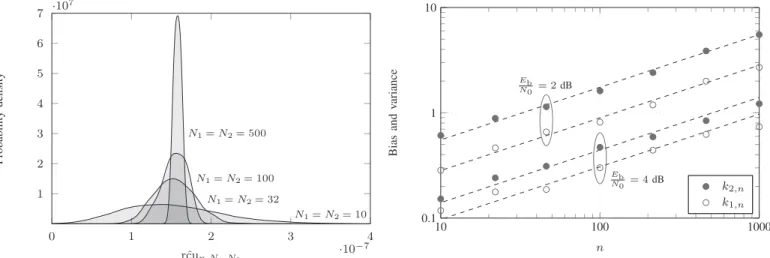
0 1 2 3 4 ·10−7 1 2 3 4 5 6 7 ·10 7 N1=N2= 10 N1=N2= 32 N1=N2= 100 N1=N2= 500 ˆ rcun,N1,N2 Probability density
Fig. 1. Empirical probability density ofrcuˆ n,N1,N2over the AWGN channel,
for code lengthn= 128, code rateRb= 0.5, andEb/N0= 4dB.
according to the joint distributionQn(x)Wn(y|x)Qn(x), and
declaring a decoding error occurs if the codeword x has a higher decoding metric thanx, i.e., ifWn(y|x)≥Wn(y|x).
With importance sampling, we need the distributions
¯
Pτn(x|y) and W¯ρn(y|x). For a given pair of x and y, the
cumulant generating function κτ(x,y)is given from (18) as
κn,τ(x,y) = n X i=1 log e−τ(yi −√P)2 2σ2 +e− τ(yi+√P)2 2σ2 + τ 2σ2 n X i=1 (yi−xi)2−nlog 2. (98)
Hence, the conditional distributionP¯n
τ(x|y)for the estimation
of the pairwise error probability is given from (19) by the following product distribution
¯ Pτn(x|y) = 1 µn,τ(y) n Y i=1 e−τ(yi −xi)2 2σ2 , (99) whereµn,τ(y)is a normalizing factor.
Upon substituting (96) and (95) into (26), the error exponent χn(ρ)is given by (100) at the bottom of the page. As a result, the tilted distribution in (27) involves Qn(x), the distribution
in (96), and the tilted conditional distribution W¯n ρ(y|x) ¯ Wρn(y|x) = 1 µn ρ n Y i=1 e− (yi−xi)2 2(1+ρ)σ2· · e− (yi−√P)2 2(1+ρ)σ2 +e− (yi+√P)2 2(1+ρ)σ2 ρ , (101) with normalizing factor µρ.
Importance sampling for coded BPSK in AWGN chan-nels involves generating codewords with equiprobable BPSK symbols, and generating channel outputs according to the equivalent channel transition probability W¯n
ρ(y|x). Even 10 100 1000 0.1 1 10 Eb N0 = 2dB Eb N0 = 4dB n Bias and v ariance k2,n k1,n
Fig. 2. Empirical biask1,nand variancek2,nterms versusnover the AWGN channel, for code rateRb= 0.5. Dashed lines represent the
√
ninterpolation.
though (101) is not a standard probability distribution, samples can be efficiently generated using the rejection method [21, Ch. II.3]. For a given channel output y, the pairwise error probability is estimated by drawing n BPSK symbols from the binary product distribution (99).
We now proceed to consider several numerical examples. We first fix the code length to n = 128, the rate Rb = 0.5 bits per channel use and the codedEb/N0= 4dB, and show in Fig. 1 a smoothed-kernel density estimation [22] of the importance samplerrcuˆ n,N1,N2for several sampling sizesN1
andN2. We do not consider the Monte Carlo estimation, since it would require at least N2≈109 samples. As we increase bothN1andN2, the both the estimation bias and variance are reduced, in accordance with (34).
To validate the growth of the bias and variance terms of (34) asnincreases, we obtain empirical estimates ofk1,nandk2,n.
For every value ofn, we setN2= 1000, run Algorithm 1 for several values of N1, and find the best interpolated value of k1,nin accordance to (34) neglecting the k2,n term. Fork1,n,
we run the algorithm atN1= 1000andN2= 1several times, compute the sample variance and normalized it according to (34). Fig. 2, plotting k1,n and k2,n against the codeword
length n for a rate Rb = 0.5 bits per channel use at several codedEb/N0 ratios, confirms that both terms grow as√n.
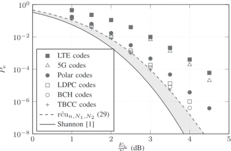
In the remainder in this subsection, we take N1= N2 = 500. As we detailed in Sec. II, the error probability of the optimal code is, at most, the RCU bound. Similarly, using sphere-packing arguments, Shannon established that every code transmitted over the AWGN channel is lower bounded by [1, Eq. (15)]. Therefore, the error probability of good binary codes must lie between the RCU bound and the Shannon lower bound. This region is shaded in gray in the following figures. In Fig. 3, we depict the coded error probability region with high performance codes [23] for code length n = 128, and
χn(ρ) =nρlog(M−1)− n 2 log(2πσ 2) −n(1 +ρ) log 2 +nlog Z ∞ −∞ e− (y−√P)2 2(1+ρ)σ2 +e− (y+√P)2 2(1+ρ)σ2 1+ρ dy (100)
0 1 2 3 4 5 10−8 10−6 10−4 10−2 100 Eb N0 (dB) Pe LTE codes 5G codes Polar codes LDPC codes BCH codes TBCC codes ˆ rcun,N1,N2(29) Shannon [1]
Fig. 3. Error probability versusEb/N0 over the AWGN channel, for code
lengthn= 128, code rateRb= 0.5, andN1=N2= 500samples.
0 200 400 600 800 1,000 10−8 10−6 10−4 10−2 100 Eb N0 = 1dB Eb N0 = 2dB Eb N0 = 3dB n Pe ˆ rcun,N1,N2(29) Shannon [1]
Fig. 4. Error probability versusnover the AWGN channel, for code rate Rb= 0.5,N1=N2= 500samples, and several values ofEb/N0.
rate Rb= 0.5, versus theEb/N0ratio. We include examples of LTE codes (turbo code with 8 states), 5G codes (NR BG 2), polar codes (CRC-7 andL= 32), LDPC codes (F256and OSD t = 4), BCH codes (extended OSD t= 4) and TBCC codes (m= 14). For such a small code length, TBCC codes exhibit good performance, even though there must exist codes with a performance, at most, the RCU bound. Similar conclusions can be obtained from Fig. 4, plotting the coded error probability versus the block length nfor varying Eb/N0.
B. Rayleigh Channel
A second case of interest is the i.i.d. Rayleigh fading channel. For a transmitted codeword x = (x1, . . . , xn) ∈
{−√P ,+√P}n the received sequencey= (y
1, . . . , yn)is
yi=hixi+wi, (102)
where w = (w1, . . . , wn) is an i.i.d. real-valued zero-mean
Gaussian noise with variance σ2, and h = (h
1, . . . , hn) is
i.i.d. Rayleigh distributed with density pn(h) = n Y i=1 2hie−h 2 i1{h i≥0}. (103) SinceE[h2
i] = 1, the coded averageEb/N0ratio remains (97). Assuming perfect channel state information at the receiver (CSIR), the RCU bound to the error probability, averaged over the i.i.d. Rayleigh fading, is given by the expression
rcun=
Z
pn(h)Qn(x)Wn(y|x,h)· ·min
1,(M −1)pepn(x,y,h) dxdydh, (104) where Qn(x) and pn(h) are respectively given by (96) and (103), the channel conditional probability density function Wn(y|x,h)is now given by Wn(y|x,h) = n Y i=1 1 √ 2πσ2e −(yi−hixi)2 2σ2 . (105)
In (104), the pairwise error probability for a fixed transmitted codeword x, received sequence y and fading realization h, denoted aspepn(x,y,h), reads
pepn(x,y,h) =
Z
Qn(x)1{`n(x,y,h,x)≥0}dx (106) for the log-likelihood ratio function
`n(x,y,h,x) = logW
n(y|x,h)
Wn(y|x,h). (107)
The importance-sampling estimator of the RCU bound to the error probability (104) is analogous to the case without fading and involves generating the quadruplet (x,y,x,h)
according to the exponentially-tilted joint distribution pn(h)Qn(x) ¯Wρn(y|x,h) ¯Pτn(x|y,h), (108) with the conditional distribution P¯τn(x|y,h)for the pairwise error probability given by the product distribution
¯ Pτn(x|y,h) = 1 µn,τ(y,h) n Y i=1 e−τ(yi −hixi)2 2σ2 , (109)
whereµn,τ(y,h)is the corresponding normalizing factor, and
¯
Wn
ρ(y|x,h)is the tilted channel conditional distribution ¯ Wρn(y|x,h) = 1 µn ρ n Y i=1 e− (yi−hixi)2 2(1+ρ)σ2 · · e− (yi−hi√P)2 2(1+ρ)σ2 +e− (yi+hi√P)2 2(1+ρ)σ2 ρ (110) with µρ the corresponding normalizing factor. Observe that
the fading realizationhis generated according to the original Rayleigh distribution (103) as, similarly to the case without fading, the exponential tilting of the outer expectation of the RCU (104) only affects the conditional distribution of the received sequencey, while leaving the remaining distributions unaltered. The tilting parameters τ and ρ needed in (109) and (110) are optimally selected as the minimizers
ˆ τn(x,y,h) = arg min τ≥0 κn,τ(x,y,h) (111) and ˆ ρn= arg min 0≤ρ≤1 χn(ρ), (112)
Algorithm 2: Importance-sampling estimate of the RCU bound for BPSK modulation over the i.i.d. Rayleigh fading channel
Input:Qn(x),Wn(y|x),pn(h),n,Rb,N2andN1
Output:rcuˆ
calculateM =b2nRbc;
calculateχn(ρ)from (114); selectρ←arg min0≤ρ≤1χn(ρ); findW¯ρn(y|x,h)from (110); α←0; fori= 1;i≤N2do generate(xi,yi,hi)according to pn(h)Qn(x) ¯Wn ρ(y|x,h); computeκn,τ(xi,yi,hi)from (113); selectτ←arg minτ≥0κn,τ(xi,yi); findP¯τn(x|y,h) from (109); γ←0; forj= 1;j≤N1do generatexjaccording toP¯τn(x|yi,hi); γ←γ+ 1 N1e −τ·`n(xi,yi,hi,xj)1 `n(xi,yi,hi,xj)≥ 0 ; end ˆ pep←γ·eκn,τ(xi,yi,hi); α←α+N1 2e −ρ·gn(xi,yi,hi)min{1,(M−1) ˆpep}; end ˆ rcu←α·eχn(ρ) ; returnrcuˆ ;
where the cumulant generating functions κn,τ(x,y,h) and
χn(ρ) are respectively given as
κn,τ(x,y,h) = n X i=1 log e−τ(yi−hi √ P)2 2σ2 +e− τ(yi+hi√P)2 2σ2 + τ 2σ2 n X i=1 (yi−hixi)2−nlog 2 (113)
and by (114) at the bottom of the page. The nested importance-sampling estimator for the i.i.d. Rayleigh fading channel is summarized in pseudo-code in Algorithm 2 on the top of the page, where by extension we defined
gn(x,y,h) = log(M−1) +κn, 1
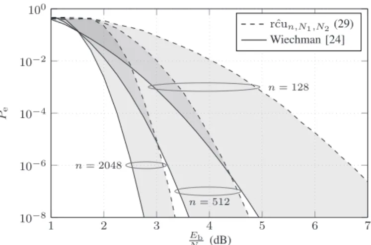
1+ρ(x,y,h). (115) Similarly to the AWGN case, we include an error probability lower bound, the improved sphere-packing bound [24, Th. 3.1] valid for discrete-input continuous-output symmetric channels such as the i.i.d. Rayleigh fading channel described in (102). We take N1=N2= 500to estimate the RCU bound (104) using the importance-sampling Algorithm 2. In Fig. 5, we depict the coded error probability region against the coded Eb/N0 for rate Rb = 0.5, several codeword lengths n. For n = 128, we obtain that RCU bound with i.i.d. Rayleigh fading incurs a 3 dB loss inEb/N0 compared to the AWGN channel in Fig. 3. We also observe that the gap to the error probability lower bound is higher in the presence of i.i.d. Rayleigh fading. By setting n= 1024, we finally show
1 2 3 4 5 6 7 10−8 10−6 10−4 10−2 100 n= 128 n= 512 n= 2048 Eb N0 (dB) Pe ˆ rcun,N1,N2(29) Wiechman [24]
Fig. 5. Error probability versusEb/N0over the i.i.d. Rayleigh channel, for
code rateRb= 0.5,N1=N2= 500samples, and several code lengthsn.
0 1 2 3 4 5 6 7 10−8 10−6 10−4 10−2 100 Rb= 0.25 Rb= 0.5 Rb= 0.75 Eb N0 (dB) Pe ˆ rcun,N1,N2(29) Wiechman [24]
Fig. 6. Error probability versusEb/N0over the i.i.d. Rayleigh channel, for
code lengthn= 1024,N1=N2= 500samples, and several code ratesRb.
in Fig. 2 the coded error probability region against the coded Eb/N0 for several rates above below channel capacity.
VI. CONCLUSION
In this paper, we have presented an importance-sampling technique to estimate the achievable error probability, using random coding arguments, for the transmission of coded data over a continuous-output channel. Exploiting the exponential decay of the error probability, we found closed-form expres-sions for the optimal tilted distributions needed to generate the samples of the two nested estimators involved. We studied the convergence in probability of the estimator and illustrated the transmission of the coded BPSK modulation over the AWGN and i.i.d. Rayleigh fading channels. Our study gives an estimate of the bias and variance of the estimator in terms of the number of samples and the code length, thereby providing guidance on the dimensioning of the nested estimators.
χn(ρ) =nρlog(M−1)− n 2 log(2πσ 2) −n(1 +ρ) log 2 +nlog Z ∞ 0 Z ∞ −∞ 2he−h2 e− (y−h√P)2 2(1+ρ)σ2 +e− (y+h√P)2 2(1+ρ)σ2 1+ρ dydh (114)
REFERENCES
[1] C. Shannon, “Probability of error for optimal codes in a Gaussian channel,”Bell Syst. Tech. Journal, vol. 38, no. 3, pp. 611–656, May 1959.
[2] K. Shanmugam and P. Balaban, “A modified Monte-Carlo simulation technique for the evaluation of error rate in digital communication systems,”IEEE Trans. Commun., vol. 28, no. 11, pp. 1916–1924, Nov. 1980.
[3] B. Davis, “An improved importance sampling method for digital com-munication system simulations,”IEEE Trans. Commun., vol. 34, no. 7, pp. 715–719, Jul. 1986.
[4] D. Lu and K. Yao, “Improved importance sampling technique for efficient simulation of digital communication systems,” IEEE J. Sel. Areas Commun., vol. 6, no. 1, pp. 67–75, Jan. 1988.
[5] R. J. Wolfe, M. C. Jeruchim, and P. M. Hahn, “On optimum and sub-optimum biasing procedures for importance sampling in communication simulation,”IEEE Trans. Commun., vol. 38, no. 5, pp. 639–647, May 1990.
[6] J.-C. Chen, D. Lu, J. S. Sadowsky, and K. Yao, “On importance sampling in digital communications—Part I. Fundamentals,”IEEE J. Sel. Areas Commun., vol. 11, no. 3, pp. 289–299, Apr. 1993.
[7] E. Cavus, C. L. Haymes, and B. Daneshrad, “Low BER performance estimation of LDPC codes via application of importance sampling to trapping sets,”IEEE Trans. Commun., vol. 57, no. 7, pp. 1886–1888, 2009.
[8] S. Ahn, K. Yang, and D. Har, “Evaluation of the low error-rate perfor-mance of LDPC codes over Rayleigh fading channels using importance sampling,”IEEE Trans. Commun., vol. 61, no. 6, pp. 2166–2177, 2013. [9] Y. Polyanskiy, H. V. Poor, and S. Verd´u, “Channel coding rate in the finite blocklength regime,”IEEE Trans. Inf. Theory, vol. 56, no. 5, pp. 2307–2359, May 2010.
[10] J. Bucklew,Introduction to Rare Event Simulation. New York: Springer-Verlag, 2013.
[11] Y. Altu˘g and A. B. Wagner, “Refinement of the random coding bound,”
IEEE Trans. Inf. Theory, vol. 60, no. 10, pp. 6005–6023, 2014.
[12] J. Scarlett, A. Martinez, and A. Guill´en i F`abregas, “Mismatched decoding: Error exponents, second-order rates and saddlepoint approxi-mations,”IEEE Trans. Inf. Theory, vol. 60, no. 5, pp. 2647–2666, 2014. [13] J. Honda, “Exact asymptotics for the random coding error probability,”
inIEEE Int. Symp. on Inf. Theory (ISIT), 2015, pp. 91–95.
[14] J. Font-Segura, G. Vazquez-Vilar, A. Martinez, A. Guill´en i F`abregas, and A. Lancho, “Saddlepoint approximations of lower and upper bounds to the error probability in channel coding,” inConf. on Inf. Science and Sys. (CISS), Princeton, NJ, Mar. 2018.
[15] W. Feller,An Introduction to Probability Theory and its Applications. New York, NY: Wiley, 1971, vol. 2.
[16] R. Durrett,Probability: Theory and Examples. Belmont, CA: Duxbury, 1996.
[17] A. Dembo and O. Zeitouni,Large Deviations Techniques and Applica-tions. Springer Berlin Heidelberg, 2009.
[18] R. G. Gallager,Information Theory and Reliable Communication. John Wiley & Sons, Inc., 1968.
[19] D. R. Cox and N. Reid, “Approximations to noncentral distributions,”
Canadian J. of Stat., vol. 15, no. 2, pp. 105–114, 1987.
[20] J. L. Jensen,Saddlepoint Approximations. Oxford University Press, 1995.
[21] L. Devroye, Non-Uniform Random Variate Generation. New York: Springer-Verlag, 1986.
[22] V. A. Epanechnikov, “Non-parametric estimation of a multivariate prob-ability density,” Theory of Prob. and its Appl., vol. 14, pp. 153–158, 1969.
[23] M. C. Cos¸kun, G. Durisi, T. Jerkovits, G. Liva, W. Ryan, B. Stein, and F. Steiner, “Efficient error-correcting codes in the short blocklength regime,”Phys. Commun., vol. 34, pp. 66–79, 2019.
[24] G. Wiechman and I. Sason, “An improved sphere-packing bound for finite-length codes over symmetric memoryless channels,”IEEE Trans. Inf. Theory, vol. 54, no. 5, pp. 1962–1990, 2008.