DEPARTMENT OF ECONOMICS WORKING PAPER SERIES
Two Stage Semi Parametric Quantile Regression
J. M. Krief
Louisiana State University
Working Paper 2009-05
http://www.bus.lsu.edu/economics/papers/pap09_05.pdf
Department of Economics
Louisiana State University
Baton Rouge, LA 70803-6306
http://www.bus.lsu.edu/economics/
Two Stage Smooth Semi Parametric
Quantile Regression
Jerome Krief
Louisiana State University
∗March 30,2009
Abstract
We propose a root n consistent estimator forβ0when the qth conditional quantile of Y given X=x and Z=z takes the semi linear formg(x) +z0β0whereg(.)is an un-known real valued function,β0 a finite dimensional parameter and (X,Z)a couple of explanatory variables.Importantly, our estimator attains,under homoscedasticity,the semi parametric efficiency bound.This estimation is conducted in two steps. First, a Robinson’s like demeaning of the original model is employed which provides a new quantile regression whose nuisance terms are estimated via a non parametric proce-dure.In the second stage, the quantile regression is conducted by smoothing the check function.We show that the previous estimator belongs to a class of estimators we propose to name ”two stage smooth semi parametric quantile”
JEL-codes: C22, C51. Key words: M-Smoothing,Quantile Regression,Adaptive Esti-mation,Semi Parametric model.
∗Department of Economics,2125 CEBA Bldg., Baton Rouge, LA 70803, phone: (225)
1
Introduction
Quantile regression serves many important purposes in Econometrics. First, even under the Gauss Markov assumptions the LAD (least absolute deviation) estimator minimizing the`1norm of the errors is well acknowledged as a non linear estimator asymptotically more efficient than the OLS ( Koenker and Basset 1978) when the error distribution departs from Normality. Also, conducting a quantile regression permits researchers to obtain a more comprehensive picture of the stochastic relationship between the dependant and the explanatory variables by learning about the ”marginal effects” of the covariates on the various quantiles such as in the field of Labor Economics(Buchinsky 1994).Finally, a valid conditional quantile restriction on the unobservable term of a structural equation permits to identify the parameters of interest due to the equivariance property of the conditionals quantile operator to monotonic transformations, which has proved valuable in the context of censored data (Chen and Khan 2001)and binary choice choice modeling when positing a parametric family for the latent error distribution is untenable1.(Manski 1985,Horowitz 1992)
Similarly to a conditional mean regression, the risk of specification for the conditional quantile is present. Thus, non-parametric point wise estimators for estimating a condi-tional quantile function have been proposed, which essentially extend the kit of kernel based procedures for local mean regression (Watson 1964) to the realm of quantile re-gression(Fan et Al 1994). The local quantile regression (Chaudhuri 1994) is probably the most popular as the asymptotic using the Local Bahadur Representation has been well developed while other approaches seek to improve small sample performance such as spline smoothing (Koeneker 1994), double Kernel smoothing (Yu and Jones 1998) or tackle endogeneity (Horowitz and Lee 2007, Cherozhukov Gagliardini Scaillet 2007).
1The maximum score estimator permits identification of the parameters up to a positive scale, see
Even when asymptotically Gaussien distributed,the above mentioned estimators are not root n consistent with the speed of convergence in probability deteriorating exponentially as the number of explanatory variables increases (often called the ”curse of dimension-ality” in the non parametric jargon). As a reaction to this latter issue, models emerged imposing some form on the multivariate quantile function such as the Additive Quantile Model (Horowitz and Lee 2004) in which case a root n consistent point wise estimator can be constructed via sieves estimation provided the conditional quantile is infinitely smooth.
An interesting sub model is the semi-parametric model for quantile regression, which offers a compromise between efficiency and specification.Lee 2003 is a seminal paper for semi-parametric quantile. First the Average Quantile Estimator(AQR) for the linear part ,under homoscedasticity2,is root n consistent while simultaneously efficient (Newey 1990). Also, under Heteroscedasticity another ”one step” efficient estimator reaching the efficiency bound is proposed.To the best of my knowledge those two estimators are the sole procedures to reach efficiency in the context of a semi parametric quantile regression.
Yet, it is puzzling to notice that the nature of the efficient estimator under homoscedas-ticity,average derivative based(Chaudhuri,Doksum and Samarov 1997), marketably dif-fers from the efficient one under heteroscedasticity, score approximation based(Stone 1975,Bickel 1982).As Econometricians we are familiar with dealing with a class of es-timators for parametric models containing (in the sense of efficiency) a simpler class of estimators such as G.M.M. and Two Stage Least Squares to cite probably the most recognized.This inclusive property is not only theoretically interesting but also it brings guidelines as to what estimator to use in finite sample based upon our testing over the
2Throughout this paper we will employ the same terminology as Lee 2003 for the sake of consistency
keeping in mind that the term homoscedastic error in this context is a substitute forf(0|X, Z) =fε(0)
a.s. wheref(0|X, Z) is the density of the error εconditional on (X, Z) whilefε denotes the marginal
statistical relationship between the unobservable term and the explanatory variables.This last point is all the more relevant in the context of a semi parametric quantile regression because of the complex manner in which the stochastic relationships affect the efficiency bound (see section 6).
In this paper we wish to define a general class of estimators for estimating efficiently the linear part, thus offering a unifying approach to efficient estimation in the context of a semi parametric quantile regression. We introduce this class of estimators we name ”two stage smooth semi parametric quantile”(2SSSPQ)and show that in any stochastic contingency there exists an efficient estimator belonging to this class.The rest of the paper is organized in two parts. In section 2, we rapidly remind the reader about the semi parametric efficiency bound.In section 3-7, we are to focus on the homoscedastic case where the consistency and asymptotic efficiency of a two stage smooth estimator is derived.In section 8,we show that this previous estimator belongs to the 2SSSPQ family whose efficient property for heteroscedastic models are derived generalizing the approach from section 3-7.In section 9, a Monte Carlo experiment illustrates the finite sample properties of a 2SSSPQ.
2
The Semi Parametric Efficiency Bound
In this section we define the efficiency bound for the slope coefficient of a general semi-linear model satisfying for some givenψ(.):
E[ψ(Y −Z0β0−g(X))|X, Z] = 0almost surely (a.s.) where (Y, Z, X) is a R⊗RK ⊗
Rd valued random variable such that (K, d)∈N∗2 and
(β0, g(.))∈RK⊗L2(Rd, µ) is an unknown parameter whereµwill indicate the Lebesgue
measure in the appropriate Euclidean space.Notice that this model is the semilinear conditional mean case(Robinson 1988)when ψ(.) is the identity function while ψ(.) = 1.<0−qfor some q∈(0,1) yields the semilinear conditional quantile model(Lee 2003).
We will note π0(.|x, z)2the Lebesgue density of Y conditional onX =xand Z=zand
Π = {π(.|x, z) ∈L2(R, µ), π(.|x, z)2 >0 and Rπ(.|x, z)2dµ = 1}.The interest is to find
the minimum variance achievable by regular3estimators ofβ0.The concept of an efficiency bound was introduced in Stein 1956 and its the computation for Econometrics models has been typically conducted via the projection method(Bickel 1983,Newey 1990) ,which was successfully employed in Lee 2003 to obtain the efficient bound for a semi parametric conditional quantile model. The next definition is largely adapted from Severini and Tripathi 2001 which provides an alternative to the projection formula in order to obtain the efficient bound. We believe that this approach is more closely linked to the maximum likelihood origin of this concept while additionally often more rapid at retrieving the bound of semi linear models as extensively illustrated in Severini and Tripathi 2001.
Definition
Let suppose thatπ0(.|x, z) belongs toΠ.
Let {πt}t∈[0,b]⊆Πbe an arbitrary curve passing throughπ0 att= 0 for someb >0 and
which is also compatible with the true semi linear conditional model.
Let T(Π, π0) ={π˙ ∈L2(R, µ)a.e.,R ππ˙ 0dµ= 0a.e.} whereπ˙ = ∂π∂tt|t=0.
LetI = 4E[R
˙
π2dµ]be the Maximum Likelihood information for a one parameter problem
and< ., . >z the Fisher inner product on T(Π, π0)inducing the norm||π˙||z=I 1/2.
For any c∈RK letA
c: Π→Rsuch thatAc(πt) =c0βt.Suppose that there exists a linear
functional ∇Ac : (T(Π, π0), < ., . >F)→R such that:
(i)limt→0+|Ac(πt)−tAc(π0)− ∇Ac( ˙π)|=0
(ii)For any {vn}n∈N⊆ T(Π, π0)such thatlimn||vn||z= 0implies limn|∇Ac(vn)|= 0.
3See Newey 1990 and Hajek’s Theorem (1970)for the definition of a regular estimator. This class of
estimators rules out super efficient estimators that may for a family of parametric densities ”beat” the
Then ||∇Ac||2=c0Ω0c for some K by K matrixΩ0, which is called the semi parametric
efficiency bound for regular estimators of β0. Comments:
The efficiency bound is the supremum of the Cramer bound forβ0over all possible para-metric conditional densities that agree with the true density for some one dimensional parameter.Sometimes,this bound is called the Cramer bound of the ”least favorable” model (Stein 1956)because it corresponds to the least efficient Maximum likelihood es-timator of β0.As indicated in the definition,the existence of such bound needs assump-tions.The notion of a curve is the generalization of the Taylor’s representation in Hilbert spaces,which relates to the regularity conditions on the parametric density adopted for ML estimation. In our context {πt}t∈[0,b]⊆Π is a curve passing throughπ0means that for all t ∈[0, b] we have for almost all (x, z)∈Rd⊗RK :
πt=π0+tπ˙+rtfor some rt∈L2(R, µ)suchlimt→0+
R
|rt t|
2dµ= 0.
The curve is said compatible with the true semi linear conditional model when :
R
ψ(y−z0βt−gt(x))π2tdµ= 0 a.e.
so that the functional Ac : Π → R exits, which is needed for deriving the variance of
the maximum ML of β0 under a parametric submodel of density. Once, those later con-ditions hold,the most important requirement is the existence of the pathwise derivative at the true density i.e.π0, which is ensured by (i) and (ii).The intuition behind (i) is that small changes in the parameter of the conditional density around the true value do not abruptly alter the value of the K dimensional parameter of interest. Notice that without(ii)the efficiency bound does not exists so the continuity of the linear functional
∇Ac relates to the existence of regular estimators (Chamberlain 1986),which is an
iden-tification problem.In the semi linear conditional quantile case,(i) and (ii) are satisfied under mild requirement on the density of the error term and the inability to predict Z
from some measurable functions of X.Finally, T(Π, π0) is the linear closure of the ”Cone
Tangent” (Severini and Tripathi 2001),which is our domain of reference for only Cramer bounds of parametric densities satisfying the maximum likelihood score condition are relevant i.e E[∂logπ2t
∂t |t=0] = 0.
We are to succinctly sketch how the efficiency bound is constructed summarizing Severini and Tripathi 2001.In the definition we normalize the true parameter to be 0 for any para-metric family of densities for it does not change the problem. So,letπtbe a curve passing
throughπ0 whent=t0.Since that curve is locally compatible with the semilinear model the functional F such that F πt=βt is well defined. Consequently ˆβM L ,the maximum
likelihood estimator ofβ0, is given byF πˆtM Lwhere ˆtM L=Argmax
ˆ
E[logπ(y|x, z, t)2]
be-cause of the invariance principle of the ML and the assumption of pathwise differtiability of F at ˙π=∂π∂t|t=t0. Hence, there exits a linear functional∇F( ˙π) such that:
F πˆtM L−F πt0 = (ˆtM L−t0)∇F( ˙π) +op(n −1/2) and consequently: asymvar√n( ˆβM L−β0) = Ω( ˙π) where Ω( ˙π) = ∇F( ˙||ππ)˙∇||2F( ˙π)0 z
is just one Cramer bound.Consequentely,any regular estima-tor βR will satisfy for all c inRK:
asymvar√nc0( ˆβR−β0)≥c0Ω( ˙π)c
Since there are possibly an infinity of one parameter problems permitting to recoverer the true conditional densityπ2
0,the supremum ofc0Ω( ˙π)coverT(Π, π0) provides a lower bound for regular estimators.4.Subsequentely,the conclusion of the definition arises because:
4Notice that when any one dimensional parametric model of density returns the same bound, the
c0Ω( ˙π)c= (|c0||∇π˙F||( ˙π)| z )
2
wherec0∇F( ˙π) is what we called∇Ac( ˙π) which is under the previous assumptions (i) and
(ii) well defined as a bounded linear functional on the Hilbert space(T(Π, π0)), < ., . >F)
yielding the efficiency bound as the squared norm of the linear functional.5
3
Motivation for a Robinson’s Like Estimator For Semi
parametric Quantile Regression under
homoscedas-ticity
In this section we introduce the semi linear quantile regression model and rapidly de-scribed the computational steps required from the AQR estimator in order to reach the semi parametric efficiency bound under Homoscedasticity.
The semi parametric quantile regression model posits:
Y =g(X) +Z0β0+ε(I)
P[ε <0|X, Z]=qa.s.for some given q∈(0,1).
where Y is an observable variable,(X, Z) a couple of observable explanatory variables such that (DimX, DimZ) = (d, K) with min(d, K) ≥1 ,g(.) is an unknown function ,β0 a
parameter of interest whileεis the error term.There are essentially two ways to interpret this model. First, the researchers may be primarily interested in estimating theqth
con-ditional quantile function of Y|X, Z positing P[Y < g(X) +Z0β0|X, Z]=q(a.s.)in which case P[ε <0|X, Z]=qa.s. is merely tautological. A good illustration is the conditional
value at risk(R.Engle and S.Manganelli 2005).The second more common interpretation is
5By the Riesz representation theorem there exists a uniqueπ
∗∈T(Π, π0) such that||∇Ac||2=||π∗||2
z
so thatδ= 2(R
that Y is a response variable explained according to some Economic theory whereε con-tains unobservable terms (and/or variables omitted from the underlying theory)andg(.) is left unspecified motivated by the researcher suspicion on the high non-linearity of the relationship between Y and X.This later choice serves two purposes simultaneously.First, it reduces the risk of inconsistent estimation6on the parametric part caused by badly specified g(.), which has been beneficial to testing the relative income hypothesis in Health Economics(A.Jones and J.Wildman 2008).Additionally, relaxing the assumption ong(.) permits to learn more about the relationship between Y and X such as in the field of social learning where the nature of the peer effect can be better uncovered(G.Bobonis and F. Finan 2005).In this instance,P[ε <0|X, Z]=qa.s. is a judiciously chosen
assump-tion on the unobservable component to identify (g(.), β0) among many others constant conditional location restrictions of the formE[Ψ(ε−α)|X, Z] = 0 a.s. for some constant
αand function Ψ(.) satisfying Ψ(.)(.)≥0(Powell 1994).
In a seminal 2003 paper S.Lee showed that the ”Average Quantile Derivative” (AQR) estimator can, under iid sampling, estimateβ0 consistently and efficiently. We are thus to remind the reader briefly about the AQR estimator.For a positive integer k we note
Ak={u ∈ Nd : Pui ≤ k} and Nk its cardinality.Also,for any v ∈ Rd and u ∈ Ak we
use the condensed notation vu for Qd
i=1v
ui
i .Let assume that g(.) is m times
continu-ously differentiable with itsmth derivative also h¨older continuous of exponent γ∈(0,1]
where s=m+γ meets s >3d/2.Given an iid sequence of observations{Yi, Xi, Zi}ni=1
, the efficient AQR estimator is obtained in two steps.In the first stage, this consists of minimizing in c ∈RNk andβ: P i∈Ij,nρq(Yi−Pn(c, Xi, Xj)−Z 0 iβ) forj = 1, . . . , n wherePn(c, t, Xj) =Pu∈Akcuδ −u
n (t−Xj)uis a modified version of the Taylor’s expansion
ofg(.)at some order k aroundXj,Ij,n={i6=j:|Xi−Xj|< δn},δn=O(n−α) for some
α∈(1/2s,1/3d) andρq(t) = (2q−1)t+|t|is the ”check function” (Koenker and Basset
1978).This first stage provides a n-sequence {βˆj}n
j=1, all of which converging in
proba-bility toβ0 at a non parametric rate(Chaudhuri 1991).Hence, the second stage consists of combining this sequence using a judicious weighting system to reach efficiency.Under some mild conditions,βα,the efficient AQR under homoscedasticity is given by:7
βα≡[n1P n
j=1Ω(ˆ Xj)]−1(n1P n
j=1Ω(ˆ Xj) ˆβj)
where ˆΩ(x) is a non parametric estimator ofV ar(Z|X=x).
As showed in Lee 2003, βα has desirable statistical properties in that √
n(βα−β0)
N(0,H) whereHis the efficiency bound, for regular estimators ofβ0under the condition
that the model is homoscedastic.
In the next section, we offer a root nconsistent estimator circumventing the AQR first stage while retaining efficiency.The main conditions we introduce deal with the stochastic relationship between X and the error term and the nature of the random variable X. To be more precise, we impose (i) E[ε|X]=E[ε] a.s. and (ii)X contains either discrete or
continuous bounded variables.Even though assuming statistical independence between X and the error term would suffice for (i) it is generally too strong a condition with economic data.Hence, (i) requiring at least thatεand X be uncorrelated,relaxes the stringency on the degree of stochastic proximity.Finally, it is important to bear in mind that unlike the discrete case ,the bounded support imposes by (ii)does facilitate the derivation of our results but is not necessary when X is a continuously distributed random vector.8
7We removed the X measurable trimming function used in the computation of the AQR,which filters
the sequence of estimators making up the AQR depending on their non parametric part origin,so strictly speaking the efficiency bound is only ”almost” attained because it aims at offering satisfactory finite sample properties.However,as explained in Lee 2003 this has no practical implication asymptotically.
8The intermediate case where X contains a mixture of discrete and continuous variables is possible.The
structure of the proofs being almost identical apart for the more tedious notations we decided not to
4
The Estimation Strategy
Under (i) we can use the operator E[.|X] (Robinson 1988) on both sides of (I) which
yields a new equation and subtracting this latter from (I) results in:
T =w0θ0+ε(II)
where θ00= (−E[ε], β00),T =Y −E[Y|X] and w0= [1,(Z−E[Z|X])0].
We notice that part of the efficient score (Lee 2003)for a semi parametric quantile model emerges in (II),which suggests estimating efficientlyθ0by minimizingPni=1ρq( ˆTi−wˆi0θ)
where the hat stands for non parametric estimates of the nuisance functions. The main issue to overcome pertains to the inevitable first stage estimation of {Ti, wi}ni=1, which
are known up to X measurable nuisance functions we note τ.Let ˆτ be some non para-metric estimator such that plim d(ˆτ , τ)=0 for a pseudo metric d defined on some infi-nite dimensional functional space9containing our functions of interest(Andrews 94)10.In general, showing that the asymptotic will be preserved using preliminary nonparamet-ric estimates demands assumptions.Robinson 1988 succeeded in the context of a semi parametric model for conditional mean, assuming a particular smoothness for g(.) and statistical independence between the error term and (X,Z). Subsequently, Andrews 1994 offered a general sufficient condition with the concept of Stochastic Equicontinuity, which holds under some regularity conditions11.
Yet, the score for a quantile regression is not differentiable.This prevents using Stochastic Equicontinuity as an argument relying on the standard asymptotic theory with the Taylor representation of the score.One solution is provided in the seminal work of Chen et Al
9The term ”pseudo” refers to the fact thatd(f
1, f2) = 0⇔f1=f2almost everywhere. For instance,d
may be induced from a normN(f) = (R
X|f|rdµ)1/r where r is a positive integer and (X,B, µ) some
measure space becaused(f1, f2) =N(f1−f2) satisfies this condition.
10When the support of X is countably finite,the functional space is finite dimensional. However, our
results extend to the case where X is continuous so we adopt a general treatment of the problem.
2003 which,under some regularity conditions, would permit us to derive the asymptotic of the unsmooth feasible estimator relying on the empirical process since this later is path wise differentiable.Even though this last approach could be employed,we rely instead on the smoothing of the objective function because we believe this approach allows for simpler proofs for our specific problem using classic non parametric results for Kernel density estimation.Additionnaly, our approach does not impose to find a pseudo metric satisfying d(ˆτ , τ) = op(n−1/4)(see Chen et Al 2003,Theorem 2-2.4) which is in general
demanding where the dimension of X exceeds the smoothness order of the nuisance functions.
In this paper, we propose to estimateβ0by smoothing the Check function( Amemiya 82, Horowitz 98) minimizing instead:
Pn
i=1ρn( ˆTi−wˆi0θ) (III)
where{ρn}n∈Nis a sequence of twice differentiable real valued functions,converging uni-formly toρq.Those functions are build from integrating kernel functions as to approximate
the absolute value function.The uniform rate of convergence to the check function i.e.sup
|ρn−ρq|will be given by the underlying bandwidthhof the Kernel employed.
The root n consistency and efficiency(under homoscedasticity) of the estimator of β0 based upon (III), which we noteβ(ˆτ), is derived using the following argument.First,using an appropriate smoothing scheme(Horowitz 1998)for the check function will establish that √n(β(τ)−β0) N(0,H) where β(τ) corresponds to the estimator of (III) when
the nuisance parameter is known. Then √n(β(τ)−β(ˆτ)) =op(1) will follow principally
by lettinghvanish as napproaches infinity at a sufficient slow rate, which is decided by the rate of convergence on the nuisance parameters.In other words, our feasible estima-tor from (III)is root n consistent while simultaneously efficiency in the class of regular estimators ofβ0.The logic behind our admissible bandwidth spectrum is intuitive if one
thinks of h as inversely related to the smoothness of the score derived from (III): we need the smoothness of the score to deteriorate slowly enough as to let the estimation mistakes on the nuisance terms have no impact asymptotically.
As explained above, the choice of the bandwidth for smoothing the check function is critical: we must choose h = O(1/np) for some p ∈ (1/2r, c) where r corresponds to
the(uniform)order of smoothness of the density of the error conditional on the explanatory variables and 0< c <1 depends on the nature of X.When X contains discrete random variablesc= 1/4 while a model where X is continuously distributed imposesc=m/4(m+
d) with m > 1 indicating the minimum order of smoothness between the density of X and the nuisance functions.
It is important to stress that the uniform rate of convergence on the nuisance terms plays a pivotal role in deciding the smoothness required on the conditional density for our estimation to be successful. When X comprises discrete random variables,the uniform rate of convergence in probability on the nuisance terms is parametric i.e.√n imposing
r >2 for the density.In the instance where X contains continuous random variables,the (optimal)uniform rate on the nuisance functions isnm/2m+2ddictatingr >2(m+d)/m.
We thus observe two important distinctive features when X contains continuous regres-sors. First, the existence of a trade-off between the smoothness assumption of the nui-sance functions and the error density. Secondly,the presence of a ”linear curse of dimen-sionality in the smoothness” in that the minimal degree of smoothness on the density of the error is increasing in the number of explanatory variables entering g(.)12. In this paper we opted for m= 2 for we wish to be conservative on the class of nuisance func-tions and we believe the cost in terms of r to be very reasonable owing to the small dimensionality of X frequently encountered in semi parametric applications.
12Interestingly, this dimensionality problem attenuates as m becomes large so that the choice for h
becomes identical to the discrete case when the density of X and the nuisance functions are infinitely
Before providing the Model and its full conditions we need to introduce some notations used throughout the paper:
(1)Forr >0 andz∈Rwe noteB(z, r) ={x∈R||x−z|< r}
(2) 1A(x) = 1 , ifx∈A,where A is some real Borel set.
(3) (Ω, σ, P) refers to a probability space where Ω is the space of states of nature,σ is the sigma field of measurable events and P indicates the probability measure.
(4)B= space of real valued Borel measurable functions
(5) For any real valued random variable X and positive integer k we note:
LkX ={f(X), f ∈B,
R
Ω|f(X)|
kdP <∞}, L∞
X the space of X measurable random
vari-ables bounded almost surely and ˆE(f(X)) the plug in estimator ofE(f(X)).
(6) For f:Rd−→
Rwe notef(j)(X) itsjthderivative at X whenever ∂
|j|f(X)
∂xu1 1 ...∂xudd
exists for allu∈Nd such thatPu
i=j.
(7) we note||X||the Euclidean Norm of a vectorX = (x1, ..., xd) and|X|∞=M axi=1...d|xi| where d∈N.
(8) we note |||M|||=√trM0M where M is a finite dimensional real valued Matrix and
M’ its transpose.
(9) we note Xn X forXn converging in distribution to X.
(10) For a joint couple of real valued random variables (A, B) we usefb(a) as the Lebesgue
density of A conditional onB=b.
(11) we use ||L|| for the norm of a linear operator L whenever the context precludes
confusion with the Euclidean norm.
(12)for(d, m)∈N∗2we note:
Φd,m={f : Rd −→ R ,f ∈ B; ||f||sup < ∞(i)R f(X)dX = 1(ii) R Xuf(X)dX = 0 for
[u] = 1, ..., m−1(iii)R
with the standard notationsXu=Qd i=1x ui i foru∈Nd and [u] = P ui.
(13) Form∈NandX ⊂Rd open convex, we noteCm(X)={f :X −→R,f(j) exists and
is continuous forj= 0, ..., muniformly overX }.
(14)we use ||f||∞,X ∗ for the essential supremum of f : Rn −→ R on X ∗ ⊂Rn where
n∈N∗.
For any even integer r greater than 4 we note:
Kr={K : R−→ R, K(t) = Q(t)1[−1,1](t) where Q is a symmetric polynomial of degree r satisfying (i)Q has (r-2)/2 distinct roots in (0,1)(ii)Q(1) = 0;Q(0) > 0 Q(1)(1) =
Q(1)(−1) = 0(iii)R K(t)dt= 1 andR tjK(t)dt= 0 forj= 1, ..., r−1 }.
Fr={ϕ:R−→R,ϕ(u) =Ru∞
R∞
x K(t)dtdx,K∈Kr}.
Finally, for α > 0 and s > 1 we note Hs,α = {f : R −→ R(i)f is r times continously
differentiable wherer−1< s≤r(ii)R
|f(r)(t)|dt <∞}(iii)sup
y∈B(x,%)
|f(y)−Tr−1(y−x)|
|y−x|s ≤
ψ(x) for all x and some % > 0 where Tr−1(y−x) is the Polynomial in the Taylor’s
expansion at order r-1 of f(y) around x (iv)Rfα(x)dx <∞andR
5
The Model
Y =g(X) +Z0β 0+ε Assumption 1: P[ε <0|X, Z]=q a.s. Assumption 2:(a) E|ε|2<∞and (b) E[ε|X]=E[ε] a.s.
Assumption 3:
The support of Z, notedZ, is a compact subset of RK where K≥1.
Assumption 4:
θ00 = (−E[ε], β00) is an interior point of Θ, which is a compact subset ofRK+1.
Assumption 5:
The support of X, noted X, is a countable subset of Rd where d ≥ 1 satisfying (i)
infXP[X=x]>0(ii)Px∈XP[X=x] = 1(iii)inft∈X \x|t−x|>0 uniformly overX.
Assumption 6:
g is a Borel measurable real valued function satisfyingsupx∈X|g(x)|<∞
Assumption 7:
For almost all (x,z)∈ X × Z there existsr(x, z)>0 such thatfx,z(e)>0 on B(0,r(x,z))
where fx,z(.) is the density ofεconditional on X=x and Z=z.
Assumption 8:
Assumption 9:
fx,z(.) is inHr,1 almost everywhere onX × Z.
Assumption 10:
The probability distribution measure of ε is absolutely continuous with respect to the Lebesgue measure.
Comments:
The assumptions follow mostly the literature for linear quantile regression(Koenker and Basset 1978, Amemiya 1982) because our transformed model is in effect linear.We will subsequently elaborate on the assumptions to highlight their relevance in obtaining the re-sults.Nevetheless,it is worth discussing assumptions 2a,4, 5,6 and 9 at this point.Assumption 2a is stronger than usually required where the existence of the first moment of the er-ror suffices. This extra condition originates from the presence of nuisance terms whose rootnconvergence holds provided the central limit theorem applies.Assumption 4 is in-troduced for simplicity but our results remain valid when Θ is simply assumed totally bounded(Andrews 1992),which permits models where strict inequality constraints are imposed on the parameters.Assumption 5,directly taken from Bierens 87,is the defini-tion of a well behaved discrete random variable with (iii) excluding degenerated cases. Assumption 6 is technical but permits along with assumption 2a the convergence of our nuisance terms at the parametric rate(i.e √n).Finally, assumption 9 is a stronger
requirement on the conditional density than proposed in the semi parametric quantile literature(Lee 2003,Chen and Kahn 2001).This type of smoothness requirement on the density is common in the literature of semi parametric estimation based upon prior nui-sance terms(Robinson 1988, Florens et al 2006).That is, just like a classic non parametric density estimation,using a Kernel of orderr >2 demands the density of interest to be r times differentiable. Yet, in this paper we also assume therthderivative of the conditional
density is locally Lipschitz.13.This last modification plays a major role in eliminating the asymptotic bias on the limiting distribution of the smooth quantile estimator.In the re-minding part of the paper we will remove the q subscript for the check function being well understood that the quantile of interest has been chosen i.e. ρ(.) = (2q−1)(.) +|.|
6
Results
Proposition 1 (identification)
Under assumptions 1 through 8
θ0 is the global minimum of E[ρ(T−w0θ)]onΘwhereT =Y −E[Y|X] Comments:
Assumptions 8 and 7 are the most crucial for our parameter of interest to be identi-fied.Assumption 8 requires that Z cannot be perfectly predicted via its minimum MSE predictor on L2X. Thus, this last condition discards models where Z contains a constant
or X measurable functions(power of X for instance)14.This last condition appeared iden-tically in Robinson 1988. Finally, assumption 7 is a classic condition for quantile regres-sion, relevant for unlike mean regression one does not have a globally convex population moment function which prevents the first order condition to suffice.In an Econometrics Model,this condition may be interpreted in terms of the purity of the unobservable com-ponent, which must have some strictly positive probability of getting arbitrary small in absolute term.Using this assumption permits to guarantee that the qth quantile of
the error conditional on X = xand Z = z is unique which, combined to assumption
13This type of condition is useful for dealing with the integrated bias of a kernel density estimator for
a random variable whose support is not compact and can be loosely interpreted as a stability condition on theL1 norm of therthderivative to small perturbation
8, translates into θ0 being the sole local minimum of our population moment and con-sequently the global minimum. It is worth mentioning that the empirical counterpart of E[ρ(T −w0θ)]is not the minimization of interest but the consistency of our smooth estimator(feasible or not) originates from proposition 1.
Proposition 2
let{Ti, w0i}i=1...nbe an iid sequence from a joint couple{T, w0}defined on(Ω, σ, P).For
any q ∈ (0,1) let ρn be a real valued function such that ρn(u) = 2(qu+ϕn(u)) where
ϕn(u) =hϕ(u/h) for some ϕ ∈ Fr and some h = O(1/np) with p ∈ (1/2r,1/4).Then
under assumption 1through 10the followings hold:
(i)θ∗≡ArgminΘP
n
i=1ρn(Ti−wi0θ)is consistent forθ0.
(ii)√n(θ∗−θ0) N(0, q(1−q)E(fx,z(0)ww0)−1E(ww0)E(fx,z(0)ww0)−1).
Comments:
Consequentially, under homoscedasticity this smooth estimator reaches the efficiency bound for the linear part, which is qf(1(0)−q2)E[V(Z|X)]−
1(Lee 2003).The idea of smoothing
M-estimators is not new (Huber 1964)but in the context of a linear quantile regression this consists of mimicking the empirical counterpart for the gradient and Hessian of the pop-ulation function i.e. E[ρ(T−w0θ)],which permits a more rapid derivation of the smooth estimator’s asymptotic because it avoids having to work from a Taylor’s representation of the empirical process (Koenker and Basset 1978).It is important to stress than even though our bandwidth constraint precludes the root nequivalency between this smooth quantile estimator and the minimizer of Pn
i=1ρ(Ti−wi0θ), both estimators’asymptotic
are identical.
The smoothing technique employed in the context of the 2SLAD(Two Stage Least Absolute Deviation)(Amemiya 1982)is simple and analytically tractable since build from
the logistic kernel which is of order 2. Unfortunately, in the context of estimation with nuisance functions one needs a kernel of higher orderr >2 capable of handling bandwidth h such that hr=o(1/√n) to obtain a smooth estimator asymptotically Gaussien and
simultaneously h−4 = o(n) for the nuisance terms to have no impact. Thus, we rely on a variant of Horowitz’s uniform kernel approach(Horowitz 1998) as employed in the context of Bootstrapping. The integration of such kernels of order r is easy to compute and yield polynomials of degree r+ 2 on a compact support which after tuning with a bandwidth approximate the ”check function”. A good example when r = 4 (i.e. for constructing a function in F4) would be the Epanechnikov Kernel given by K(t) = 15/32(7t4−10t2+ 3)1(|t|≤1)resulting inϕ(u) = 15/32(7/30u6−5/6u4+ 3/2u2−16/15u+ 1/6)1(|u|≤1)−u1(u<−1).
Our next step will be to use a modified version of our smooth estimator using non parametric estimates for M(X) =E[Y|X] andϑ(X)=E[Z|X],which we propose to
esti-mate(pointwise) using the following estimators:
ˆ
M(x) =Pn
i=1 ki(x)Yi and ˆϑ(x)=P n
i=1 ki(x)Zi
whereki(x) =φ((Xi−x)/ζ)/Pnj=1φ((Xj−x)/ζ) withφa symmetric Kernel while
ζ is a sequence of bandwidth. We will briefly remind the reader about the conditions upon φleading to our unusual uniform rate of convergence for ˆM and ˆϑby stating the conditions directly taken from Bierens 87.
Proposition 3(Bierens 1987)
let{Yi, Xi, Zi}i=1...n be an iid sequence from (Y, X, Z),a triplet defined on (Ω, σ, P)
where X meets assumption 5. Letφ:Rd −→
Rbe a real valued function satisfying
(i)φis symmetric
(ii)φ(0) = 1
For all x ∈ X let define Mˆ(x) = Pn i=1 ki(x)Yi and ϑˆ(x)=P n i=1 ki(x)Zi where ki(x) =φ((Xi−x)/ζ)/P n j=1φ((Xj−x)/ζ). Thensupx∈X{ √ n( ˆM −M)}=Op(1) andsupx∈X{ √ n||ϑˆ−ϑ||}=Op(1). Comments:
This results originates from the fact that the kernel based estimators converges in probability to the empirical counterpart of the conditional mean which is root n consistent at any point of the conditioning. The condition φ(0) = 1,not typically met by Kernel functions, is at core origin of this convergence success. The intuition is that realizations of X happening to ”hit” the very point of the chosen conditioning x∈ X must ensure
φ((X −x)/ζ)=1 for mimicking the empirical estimator in question. Finally, lim sup
√
n|φ(t)1|t|>1/ζ|= 0 forζ=o(1) is met by Kernels belonging to the exponential family.In practice,φ(.) can be constructed in a simple manner as shown in Bierens 1987 as a linear combination of two normal Kernels:
φ=α1φ1+α2φ2 whereφj(x)=σj−d(2π)−d/2e− x0x/2σ2 j forj= 1,2 αj = (σ−i d−(2π) d/2) σjdσ d i σd j−σdi forj6=i
while{σj}j=1,2 are arbitrary chosen strictly positive real numbers.
Proposition 4
Under assumption 1 through 10
˜
θ∗≡ArgminΘP
n
i=1ρn( ˆTi−wˆi0θ) is consistent for θ0
Assumption 11
For anyδ >0 there existsξ >0 andN0such thatsupn≥N0P[supΘn(ξ)|υn(∆)|> δ]< δ
Comments:
This assumption ensuresυn( ˆ∆) =op(1),which we found to be sufficient to show that
the feasible estimator is asymptotically equivalent. The structure of the condition is inspired from the notion of stochastic equicontinuity (SEC)(Andrews 94).The viability of this assumption may be judged by observing that under our previous assumptions
|υn( ˆ∆)| ≤ √
n|∆ˆ|∞ and is thus bounded in probability15.
Proposition 5
Under assumption 1 through 11
plim|√n(˜θ∗−θ0)−
√
n(θ∗−θ0)|= 0
Comments:
Proposition 5 establishes therefore that our feasible estimator reaches the efficiency bound under homoscedasticity.There are two practical concerns. First, the estimator will be computed minimizing the non linear function Pn
i=1ρn( ˆTi−wˆi0θ) using an iterated
procedure(i.e.Newton’s and its variants)or a direct search method such as simulated annealing(Kirkpatrick et Al 1983).Secondly, to conduct inferences the covariance matrix needs consistent estimators of H0 = E[fx,z(0)ww0] and M0 = E[ww0] which are given respectively by ˆH0 =nh1 Pwˆiwˆ0iK( ˆ Ti−wˆ0iθ˜∗ h ) and ˆM0= 1 n Pwˆ
iwˆi0.16Finally a point wise
estimator of g is given by ˆg= ˆM+ ˆu−ϑˆ0βˆ0 where ˆuis the estimator of the intercept in ˜
θ∗ while ˆβ0its reminding sub vector. Then
√
n(ˆg−g) =Op(1) follows immediately from
propositions 3 and 5.Next we are to provide the conditions for our results to hold in the case where X contains continuously distributed random variables.
15This is no longer true when X has a compact support. 16See Lemma 3 for proof of ˆH
Corollary
Let the previous assumptions of our model hold except assumptions 2a,5,9. Also, let the followings hold:
(a)Xis aX valued random variable whereX ⊂Rd open convex bounded.
(b)X ∗ ⊂ X compact non empty such that{x∈ X ∗|V ar(Z|X =x)positive definite}
has a strictly positive Lebesgue measure.
(c)The distribution function of X is absolutely continuous with respect to the Lebesgue measure and the density of X,noted π,is strictly positive onX.
(d)π,g, andϑbelong toC2(X). (e)E|ε|2+a <∞for some a >0.
(f)There exists constants C1,C2 andC3 such that:
|||E(ZZ0|X=x1)−E(ZZ0|X =x2)||| ≤C1||x1−x2|| for all(x1, x2)∈ X × X.
|E(ε2|X=x1)−E(ε2|X =x2)| ≤C
2||x1−x2|| for all(x1, x2)∈ X × X.
||E(Zε|X =x1)−E(Zε|X =x2)|| ≤C3||x1−x2||for all(x1, x2)∈ X × X. (g)fx,z belongs toHr,1 for almost all(x, z)∈ X × Z withr >2 +d.
The nuisance functions are estimated pointwise with: ˆ M(x)=Pn i=1 ki(x)Yi and ˆϑ(x)=P n i=1 ki(x)Zi whereki(x) =φ((Xi−x)/ζ)/Pnj=1φ((Xj−x)/ζ) (h)φ∈Φd,2 andζ=O(n−1/4+2d). (i)R|R eit0Xφ(X)dX|dt <∞wherei=√−1.
(k)For anyε >0andη >0there existsδ >0such thatlimP∗[supB(τ0,δ) √ n||∇S∗(τ, θ0)− ∇S∗(τ0, θ0)|| > η] < ε where ∇S∗(τ0, θ0) = n1P n i=1 ∂ θρn(Ti−w 0
iθ) |θ=θ0is the true
em-pirical gradient while ∇S∗(τ, θ0) is that using some other nuisance functions τ ∈ F
with F = {(f, g) : ||f||∞,X ∗+||g||∞,X ∗ < ∞},B(τ0, δ) = {τ ∈ F |kF(τ, τ0) < δ} and
kF(τ1, τ2) =||f1−f2||∞,X ∗+||g1−g2||∞,X ∗ for any(τ1, τ2) ={(f1, g1),(f2, g2)} ∈ F ⊗F.
Then θ˜∗ ≡ ArgminΘPni=1λ(Xi)ρn( ˆTi−wˆi0θ),where λ(X) = 1X∈X ∗, satisfies the
followings:
(I) ˜θ∗ is consistent forθ0.
(II)√n(˜θ∗−θ0) N(0, q(1−q)E(λfx,z(0)ww0)−1E(λww0)E(λfx,z(0)ww0)−1).
Comments:
Hence,the semi parametric efficiency bound will be attained under homoscedastic-ity apart for the presence of the trimming function.This ”almost” efficiency is also a characteristics of the efficient AQR when the unobservable term is homoscedastic.It is interesting to notice that while the AQR trimming function has a practical origin(Lee 2003, page7),our trimming criteria is introduced for theoretical reason which are to be explained shortly. In practice one can render the trimming effect inconsequential in large samples by gauging the support of X.Assumption(a)is standard for continuously dis-tributed random variables entering nuisance functions, ensuring a support of ”minimal smoothness”(Andrews 1994).The extra condition we impose is that the support is also bounded,which simplifies many of the proofs but needs not to hold.Assumption (b)ensures thatE[λww0] is positive definite which plays the same role as assumption 8 in the context of our trimmed estimator.This condition is weaker than V(Z|X =x) positive definite
a.e. because it allows Z to be perfectly predicted by X on some strict subsets ofX ∗,which
level of X 17.Assumptionc(c),(d) and (e) ensures the classic conditions to obtain a uni-form rate of convergence in probability on the nuisance functions over compact subsets ofX.Notice that Assumption (d) is conservative on the nuisance functions which comes
at a cost in terms of the smoothness required on the conditional density in (g) where
r > 2 +d is assumed.However,we feel this later condition on the density of the error to be mild as the dimension of the variable entering the non parametric part is small in most economic applications.It is interesting compare the smoothness tradeoff between the AQR and our suggested estimation procedure.Unlike the AQR,it is not the smoothness ofg(.) that must grow with the dimension of X but that of the conditional density of the error term.The bandwidth in (h) for the Kernel employed to estimate the nuisance func-tions is the optimal one under the smoothness condifunc-tions previously enumerated using Kernels of bounded variations(Silverman 1978,Bierens 1987).Assumption (i),required to obtain a uniform rate of convergence in probability on our nuisance functions,demands a Kernel whose Fourier transform is absolutely integrable,which will hold for instance when φ(x)=(2π)−d/2|Σ|−1/2e−1
2x
0Σ−1x
for some positive definite matrix Σ.Finally,the trimming componentλ is introduced because the uniform rate of convergence on con-ditional mean functions is guaranteed only on compact subsets.This filtering of obser-vations has thus been widely used in estimation based upon nuisance functions(Andews 1994,Robinson 1988).Even though trimming imposes a sacrifice in large sample in terms of the efficiency of our estimator,it offers more robust finite sample properties by discard-ing observations close to the cluster points of the support of X.Finally, assumption(k) imposes stochastic equicontinuity (Andrews 94) on the smooth score because assump-tion(d)is not strong enough to ensure the analogue of the discrete case to show directly
√
n{∇S∗(ˆτ , θ0)− ∇S∗(τ0, θ0)}=op(1). TheCaratheodory measure P∗ is introduced in
17For instance,in a simple wage equation usingX =ageand Z=schooling will have the variable
age in a low range as a perfect predictor of schooling as compulsory enrollment prevent any variation to occur for Z.More generally, this type of lack of variation arises with Economic data when some ranges
order to handle instances where supB(τ0,δ)
√
n||∇S∗(τ, θ0)− ∇S∗(τ0, θ0)||is not a σ mea-surable sequence of maps18.Because of our choice for the pseudo metric,this condition can be interpretation as follows: for any τ ∈ F the measure(outer)of the discrepancy
i.e.√n||∇S∗(τ, θ0)− ∇S∗(τ0, θ0)|| exceeding an arbitrary level can be rendered arbitrary small provided that the worst absolute difference overX ∗betweenτ andτ0is kept under
control.Even though (k) is a demanding assumption,it is important to keep in mind that this condition is not necessary to achieve√n{∇S∗(ˆτ , θ0)− ∇S∗(τ0, θ0)}=op(1).
The testing of hypothesis on the slope coefficient will be conducted in practice plug-ging consistent estimators of H0 = E(λfx,z(0)ww0) and M0 = E(λww0) which are given by ˆH0 = nh1 Pλiwˆiwˆi0K( ˆ Ti−wˆi0θ˜∗ h ) and ˆM0 = 1 n P
λiwˆiwˆ0i.Similarly to the
dis-crete case, g(.) will be estimated pointwise as explained on page 22 but with a slower convergence rate imposed by that achieved on the nuisance functions i.e. n2+1d(ˆg −
g) = Op(1).Furthermore, in applications the testing of a null hypothesis of the form
Ho : R∇g(x) = r where ∇g(x) is the gradient of g evaluated at some x ∈ X ,R is
a d by d matric of rank L and r ∈ R may be an object of interest.Under mild
reg-ularity conditions provided in Pagan and Ullah 1999 one can use the fact that that
p
nγd+2(∇gˆ(x)−∇g(x))≡p
nγd+2(∇Eˆ[y−z0β
0|X =x]−∇E[y−z0β0|X =x])+op(1)
to derive under the Null:
p
nγd+2R∇gˆ(x)−r N(0, RΞ(x)R0)
for some Ξ(x) which can estimated consistently non parametrically by nγd+2Ξ(ˆ x),
thus providing a practical testing from (R∇gˆ(x)−r)0(RΞ(ˆ x)R0)−1(R∇ˆg(x)−r) χ2(L).
18P∗ ”measures” a non measurable event A by using measurable coverings of A i.e.P∗(A) =
inf{P
P(Ai)|A⊆ ∪Ai,{Ai} ⊆σ}.In our context,P∗ is useful to show thatE ⊆ BwithE
measur-able andBnon measurable still allows forP(E)≤P∗(B) becauseP∗coincides with P onσ whileP∗
7
Bandwidth selection
We have not addressed so far the selection of the bandwidth for smoothing the check function.Our Monte Carlo experiments suggest that the size of the t-test is highly sensi-tive to the choice of the bandwidth.Even though selection procedures for mean squared error loss have been developed for some M-estimators based upon a smoothing of the density(Horowitz and Hall 1990)the body of research is scant when nuisance functions are present and limited for testing purposes(Gao and Gijbels 2008). Thus, we are to offer a simple rule of thumb based upon the fact that under our assumptions ˆH0 =
HS∗(θ0, τ) +op(1) whereHS∗(θ0, τ) = nh1 Pλiwiw0iK( Ti−w0iθ0
h ) has an asymptotic mean
squared error(componentwise) easy to establish.The following proposition offers an ex-pression for this optimal bandwidth.
proposition 5 bis
LetLbe theK+1byK+1matrix such thatLij=E|HS∗(θ0, τ)ij−E(λfx,z(0)ww0)ij|2
for(i, j)∈ {1, ..., K+ 1}×2. Then under the assumptions of the corollary:
ζ
1 2r+1
0 n
− 1
2r+1 =Argminh|||L|||2as n approaches infinity
where: ζ0= b(1−2r)+√(QB) 4ar a=trace(M2 1);b=trace(M1M2);c=trace(M22) M1= (µrr!)2E[λww0f (r) x,z(0)]22 M2= R K2(t)dtE[λw22w022fx,z(0)] µr= R trK(t)dt
fx,z(r)(0)indicating the rthderivative of the density of εconditional on x, z evaluated
Comments:
Our optimal rate is similar to that minimizing the mean squared integrated error of a Kernel density estimator. However, under assumption (j) of the corollary this optimal bandwidth is not attainable.Yet,this suggests using h∗ =ζ
1 2r+1
0 n−
p for some p meeting
assumption (j). In practice,M1andM2need some consistent estimators for the functions
fx,z(0) andf
(r)
x,z(0) which requires using the feasible version with our residuals to retrieve
ˆ
fx,z(0)and ˆf
(r)
x,z(0) as explained in section 6.Hence, a natural way to proceed in order to
estimate the proposed optimal bandwidth consists of using:
ˆ E[λww0fx,z(r)(0)]22= [n1Pλiwˆiwˆ0ifˆ (r) xi,zi(0)]22 and ˆ E[λw22w220 fx,z(0)] = 1nPλiwˆ22,iwˆ022,ifˆxi,zi(0).
It is yet not clear whether this will provides consistent estimators(under the assump-tions of the corollary)for h* when nuisance funcassump-tions are present because the theory of asymptotic interchangeability between consistent residuals and error terms applies for root-n consistent residuals(Hall and Horowitz 1990) which does not hold under the contin-uous model exposed in the coralary.Thus, one may have to impose assumptions similar to those of section 6 (assumptionH4).Finally, it is important to stress that this optimal cri-teria is merely suggestive because our approximation on the Hessian holds in probability only19and the asymptotic optimal choice may not be relevant in finite sample.However, we believe that this rule of thumb offers a starting point in applications for choosing a range of values for the bandwidth,which is useful should one adopts bootstrapping driven bandwidth selection(Horowitz 1998)or plug in methods(Hall,Sheater,Jones,Marron 1991).
19Hˆ0−HS∗(θ0, τ) =op(1) is not sufficient to conclude that the asymptotic mean squared error of ˆH0 will be equal to that ofHS∗(θ0, τ) because the moments need not to converge unless strong uniform
integrability assumptions are imposed i.e.supnE|||Hˆ0−HS∗(θ0, τ)|||s for somes >2,see Chung page
8
Generalization and discussion
Our paper has introduced an approach to semi parametric quantile regression for estimat-ing efficiently β0, which is generalizable to various stochastic relationships of the triplet (ε, X, Z). In this section the continuous case is treated. For the sake of clarity, it will be convenient to introduce the operator A fromL1(Ω) toL∞
X(Ω) satisfyingAr=E[r|X]
and T from L∞X,Z(Ω) toL∞X(Ω) satisfying T ψ=E[ψ|X](Carrasco,Florens,Renault 2007) whereL∞X,Z(Ω)={Ψ(X, Z),ΨRvalued Borel: ||Ψ(X, Z)||∞<∞ }andL∞X(Ω)={Λ(X),Λ
:Rvalued Borel:||Λ||∞ <∞ }.Given Y =g(X) +Z0β0+ε as the model and using the linearity of A one can show (Newey and Powell 1990)that:
β0 =ArgminβE[f ρ(V −w0β)] (IV) with V =Y −AA(f(f22Y))+ A(f2ε) A(f2) w=Z−AA(f(f22Z))=Z−Γ
where Γ = AA(f(f22Z)) and f indicatesfx,z(0)20.
The demeaning employed in our previous section is therefore transposable to the general case for(IV).Given an iid sequence of observations, one can easily derive that
ˆ
β0 = ArgminβEˆ[f ρ(V −w0β)] (where ˆE denotes the empirical counterpart of (IV))
satisfies:
√
n( ˆβ0−β0) N(0,VB) (V)
whereVB=q(1−q)E[f2ww0]−1is the semi parametric efficiency bound(Lee 2003).This suggests that the parametric part can always be estimated efficiently via a smooth linear quantile regression adjusting for the presence of nuisance terms.
20Our previous model is a special case under what we called homoscedasticity which furnished
Henceforth, we define ˜β∗ = ArgminβEˆ[ ˆf ρn( ˆV −wˆ0β)],the smoothed version of ˆβ0,
as the Adaptive Semi Parametric Quantile Estimator (ASPQ) where τ =(f, g,Γ, β0) is the nuisance parameter, which must be estimated from a first stage. The consistency of
˜
β∗ can be derived from that of ˜θ∗ established in section 5 imposing uniform consistency
conditions on ˆτ =( ˆf ,g,ˆ ˆΓ,βˆ). In practice, both ˆg and ˆβ can be conveniently estimated from the AQR first stage.Also,Γ may be estimated by:
ˆ Γ(X) = Tˆˆ( ˆf2Z) T( ˆf2) ' Pκ(Xi−X cn ) ˆfXi,Zi(0)2Zi Pκ(Xi−X cn ) ˆfXi,Zi(0)2 (V)
for some strictly positiveκ∈Φd,2 andcn=o(1/n) a sequence of bandwidth.
using ˆ fX,Z(0) =hd2+,nKh −(d+K+1) 1,n P κexz(hei1,n, Xi−X h1,n , Zi−Z h1,n) P κxz(Xi −X h2,n , Zi−Z h2,n) (V I)
where {ei}i=1...n are the consistent residuals retrieved from (ˆg,βˆ), (κexz, κxz) ∈
Φd+K+1,2⊗Φd+K,2 while ({h1,n},{h2,n}) are two sequences of bandwidth meeting the
same condition as cn21.
However,the analogy with the Homoscedastic case in terms of the efficiency requires more caution. This arises because the estimator of T(Ψ), where Ψ are the relevant projected elements in Γ, relies on ˆT( ˆΨ)=R ˆ
Ψ ˆfx(z)dz where ˆfx(z) is the non parametric
estimator offx(z) while ˆΨ that of Ψ retrieved from consistent residuals i.e. Y −ˆg−Z0βˆ.
Thus,even though||Tˆ(Ψ)−T(Ψ)||∞ may converges in probability at an acceptable rate
,the same may no longer apply to ||Tˆ( ˆΨ)−T(Ψ)||∞. We are to give next some generic
conditions to ensure consistency and efficiency in this more general setting.
21These suggested feasible versions of non parametric estimators for the nuisance function are the
same as proposed in Lee 2003 to compute the efficient one step estimator under Heteroscedasticity.It is
Assumption H1:
(i)Assumptions 1,3,6,7,10 and (a),(c)of the Corollary hold.
(ii)β0 is an interior point ofB⊂RK compact.
Assumption H2:
(i)X ∗ ⊂ Xcompact non empty such that{x∈ X ∗|E[f2(Z−Γ)(Z−Γ)0|X =x]positive definite}has a strictly positive Lebesgue measure.
(ii)E|ε|<∞
Assumption H3:
There exists (ˆg,βˆ) satisfying:
(i)||ˆg−g||∞=Op(n−γ) for some γ >0
(ii) ˆβ−β0=Op(n−1/2).
Assumption H4:
There existsa >0 andb >0 such that:
(i)supX ×Z|fˆ−f|=Op(n1a)
(ii)||Tˆ−T||=Op(n1b)
Assumption H5:
fx,z(.) belongs toHr,1 for almost all (x, z)∈ X × Z
withr > 1
m wherem=min{a, b, γ}.
Assumption H6:
For anyε >0 andη >0 there existsδ >0 such thatlimP∗[supB(τ0,δ)
√ n||∇S∗(τ, β0)− ∇S∗(τ0, β0)||> η] < ε where ∇S∗(τ0, β0) = ∂β∂ Eˆ[f ρn(Y −g−Γ0β0−(Z−Γ)0β]|β=β0 and ∇S∗(τ, β0) = ∂β∂ Eˆ[ ¯f ρn(Y −g¯−¯Γ 0β¯−(Z−Γ)¯ 0β]|β =β0 for any τ = ( ¯f ,¯g,Γ¯,β¯)∈ F where F = {(f, g, t, b) : f ∈ L∞X ∗⊗Z, g ∈ L∞X ∗, t ∈ ⊗K k=1L∞X ∗, b ∈ RK},B(τ0, δ) = {τ ∈ F |kF(τ, τ0)< δ}andkF(τ1, τ2) =||f1−f2||∞,X ∗⊗Z+||g1−g2||∞,X ∗+supX ∗||t1−t2||+ ||b1−b2||for any (τ1, τ2) ={(f1, g1, t1, b1),(f2, g2, t2, b2)} ∈ F ⊗ F.
Assumption H7:
ρn from proposition 2 is such thath=O(1/np) withp∈(1/2r, m/2).
Assumption H8:
{Yi, Xi, Zi}i=1...nis an i.i.d. sequence from (Y, X, Z).
Proposition 6
Under assumptionH1 throughH8 ˜
β∗≡ArgminBPni=1λifˆiρn(Yi−ˆgi−Γˆ0iβˆ−(Zi−ˆΓi)0β),withλi= 1Xi∈X ∗, is consistent
forβ0 and
√
n( ˜β∗−β0) N(0,VBλ)whereVBλ=q(1−q)E[λf2(Z−Γ)(Z−Γ)0]−1.
Comments:
Identically to the homoscedastic case, the efficiency bound is almost reached be-cause of the trimming term, which can be eliminated if the support of X is assumed to be compact. However, in small sample,it is preferable to retain this filtering of ob-servations as explained on page 25. Assumptions H1 and H2 permit identification of
β0. AssumptionsH3 requires to find some prior estimator of g(.) converging uniformly over X and a root-n estimator of β0. This will be satisfied under the conditions of
the AQR which are provided in Lee 2003 in which case γ = 1/3. Alternatively,there may be other estimators meeting H3 for a semi parametric model if the error term satisfies other scale location invariance restrictions (Robinson 1988,Powel 1994) or spe-cific Heteroscedasticity(section 4).AssumptionsH4, whose sufficient conditions are pro-vided in Bierens 1983 and Horowitz Hall 1990,delivers consistency by ensuring a uniform rate of convergence in probability on the nuisance functions ˆτ =( ˆf ,g,ˆ Γˆ,βˆ).Conditions
H4(ii)refers to||Tˆ−T||=sup||ψ||6=0
||T ψˆ −T ψ||
||ψ|| whose rate of convergence depends on the
”general quality” of the Kernel employed in dealing with the estimation of the projection of (X, Z) measurable elements22.
AssumptionH5 is the familiar smoothness condition on the density of the error term imposed by the uniform of convergence rate in probability achieved on the nuisance functions.Assumption H6 is the stochastic equicontinuity condition, which suffices to ensures the root-n equivalence of the empirical gradients. As in (j) of the Corollary, this seemingly strong assumption it not necessary to obtain this equivalence.
remarks:
(1)It is interesting to compare the one step efficient estimatorβOS proposed in Lee
2003 with the ASPQ.The ASPQ minimizing S(β) = n1Pn
i=1fˆiρn(Yi−ˆgi−Γˆ0iβˆ−(Zi−
ˆ
Γi)0β) has the asymptotic representation:
˜
β∗=β0−HS∗( ¨β,τˆ)−1∇S∗(β0,τˆ) for some ¨β ,wpa.1.
∇S∗(β0,τˆ) = ∂∂βS |β=β0
HS∗( ¨β,τˆ) = ∂
2S
∂ββ0 |β= ¨β.
Conversely the one step efficient estimator suggested in Lee 2003 is computed by:
βOS =bn− {∂∇S∂βn(0β,τˆ) |β=bn} −1∇S n(bn,τˆ),wpa.1. −∇Sn(β,τˆ)∝ n1P n i=1fˆiwˆi [q−Dn(Yi−ˆgi−Zi0β)]
where bn is some available estimator such that √
n(bn−β0) =Op(1) and Dn(.)is a
smooth function whose derivative is a Kernel.Thus,even though the empirical gradient∇Sn
and∇S∗ differ,both estimators are based upon the same principle of approximating the
functiond(.) = 1.<0 with the integral of a Kernel function. That is, both rely on some
differentiableMn(β,τˆ) satisfying :
plim∂Mn(β,τˆ)
∂β0 |β=βn=q(1−q)VB
−1for any consistentβ
and
−√nMn(β0,ˆτ) N(0,[q(1−q)]2VB−1).
which yieldsβef f, the solver of Mn(β,τˆ) = 0 as efficient23.
Hence, unlike the ASPQ,the nature of the one step estimator is approximative because it estimates in finite sample the true representation of its corresponding βef f with the
aid of some root-n consistent estimator.Alternatively, the distinctive nature of the one step may be understood from the perspective of numerical optimization where βef f is
approximated by the Newton’a algorithm using only one iteration and some consistent estimator as the starting value while the ASPQ uses as many iterations as necessary furnishing βef f.
(2)Both estimator can be interpreted as GMM estimators minimizingMn(β,ˆτ)0Mn(β,τˆ)
but the A.S.P.Q. has also(smooth)quantile regression interpreting as the regression ˆf(Y−
ˆ
g−Γˆ0βˆ) on ˆf(Z−Γ).ˆ
(3) In applications,a more expedition way to compute the ASPQ is to notice that ˜
β∗= ˆβ+ ˆδ where ˆδ=ArgminBΣ ˆfiρn(ei−wˆi0δ) where{ei}i=1...n are the residuals from
a first stage.Hence,ˆδcan be interpreted as the efficiency adder.
Identically to the one step estimator,the ASPQ is adaptive in the sense that the semi-parametric efficient bound is always reached.However, there are stochastic relationships for (X, Z, ε) (which can be tested using the AQR first stage residuals)simplifying efficient estimation.To clarify this point letFbe the space of all joint density for(X, Z, ε) meeting the assumptions of our model (2.b excluded) and let H be what we shall name the set of conditions, which is a subset ofR7.We define the ”condition mapping” C as follows:
C:F→H
F7→(||f−f(0)||L1,||f−f(0|X)||L1,||f−f(0|Z)||L1,||µ(X)−µ||L1,||µ(Z)−µ||L1,||µ(X, Z)−
µ||L1,||π(X, Z)−χ(X)ζ(Z)||L1)
whereµ(J)=E[ε|J] for some random variable J,µ=E[ε],χis the marginal density of
X and ζ that of Z.Furthermore,we note {f(h),V(h),W(h)}the random vector from (IV)
when the condition h∈Hholds and{fˆ(h),Vˆ(h),wˆ(h)}its corresponding nonparametric
estimator.For instance, if h contains||f −f(0|X)||L1 = 0 and||µ(X)−µ||L1 >0 we get
f(h) =f(0|X),V(h) =Y −E[Y|X] +E[ε|X] andw(h) =Z−E[Z|X].
Given F0 as the true joint distribution of (X, Z, ε), C(F0) is true set of conditions which we naturally note h0 with its associated efficient bound B(h0).It follows that
ˆ
β(h0) =ArgminβEˆ[ ˆf(h0)ρn{Vˆ(h0)−wˆ(h0)0β}] satisfies
√
n( ˆβ(h0)−β0) N(0, B(h0)).
For instance using our previous example abouth0 a simpler estimator than the ASPQ is the minimizer of ˆE[ ˆfx(0)ρn{Y−Eˆ[Y|X] + ˆE[ε|X]−(Z−Eˆ[Z|X])0β}]which resembles the
estimator covered in section 4-5 apart from the fact that the assumption 2.b no longer holds and that the density weighting approach is employed to reach efficiency (otherwise the estimator would be solely C.A.N.).We define {βˆ(h)|h∈H} as a class of estimators
we name ”two stage smooth semiparametric quantile” given a semi parametric model where ˆβ(h) is efficient forh=h0.
9
Monte Carlo Simulation
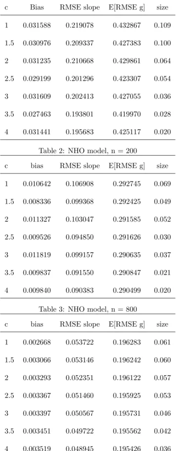
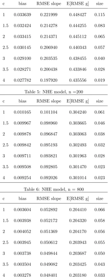
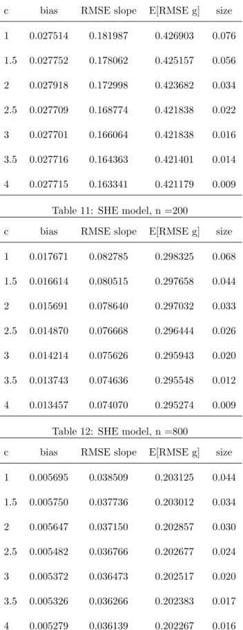
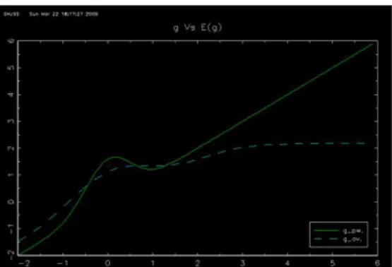
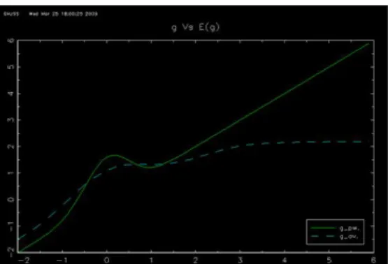
In this section we examine the finite sample properties of the suggested estimator de-scribed in section 6 for the median case(i.e.q=1/2).This estimation strategy is used to estimate the parameterβ= 1 and the functiong(x) =x+√4
2πe
−2x2
(pointwise)when the data generating process obeys:
Y =g(X) +βZ+U
where (X, Z) is a standard bivariate Normal couple of correlation coefficient 0.5.This design was examined in Lee 2003 where g(.) is a bell curve around the origin with the 45 degree line as asymptote.Even though the support of (X, Z) violates assumption 3 and (a) of the corollary the results are not affected The disturbance has the form U=σ where ,independent of (X, Z),is either drawn from a standard normal distri-bution or from a Student distridistri-bution with 4 degrees of freedom (normalized to have a unit variance).We used σ= 1 for the homoscedastic case while σ = eν(X+Z) for the
heteroscedastic model with ν chosen as to normalize the variance of U.We thus exam-ine four designs,the Normal homoscedastic(NHO),the Normal heteroscedastic(NHE), the Student homoscedastic(SHO)and the Student heteroscedastic(SHE).It is rapid to verify that our designs meet assumptions (c) (d) (e) and (f) of the corollary. A simulation of the estimator for a sample size ofn= 50,200 and 800 consists of 1000 replications.The simulations are conducted in Gauss.
The smoothing of the check functions follows proposition 2 and the corollary. We used
ρn(u) =u+2hϕ(u/h) whereϕis (as described on page 15)derived from the Epanechnikov
Kernel of order r = 4, which meets assumption(g)of the corollary owing to the fact that(under the type of distributions adopted for)the smoothness of the density ofU|X, Z
is infinite a.s. A sequence of bandwidth h = O(1/np) with 1/8 < p < 1/6 satisfies
assumption (j). Our preliminary simulations showed that the value of p is immaterial in affecting the results so we decided to use p= 1/7.Hence, our simulations are performed
employing h =cn−1/7with c ∈ {1,1.5,2,2.5,3,3.5,4}.This last range of values for the bandwidth constant is chosen as to containc∗, the optimal values from the perspective of
proposition 5 bis which permits to judge whether,at least locally,the optimal choice put forth in this paper is desirable for inferential purposes. In the model with a normal error we found c∗= 3.086 for the homoscedastic case andc∗ = 2.50 under heteroscedasticity
while the model with a Student error yielded c∗ = 2.62 under homoscedasticity and
c∗= 2.17 for the heteroscedastic case. The estimation of the nuisance functions follows
(h) of the Corollary where the order 2 kernel φ(t) = √1
2πe
−1 2t
2
is employed along with the bandwidth sequence ζ=n−1/6.
Finally, the estimator is computed minimizing by quadratic hill climbing( Goldfeld, Quandt and Trotter 1966)S(θ) =Pn
i=1λ(Xi)ρn( ˆTi−wˆi0θ) whereλ(X) = 1|X|<2is used for the trimming criteria which satisfies assumptions (b) because of the joint normality of (X, Z).Given a n-sample, a search for the global minimum consists of selecting out of 10 iterative searches, the local minimum minimizing S 24as there is no guaranty in
finite sample that the local minimum is unique because the class of Kernel required for smoothing the check function is negative on some intervals.For instance,in our simulation the Kernel of order 4 utilized is strictly negative on (−1,−p
3/7)∪(p3/7,1).
A useful check on whether a local minimum is the global minimum consists of obtain-ing a lower bound B forS on the complement ofP={θ:S:strictly convex}(Demindenko
2000).Let Jn = {i ∈ {1, .., n} : λi = 1} and ˆWJn the #Jn by K+ 1 matrix of
regres-sors excluding observations not in Jn. Let further suppose that the sample at hand is
such that ˆWJnhas full rank.Since ∂2 ∂2θS ∝ P Jnwˆiwˆ 0 iKn( ˆTi−wˆi0θ) whereKn(t) = 1hK(ht) we have P = {θ : Kn( ˆTi−wˆi0θ) > 0∀i ∈ Jn} = {θ : ˆTi−wˆi0θ ∈ Kn−1(0,∞)∀i ∈ Jn} where Kn−1(0,∞) = ∪r2−1
k=1Ok,n and {Ok,n} ⊆ [0,1] are open disjoints intervals which
can be found analytically from the roots of the Kernel on (0,1).Hence,θ ∈ P{ implies 24The different starting values are drawn from a joint N(θ
0,25Id) distribution where Id refers the