Trade Openness, Public Sector Corruption, and Environment: A Panel Data Analysis for Asian Developing Countries

Trade Openness, Public Sector Corruption, and Environment: A Panel Data

Analysis for Asian Developing Countries

Faiza Umer

Corresponding Author is Research fellow at Applied Economics Research Centre (AERC)

University of Karachi and Nielson Karachi- 75270. Pakistan.

Email: [email protected]

Muneeb Khoso

Co Author is Research fellow at Applied Economics Research Centre (AERC)

University of Karachi, Karachi- 75270. Pakistan.

Email:[email protected]

Shaista Alam

Co Author is Assistant Professor at Applied Economics Research Centre (AERC)

University of Karachi,Karachi- 75270. Pakistan.

Email: [email protected] and [email protected]

Abstract

The objective of this present study is to investigate the effect of trade openness and public sector corruption on environment for a panel of 12 developing countries from 1995 to 2012. The study used panel OLS, fixed and random effects models to check the effect of trade openness and public sector corruption on the environment. Government effectiveness used as the measure of public sector corruption. CO2 and methane gas emissions used

as the measure of environmental degradation in this paper. Different specification tests, such as F-test and Hausman specification test are used to make selection among ordinary least square, fixed effect and random effect model. Random effect model seems best to handle such situation.

Keywords:

JEL Classifications:

I. Introduction

During recent years, economists, social scientists and policy analysts have expressed considerable interest in the relationship between trade openness, government effectiveness and the environment. For over a decade’s researchers has been aware of the possible rise in openness to trade which negatively impact on the environmental protection. Most of the earlier empirical literature has focused on the relationship between trade, public sector corruption and the environment which take front position of policy discussions. As abatement cost rises with the stringency of environmental policy regulation has most certainly been a larger factor for making changes in trade liberalization policy and public sector corruption. For instance the analysis about public sector corruption, trade openness and environmental degradation showed that the pressures exerted by globalization can be controlled and reshaped by domestic political institutions1. Advanced industrial countries, do not cut their spending in response to decreasing trade openness. Andonova, Mansfield & Milner (2007), Kaufman & Segura-Ubiergo (2001), Rudra (2002) and Wibbels (2006), has been suggested that trade openness is associated with weaker environmental policy even after government is more effective. Hillman and Ur sprung (1994) estimated the relationships between environmental protection and trade strategies in a model of political corruption. They examined that trade openness policy depends on the nature of the externality, and the environmental preferences are not depend over the global trade. Leidy and Hoekman (1994) discovered the relationship between environmental tools and trade policy, they founds that polluting industries favours inadequate environmental policy because they boosts the level of trade barriers.

The main purpose of this study is to evaluate relationship between trade openness, public sector corruption, and environmental degradation with the help of a panel OLS, fixed and random effect models for panel of twelve Asian countries, i.e. Pakistan, Bangladesh, China, India, Indonesia, Iran, Malaysia, Sri Lanka, Philippines, Thailand, Singapore and Hong Kong. This study is interested in finding other predictions including: (i) trade openness generated by government efficiency (ii) implementation of environmental regulation (iii) output generated by trade openness and (iv) Environment Kuznets curve hypothesis.

This paper differs from previous work in several significant ways. Most notably, and in contrast to existing work, this study deals explicitly with trade openness, public sector corruption and environment. Thus model applies to environmental problems such as CO2 and methane gas emissions, which have previously been ignored in studies. In addition, this study extends the literature by investigating the interaction between government effectiveness and trade openness on policy outcomes. Finally, theoretical model of this study derives testable predictions concerning trade and government effectiveness conversion. The empirical section of the paper tests these predictions by employing panel analysis.

Copeland (1994) investigated the beneficial effects of trade on environmental policy reforms. He also included the case of global factor mobility. Further, the argument to assess globalization and environment is in line with Copeland and Taylor (1995) who analyzes the intentional interaction between developed and poor countries that moves from autarky to free trade, permitting trade-income related environmental policies.

Trade liberalization leads to an increase in the pollution tax if the level of government corruption is high or second is vice versa. On the other hand, if trade policy is not supportive i.e. Import subsidy or export tax is not effective, trade liberalization results in an increase (decrease) in the pollution tax when the degree of corruption is low (high). Antweiler et al., (2001) observed that the effect of trade openness on pollution emissions depend on a country’s comparative advantage. Their study described that trade liberalization always increases the pollution tax due to positive income effect. The main perception about the level of corruption determines the relative importance of bribery versus social welfare. For example, when trade policy is protective and the level of corruption is high, trade liberalization induces a decline in bribery that control second-best welfare considerations. The model by Grossman and Helpman (1994) closely characterizes a form of high-level corruption. Building on the same model, Coate and Morris (1996) also point out that a reduction in corruption unambiguously leads to an increase in the pollution tax. Second is the environmental policy response over corruption is that an increase in the demand for environmental quality is always positive, but disappears and it may negative as the level of corruption increases. In highly corrupt societies, policy formulation is primarily based on bribery, while unorganized countries, entities and groups have little or no influence on environmental policy.

The remainder of the study is organized as follows. Section 2 consists of review of the existing literature. Section 3 outlines the structure of the model and discusses about theoretical framework. Section 4 presents data sources. Section 5 demonstrates the econometric methodology. Section 6 reveals the empirical results, and Section 7 concludes and presents some policy recommendations.

2. Review of Theoretical and Empirical Literature

This section briefly summarizes a few important working papers and articles in the literature looking at the relationship among trade openness, government effectiveness and environment to give some flavor of the literature on the subject. The relationship between trade openness, government effectiveness and environment is a highly debated topic in the environmental growth and development literature. Yet, this issue is far from being resolved. Theoretical studies suggest at best a very complex and ambiguous relationship exist among trade openness government effectiveness and environment. The phenomenal differences among environment condition mostly studies in the South and East Asian, the Latin American, and Sub-Saharan African countries over the last several decades have encouraged a renewed interest in the effects of trade openness and government effectiveness on environmental degradation. The debate on different countries has often been unproductive because they differs greatly in their trust on government actions and typically value the environment differently. It has been disadvantaged by the lack of a common language and also experienced little choices of empirical evidence. The purpose of this study is set out what we currently know about the environmental pollution and international trade with the help of government corruption. The model is developed in Section 3 of the paper and then employed in various appearances throughout. The economic literature on these issues recovered interest stimulated by the policy debates of the past decade.

Much of the earlier literature is focuses on issues like on environmental and international trade issues. Although in general, recent work also focuses on policy analysis but its most significant feature is its concern about how trade openness and public sector corruption affects environmental degradation. This study views these issues as crucial to resolving current policy questions, so most of this study focused on this aspect of the literature.

Strutt and Anderson (2000), reported the case study of Indonesia to 2020, through global economic growth and structural changes they used an extended data set for the periods 1992–2010 and 2010–2020. The conclusions are that trade policy reforms for the next two decades would improve the and reduce the depletion of natural resources, when industrializing country that has more natural resources, devoted to taking part in major national and regional trade liberalizations over the next two decades.

Similar conclusions were reached by Antweiler, Copeland and taylor (2001) by using data for 43 countries over the 1971-1996 period. Their estimates result showed that trade have positive impact on environmental growth. Therefore they conclude free trade is good for environment.

Lopez and Mitra (2000) providing an excellent literature review on the relationship between corruption, income and pollution the Environmental Kuznets Curve (EKC).They investigate the impact of corruption on the empirical relationship between income and pollution the Environmental Kuznets Curve (EKC). They viewed Public sector corruption play a significant role. In general they find evidenced that if Govt. implementing good governance it tend to increase economic growth then it would result to better higher turning point in pollution.

Damania, Fredriksson, and List (2002) have analyzed the case of Organization for Economic Co-operation and Development (OECD) countries using panel random and fixed effect model for the 1982 to 1992 period to examines the causal relationship between corruption trade liberalization and environment. Their results interpreted that, countries with more open trade regimes tend to have stricter environmental regulations on average. Moreover, a reduction in corruption has a greater effect on environmental regulation policy in relatively closed economies. Also they find no robust evidence that the effect of income which is use for the demand for environmental regulation is depending on the level of corruption.

Fredriksson and Svensson (2002) investigated the effect of public sector corruption and political instability on environmental policy by using cross-country data for 63 developed and developing. Their study demonstrated that interaction between corruption and political instability is necessary for environmental policy formation. Their results stress a strong correlation exists between corruption and political instability, and Corruption is significantly negatively correlated with the environmental policies, but corruption effect is reduced when there is higher the degree of political instability.

Managi (2004) using panel data for 63 developed and developing countries for the period from 1960 to 1999 to check whether free trade is harmful or beneficial for the environment. Their study estimated the overall effect of trade liberalization to the environment. He concluded that trade openness is found to have harmful effects on environment.

Frankel and Rose (2002, 2005) contribute to the debate over trade and the environment taking data set of cross-section countries in 1995 to check the impacts of openness to trade on the environment. The main contribution of their paper is to address the endogeneity of income and especially trade, the latter variable drawn from the gravity model of bilateral trade. According to the gravity model, trade is determined by indicators of country size (GDP, population, and land area). They estimate a system of two equations, environmental degradation and economic growth equations. They test the impact of openness on concentrations of NO2, SO2 and Particulate Matter (PM), CO2 emissions, deforestation, energy depletion and rural clean water access when income and other relevant factors held constant. Their results found that trade appears to have a beneficial effect on some measures of environmental quality such as SO2, organic water pollution, and NO2. But their result confirms negative and insignificant relationship exists between trade openness and environment degradation in capital abundant countries.

Copeland and Taylor (2004) examined the environmental consequences of economic growth and international trade by using static model of production-generated pollution. Their debate was originally fueled by North American Free Trade Agreement, the Uruguay round of GATT negotiations and World Trade Organization (WTO). Their result shows that increasing integration of the global economy tends to increase incomes and it has positive impact on domestic environmental policy regulation.

Morse (2007) estimated the relationship between the corruption and Environmental Sustainability in cross-national countries. Their study employed the Environmental Sustainability Index (ESI) taken index for the period 2001, 2002, and 2005, and Corruption Perception Index (CPI) of 2002 created by Transparency International (TI). They find that both CPI and ESI variables were statistically significantly related to income (proxied as GDP per capita). While their research results apparently suggest a significant relationship between corruption, income and environmental degradation.

3. Theoretical Framework and Model Specification

Despite the prevalence of link among trade openness, government effectiveness and environmental degradation, the existing literature in economics has failed to examine the consequences of unique interest of trade liberalization policy on environmental change. This study develops a model in which the trade openness, government effectiveness, some relevant socio-economic variables and interaction terms reveals that how they affect on environment. To this respect cross-country studies evidenced that high public sector corruption have also been related with inequality and low environmental taxes, but there is another debate that poor countries tolerate corruption better than rich countries, (You and Khagram, 2004).

The model of the present study can be described as follows:

Y=F(TO,GE,RGDP,UP,LF,I,YS,K,M,N, E)………...1 Where

Y: Carbon dioxide and Methane gas emissions TO: Ratio of exports plus imports divide by GDP

GE: Government Effectiveness is measure of public sector corruption. Its value lies between +2.5 to -2.5. +2.5 means government is highly efficient, -2.5 means Government is highly corrupted.

RGDP: Real GDP per capita

UP: Urbanization or Urban population (% of total population exposed to industrial pollution/damages) LF: Labor force participation rate (% of total population)

I: Investment (% of total investment in industries)

YS: Years of schooling which indicates education increases income which raises luxurious commodities demand and hence pollution.

K: RGDP2 represents Environmental Kuznets Curve (EKC) hypothesis which described that if income rises, in first stage environmental damages increases but after reaching maximum point income tends to reduces environmental damages as people pay taxes for regulation that’s why Environmental Kuznets curve is inverted ‘U’ shape

Whereas interaction terms are defined as:

M: (TO*RGDP) characterizes as output generated by trade openness N: (GE*RGDP) stands for implementation of environmental regulation

E: (GE*TO) symbolizes as trade openness generated by government efficiency.

4. Data Sources

The time series data on the CO2 and methane gas emission in kilo ton (kt), trade openness (as %), real GDP per capita in constant 2000 US $, investment (as % of total investment in industries), urbanization or urban population (as % of total population exposed to industrial pollution/damages), labor force participation (as % of total population) and enrollment in secondary school collected from the World Development Indicators (WDI: an expanded set of international comparisons, Version-2012). The government effectiveness index is taken from World Governance Indicators. The panel consists of 12 Asian developing countries spanning the years from 1995 to 2012.

5. Econometric Methodology

There are basically three types of panel models namely a pooled Ordinary least square regression, a panel model with fixed effect and panel model with random effect. This study used pooled ordinary least square (OLS), fixed effect model (FEM) and random effect model (REM) for estimation of the effect of trade openness, government effectiveness and all other explanatory variables on carbon dioxide emission and methane gas emissions.

The models are specified as follows:

Yit=όitΩit+µit………..………. (2)

Where Y is the dependent variable (CO2 and methane gas emission), ό represents a vector of explanatory

variables, Ω is slope coefficients, i denotes for the countries t denotes time and µit is the error term which is assumed to be white noised and varies over both country and time. While using a pooled OLS regression, countries’ unobservable individual effects are therefore not controlled. According to Bevan and Danbolt (2004), heterogeneity of the countries under consideration for analysis can influence measurements of the estimated parameters. The fixed-effects model can be derived from equation (2) relative to the notations used in the study as follows:

Yit = αi + λi + β1TOit+ β2GEit + β 3RGDPit + β 4UPit + β 5LFit + β 6Iit + β 7YSit + β 8Kit +β9Mit+β10Nit+β11Eit+ µit………... (3)

In equation (3), Y is the dependent variable (CO2 and methane gas) αi captures unobserved country-specific

effects assumed fixed over time, i –1 dummy variables are used to designate the particular country, this model is sometimes called the least square dummy variables model (LSDV). The dummy for Pakistan is used as comparison country. The year-effects represented by λiare included to account for shocks that are common to all

countries in the sample, year 2012 dummy taken as comparison year in this study. From equation (2) study derives the random-effects model as follows:

Yit = λi + β1TOit γi + β2GEit γi + β 3RGDPit γi + β 4UPit γi + β 5LFit γi + β 6Iit γi + β 7YSit

γi+β8Kitγi+β9Mitγi+β10Nγiti+β11Eitγi+µit,γi= + i ………...….………... (4)

The explanatory variables remain as defined in equation (1). In equation (4) µ is the error term, i represents for

random country effect while is the mean of the coefficient vector. The slope coefficients are allowed to vary randomly across countries, under the random-effects model. Hsiao (1996) argues that the OLS procedure yields biased and inconsistent estimates, especially when the omitted country-specific variables are correlated with the explanatory variables.

This model is a generalized, group-wise heteroscedastic model. For the selection of best model among these models, Ftest and Hausman specification are conducted.

6. Empirical Analysis

This section begins with the empirical analysis by examining the results from the Hausman test with regard to the selection of the most appropriate model between the fixed (FEM) and random effects (REM) frameworks. The Hausman test statistics presented in Table 1 and 3 indicate that the random effect model should be preferred over the fixed effect model. In each model (1-8), the test statistic suggests that the null hypothesis is the FEM and REM estimators differ substantially should not be rejected at the 1 percent level. Although the random effect framework is the preferred model, but this study also presents the results from the fixed effects model for comparison purposes.

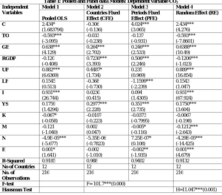
Tables 1-4 display the results of CO2 and methane gas emissions from the pooled OLS, fixed effects and random effect model. The first column of table 1 and 3 list the explanatory variables followed by several statistics. The diagnostic statistics include the R2, Hausman test and F test statistics. The number of countries in the panel, and the total number of observations both across country and over time also written in the first column. The columns in tables 1-4 present the results of separate regression models. For easy identification, the regression equations are named in columns. Column 2 to 5 of table 1 & 3 and column second, forth & sixth of table 2 & 4, the study present the results of pooled OLS, country fixed effect, period fixed effect and random effect models for CO2 and methane gas emissions respectively.

The results indicate that in model 1, coefficient of trade openness and implementation of environmental regulation has negative and statistically significant impact on CO2 emissions. This result implies that increase in trade openness and improvement in environmental regulation would reduce CO2 emissions. Coefficient of government effectiveness, urbanization, investment & trade openness generated by government efficiency have positive and significant effect on CO2 emissions. This result provide evidence that if government policies are ineffective i.e. corruption level is high, urbanization creates employment in industries and people invest in industries then consequently level of CO2 emissions would be high.

To choose FEM or REM the Hausman test should be used which has an asymptotic chi-square distribution and tests the hypothesis that FEM and REM estimators differ substantially against the null hypothesis FEM and REM estimators do not differ substantially.

The F-test has normal distribution N (0, 1) and tests the null hypothesis of insignificance as a whole of the estimated parameters, against the alternative hypothesis of significance as a whole of the estimated parameters. ***, **, and *denote significance at 1, 5 and 10 % level of significance, respectively. The figure in parentheses represents the t-statistic.

Source: Author’s calculation

Model 2 reports that the coefficients of government effectiveness, real GDP per capita, urban population, years of schooling and dummies for countries in column 2 of table 2: China, India and Indonesia have positive and statistically significant and dummies of countries Bangladesh, Malaysia, Sri Lanka, Philippines, Singapore & Honk Kong have negative and statistically significant effect on CO2 emissions. This result indicates that if government policies are ineffective, consequently CO2 emission would increase. The rapid urbanization creates congestion and employment in industries in urban areas which increase pollution. The increase level of education increases income also real GDP per capita raises demands for luxurious goods, such as automobiles, air conditioners and other electrical appliances (pollution intensive goods) therefore CO2 gas emissions would be increased.

Table 1: Pooled and Panel data Models: Dependent variable CO2

Independent Variables

Model 1 Model 2 Model 3 Model 4

Pooled OLS

Countries Fixed Effect (CFE)

Periods Fixed Effect (PFE)

Random Effect (RE)

C 2.434* (1.683794) -0.306 (-0.136) 4.024*** (3.065) 2.434*** (4.276) TO -0.593*** (-3.095) -0.033 (-0.238) -0.137 (-0.931) -0.593*** (-7.8601) GE 0.638*** (4.129) 0.264*** (2.702) 0.246*** (2.533) 0.6388*** (10.49) RGDP -0.120 (-0.408) 0.7230*** (3.393) 0.506*** (2.246) -0.1206*** (-1.023) UP 0.882*** (6.6369) 0.4487* (1.734) 0.235 (0.969) 0.889*** (16.854) LF 0.1545 (0.513) -0.368 (-0.730) -1.1599*** (-2.239) 0.1543 (1.047) I 0.931*** (26.744) 0.0230 (0.415) 0.094 (1.4305) 0.931*** (67.924) YS 0.1759 (1.4294) 0.2977*** (2.228) 0.351*** (2.735) 0.1750*** (3.604) K -0.067* (-0.058) -0.0107 (-0.223) -0.0373 (-0.7995) -0.0067 (-0.198) M -0.121 (-1.040) 0.002 (0.047) -0.005* (-0.116) -0.1212*** (-2.643) N -4.9E-05*** (-5.677) -5.35E-06 (-0.7823) 7.25E-07* (0.108) -4.29E-05*** (-14.425) E 0.001* (1.641) -0.002 (-1.010) -0.002** (-1.935) 0.001*** (4.679) R-Squared 0.9185 0.988 0.9402 0.9132 No of Countries 12 12 12 12 No. of Observations 216 216 216 216 F-test F= 101.7***(0.000) Hausman Test H=11.047***(0.001)

The results of model 3 indicate that coefficient of government effectiveness, real GDP per capita, years of schooling, implementation of environmental regulation and all period dummies (column 4 of table 2) have statistically significant and positive while trade openness, labor force participation, environmental Kuznets curve, output generated by trade openness and trade openness generated by government efficiency have negative and statistically significant effect on CO2 emissions. It means trade openness, labor force participation, and environmental Kuznets curve (higher per capita income) beneficial for environment it tends to reduce CO2 emissions. If government not efficiently implements environmental regulation policies due to corruption, also income and higher education level tends to increase CO2 emissions.

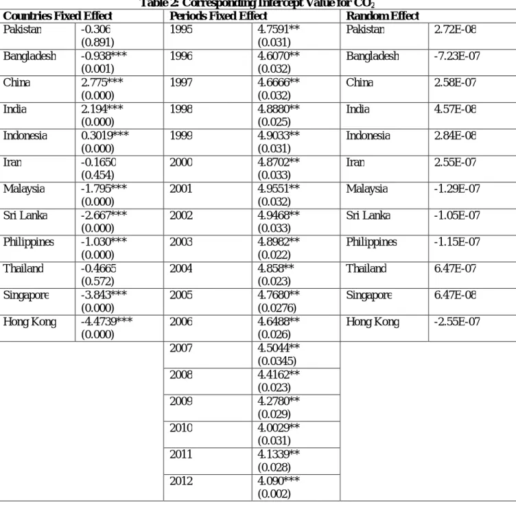
The results of random effect model for CO2 are reported in column 5 of table 1. The results of model 4 interprets that the coefficients of trade openness, government effectiveness, urbanization, investment, years of schooling, output generated by trade openness, implementation of environmental regulation and trade openness generated by government efficiency have positive and significant effect on CO2 emissions. Although trade openness, output generated by trade openness and implementation of environmental regulation have negative impact on CO2 gas emissions. This result suggests that trade openness, government effectiveness for implementation of environmental regulation and output produced by trade are beneficial for environment. Conversely urbanization, investment and years of schooling tend to increase CO2 emissions. Years of schooling increases income and demand for goods which increase industrial production, investment in industries increases pollution through production and hiring of work force, urbanization increases employment in industries which raises pollution. These results support the strength of the results from the random effects model which is the preferred model. To measure the random deviation (error component) of individual intercept from mean value of all cross-sectional intercept which is is reported in table 2, column 6. The mean value of the random error component γ is the common intercept value of 2.45. The cross-section’s random value for Pakistan is 2.72E-08 tells how much the random error component of Pakistan differs from the common intercept value. Similarly Cross-section random value of Bangladesh = -7.23E-07, China = 2.58E-07, India = 4.57E-08, Indonesia = 2.84E-08, Iran = 2.55E-07, Malaysia = -1.29E-07, Sri Lanka = -1.05E-07, Philippines = -1.15E-07, Thailand = 07, Singapore = 6.47E-08 and Hong Kong = -2.55E-07 differs from the common intercept value as given in the table 2.

Table 2: Corresponding Intercept Value for CO2

Countries Fixed Effect Periods Fixed Effect Random Effect Pakistan -0.306 (0.891) 1995 4.7591** (0.031) Pakistan 2.72E-08 Bangladesh -0.938*** (0.001) 1996 4.6070** (0.032) Bangladesh -7.23E-07 China 2.775*** (0.000) 1997 4.6666** (0.032) China 2.58E-07 India 2.194*** (0.000) 1998 4.8880** (0.025) India 4.57E-08 Indonesia 0.3019*** (0.000) 1999 4.9033** (0.031) Indonesia 2.84E-08 Iran -0.1650 (0.454) 2000 4.8702** (0.033) Iran 2.55E-07 Malaysia -1.795*** (0.000) 2001 4.9551** (0.032) Malaysia -1.29E-07 Sri Lanka -2.667*** (0.000) 2002 4.9468** (0.033)

Sri Lanka -1.05E-07 Philippines -1.030*** (0.000) 2003 4.8982** (0.022) Philippines -1.15E-07 Thailand -0.4665 (0.572) 2004 4.858** (0.023) Thailand 6.47E-07 Singapore -3.843*** (0.000) 2005 4.7680** (0.0276) Singapore 6.47E-08 Hong Kong -4.4739*** (0.000) 2006 4.6488** (0.026)

Hong Kong -2.55E-07

2007 4.5044** (0.0345) 2008 4.4162** (0.023) 2009 4.2780** (0.029) 2010 4.0029** (0.031) 2011 4.1339** (0.028) 2012 4.090*** (0.002)

***, **, and *denote significance at 1, 5 and 10 % level of significance, respectively. The figure in parentheses represents the p-values.

To choose FEM or REM the Hausman test should be used which has an asymptotic chi-square distribution and tests the hypothesis that FEM and REM estimators differ substantially against the null hypothesis FEM and REM estimators do not differ substantially. The F-test has normal distribution N (0, 1) and tests the null hypothesis of insignificance as a whole of the estimated parameters, against the alternative hypothesis of significance as a whole of the estimated parameters.

***, **, and *denote significance at 1, 5 and 10 % level of significance, respectively. The figure in parentheses represents the t-statistic.

Source: Author’s calculation

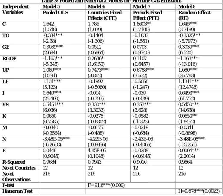
For model 5 the study reports the results from pooled regression for methane gas emissions. The regression coefficients of trade openness, real GDP per capita and implementation of environmental regulation have negative and statistically significant effect but government effectiveness, urbanization, labor force participation, investment and years of schooling have positive and statistically significant effect on methane gas emissions. So if trade is more open, increased income generates awareness and effective environmental regulation reduces pollution. In model 6, 7 this study analyzed fixed effect model for methane gas emissions. In this way the results of model 6 reported that the coefficient of government effectiveness, trade openness, labor force participation, investment, environmental Kuznets curve, output generated by trade openness, implementation of environmental regulation and trade openness generated by government efficiency have statistically insignificant effect on methane gas emissions.

Table 3: Pooled and Panel data Models for Methane Gas Emissions Independent

Variables

Model 5 Model 6 Model 7 Model 8

Pooled OLS Countries Fixed Effects (CFE) Periods Fixed Effect (PFE) Random Effect (RE) C 1.642 (1.548) 1.786 (1.039) 1.8603** (1.7100) 1.645*** (3.7199) TO -0.334*** (-2.38) -0.1404 (-1.306) -0.1833 (-1.551) -0.3325*** (-5.7973) GE 0.3039*** (2.684) 0.0512 (0.6864) 0.0703 (0.9740) 0.3039*** (6.520) RGDP -1.163*** (-5.345) 0.2636* (1.6150) 0.1107 (0.6457) -1.163*** (-13.016) UP 1.089*** (10.91) 0.7473*** (3.862) 0.6788*** (3.532) 1.080*** (26.783) LF 1.131*** (5.123) -0.1992 (-0.5060) -0.5058 (-1.247) 1.1311*** (12.4748) I 0.649*** (25.400) -0.014 (-0.393) -0.039 (-0.489) 0.6493*** (61.752) YS 0.5451*** (6.036) 0.330*** (3.3032) 0.353*** (3.628) 0.5450*** (14.638) K 0.0650 (0.7585) -0.0376 (-0.8802) -0.0582 (-1.323) 0.0650** (1.8452) M -0.0340 (-0.3564) -0.0175 (-0.488) -0.0219 (-0.684) -0.0341 (-0.8698) N -3.48E-05*** (-6.2618) -4.22E-06 (-0.8056) -2.43E-06 (-0.4066) -3.48E-05*** (-15.251) E 0.0448 (0.9045) 4.85E-05 (0.1048) -0.0289 (-0.6145) 0.0004*** (2.2014) R-Squared 0.9684 0.9943 0.9010 0.9664 No of Countries 12 12 12 12 No of Observations 216 216 216 216 F-test F= 91.6***(0.000) Hausman Test H=9.678***(0.0023)

The coefficients of real GDP per capita, urbanization, years of schooling and countries dummies (column 2 of table 4) for Bangladesh, China, India, Indonesia, Iran, Malaysia, Philippines and Thailand have positive and significant effect on methane gas emissions whereas Sri Lanka, Singapore and Honk Kong have negative and statistically significant effect on methane gas emissions. It means GDP, urbanization and years of schooling create more income so people spend more on luxurious goods, which increase methane gas emission.

Countries dummies for all time periods of model 7 (column 4 of table 4) shows significant effect on methane gas emissions but time dummies 1996, 1997, 2009 and 2010 have negative signs. In model 7 coefficient of urbanization and years of schooling have statistically significant and positive while all remaining variables have insignificant effect on methane gas emissions. It concludes that if urbanization creates jobs in industries and no. of years of schooling or education make more demand of luxurious items i.e. cars so methane gas emission also increases.

Model 8 comprises results of random effect model in which the period effect is assumed fixed. Furthermore random effect model results are more appropriate than fixed effect results. In this way results reported that regression coefficient of trade openness, Govt. effectiveness, real GDP per capita, urban population, labor force participation, investment, years of schooling, environment Kuznets curve, output generated by trade openness, implementation of environmental regulation and trade openness generated by Govt. efficiency have significant effect. Trade openness, real GDP per capita and implementation of environmental regulation have negative impact on methane gas emissions. This result implies that trade openness reduces methane gas emissions and Govt. policies are effective so people pay more tax out of their income so environment quality improves.

The mean value of the random error component γ (column 6 of table 4) is the common intercept value of 1.65. The cross-section’s random value for Pakistan is 2.50E-08 tells how much the random error component of Pakistan differs from the common intercept value. Similarly Cross-section random value of Bangladesh=-4.85E-08, China = 3.16E-Bangladesh=-4.85E-08, India = -1.24E-Bangladesh=-4.85E-08, Indonesia = -3.15E-Bangladesh=-4.85E-08, Iran = 1.47E-Bangladesh=-4.85E-08, Malaysia = 2.11E-Bangladesh=-4.85E-08, Sri Lanka = 1.63E08, Philippines = 1.20E08, Thailand = 5.34E08, Singapore = 2.18E08 and Hong Kong = -1.53E-08 differs from the common intercept value as given in the table 4.

***, **, and *denote significance at 1, 5 and 10 % level of significance, respectively. The figure in parentheses represents the p-values.

Source: Author’s calculation

7. Conclusions and Policy Implications

There has been a long debate among policy makers and economists at the national and international levels about whether trade openness and public sector corruption have impact on environmental degradation. This study conducted an empirical analysis in the framework for panel of 12 Asian countries by employing data from 1995 to 2012. This study employed fixed and random effects model for the analysis. This study also examined pooled OLS regression model to show that if country-specific features, such as law and order situations and tax structures are omitted then the pooled OLS procedure yields biased and inconsistent results especially when the omitted country and time specific variables are correlated with the explanatory variables which might affect environmental regulation. This paper tried to minimize the country and time specific heterogeneity by imposing dummies, such as, in case of fixed effect model the study used time and country specific dummies.

Table 4: Corresponding Intercept Value for Methane gas Countries Fixed Effect Periods Fixed Effect Random Effect Pakistan 1.7861** (0.0229) 1995 1.8683** (0.064) Pakistan 2.50E-08 Bangladesh 1.8428*** (0.0026) 1996 1.8042** (0.049) Bangladesh -4.85E-08 China 4.0087*** (0.000) 1997 1.7735** (0.048) China 3.16E-08 India 3.488*** (0.00) 1998 1.9876** (0.046) India -1.24E-08 Indonesia 2.088** (0.013) 1999 1.9863** (0.03) Indonesia -3.15E-08 Iran 1.0356*** (0.000) 2000 2.0537** (0.048) Iran 1.47E-08 Malaysia 0.1778*** (0.000) 2001 1.9853** (0.06) Malaysia 2.11E-08 Sri Lanka -0.0514*** (0.000) 2002 2.055** (0.045)

Sri Lanka -1.63E-08 Philippines 1.0422*** (0.000) 2003 2.0336** (0.033) Philippines 1.20E-10 Thailand 1.4108* (0.098) 2004 2.0463** (0.0417) Thailand 5.34E-08 Singapore -3.4098*** (0.000) 2005 2.0848** (0.0382) Singapore -2.18E-08 Hong Kong -3.2234*** (0.000) 2006 2.0663** (0.037)

Hong Kong -1.53E-08

2007 1.954** (0.040) 2008 1.923** (0.040) 2009 1.8093** (0.043) 2010 1.855** (0.040) 2011 1.8898** (0.036) 2012 1.8604* (0.088)

Although the random effect framework is the preferred model, but this study also presents the results from the fixed effects model for comparison purpose. That’s why study might have got more robust results, and an extended study in this area should incorporate these issues.

Further results of the random effect model concludes that there is negative and significant effect of among trade openness, government effectiveness on both CO2 and methane gas emissions. The study also suggests that trade openness generated by government efficiency entails that public sector corruption influence trade openness by their beneficial trade policies, government may import pollution abatement devices according to green policies then both gas emissions will reduce. Moreover output generated by trade openness is also have negative impact on both gas emissions it means trade openness is good for environmental health. Finally, implementation of environmental regulation depends upon on the level of corruption. If government policies are effective then people pay for environment regulations. In light of above results, policy recommendations are such that government should adopt green policies for pollution abatement also government must needs to strengthen its monitoring capability against pollution and regulate abatement technologies or devices in the light of their strategy. Side by side government should also provide proper guidance for pollution abatement by different research programs. For openness of trade, government should create trade zones, corridors and boundaries then it will enhance environmental health and stability. The world trade openness has also brought to the fore the importance of regulation of government policies towards openness as results has already warned that government effectiveness is volatile and is expected to become more tense thus the strategy needs to identify aspects of government corruption that are hurting the countries economy and reverse such strategies by adopting a more pragmatic approach.

Acknowledgements

Authors would like to acknowledge, with thanks to grateful to Mr. Sabihuddin Butt and Mr. Akhter Abdul Hai, Associate Professors at Applied Economics Research Centre (AERC), University of Karachi, for their valuable comments on plan of paper.

References

Adsera, A., & Boix, C. (2002). Trade, democracy, and the size of the public sector: The political underpinnings of openness. International Organization, 56(2), 229-262.

Andonova, L. Edward D. Mansfield and Helen V. Milner (2005) “International Trade and Environmental Policy in the Postcommunist World” hosted at http://online.sagepub.com.

A. Strutt and K. Anderson (2000), Will Trade Liberalization Harm the Environment? The Case of Indonesia to 2020 Environmental and Resource Economics 17: 203–232, 2000.

Antweiler, W., Copeland, B. and Taylor, S. (2000) “Is Free Trade Good for the Environment?” Technical Appendix. University of British Columbia.

Antweiler, W., Copeland, B. and Taylor, S. (2001) “Is Free Trade Good for the Environment?” American Economic Review, 91 (4), 877-908.

A.L. Hillman, H.W. Ursprung (1994), Greens, Supergreens and international trade policy: environmental concerns and protectionism, in: C. Carraro (Ed.), The International Dimension of Environmental Policy, Dordrecht, Kluwer.

B.R. Copeland, Tariffs and quotas: retaliation and negotiation with two instruments of protection, Journal of internet Economy. 26 (1989) 179–188.

B.R. Copeland (1994), International trade and the environment: policy reform in a polluted small open economy, Journal of Environmental Economics and Management 26 44–65.

B.R. Copeland, S.M. Taylor (1995), Trade and transboundary pollution, American Economic. Review. 85 716– 737.

Copeland, Brian R. and M. Scott Taylor (2004), Trade, Growth, and the Environment, Journal of Economic Literature 42(1), pp. 7-71.

Damania, R., P. G. Fredriksson, and J. A. List. (2003), Trade liberalization, corruption, and environmental policy formulation: theory and evidence. Journal of EnvironmentalEconomicsandManagement46(3):490-512. D. Coates (1996), Jobs versus wilderness areas: the role of campaign contributions, in: R.D. Congleton (Ed.), The

Frankel, J. and Rose, A. (2002) “Is Trade Good or Bad for the Environment? Sorting out the Causality” NBER Working Paper No. 9021. NBER Research Associates.

Frankel, Jeffrey A. and Andrew K. Rose (2005), “Is Trade Good or Bad for the Environment? Sorting Out the Causality, Review of Economics and Statistics, 87(1), pp. 85-91.

Frankel, Jeffrey A. and David Romer (1999), “Does Trade Cause Growth?, American Economic Review, 89(3), pp. 379-399.

Garrett, G. (1998). Partisan politics in the global economy. New York: Cambridge University Press. G.M. Grossman, E. Helpman, Protection for sale, Amer. Econom. Rev. 84 (1994) 833–850.

G. Schulze, H. Ursprung, The political economy of international trade and the environment, in: G. Schulze, H. Ursprung (Eds.), International Environmental Economics: A Survey of the Issues, Oxford University Press, Oxford, 2001.

Hausman, J. A. and Taylor, W. E. (1981). Panel Data and Unobservable Individual Effects. Econometrica, 49(6), 1377-1398.

Hsiao, C. (2003). Analysis of Panel Data. 2nd ed. United Kindom: Cambridge University Press, 1-7.

Hsiao, C. (2005). Why Panel Data? Department of Economics Nanyang Technological University, Singapore and University of Southern California Los Angeles, CA 90089-0253.

Kaufman, R. R., & Segura-Ubiergo, A. (2001). Globalization, domestic politics, and social spending in Latin America: A time-series cross-section analysis, 1973-97. World Politics, 53(4), 553-587.

Leite, C. and Weidmann, J. (1999) “Does Mother Nature Corrupt? Natural Resources, Corruption, and Economic Growth.” International Monetary Fund Working Paper. 99/85.

Lopez, R., and S. Mitra. 2000. Corruption, pollution, and the Kuznets environment curve. Journal of Environmental Economics and Management 40(2):137-150.

Managi, S. (2004), “Trade liberalization and the environment: carbon dioxide for 1960-1999”, Economics Bulletin, 17(1), pp. 1-5.

Mendez, F. and Sepulveda, F. (2006) “Corruption, Growth and Political Regimes: Cross Country Evidence.” European Journal of Political Economy. Vol. 22: 82-98.

Morris, Stephen D. (1991), “Corruption and Politics in Contemporary Mexico”. Tuscaloosa: University of Alabama Press.

Morse, S. 2004. Indices and indicators in development. An unhealthy obsession with numbers? Earthscan, London,UK.

M.P. Leidy, B.M. Hoekman, Cleaning Up while cleaning up? Pollution abatement, interest groups and contingent trade policies, Public Choice 78 (1994) 241–258.

R. Damania (2001), When the weak win: the role of investment in environmental lobbying, Journal of Environmental Economics and Management 42 1–22.

Poirson, H. (1998) “Economic Security, Private Investment, and Growth in Developing Countries. International Monetary Fund Working Paper, 98/4.

P.G. Fredriksson (1999), The political economy of trade liberalization and environmental policy, Southern Econom. J. 65 513–525.

P.G. Fredriksson, J. Svensson (2002), Political instability, corruption and policy formation: the case of environmental policy, Journal of Public Economics, forthcoming.

Rudra, N. (2002). Globalization and the decline of the welfare state in less-developed countries. International Organization, 56(2), 411-445.

R. Lo´ pez, S. Mitra, Corruption, pollution and the Kuznets environment curve, Journal of Environmental Economics and Management 40 (2000) 137–150.

P. Mauro, Corruption and growth, Quarterly Journal of Economics. 110 (1995) 681–712.

Shunsuke Managi (2004), Trade Liberalization and the Environment: Carbon Dioxide for 1960−1999

http://www.economicsbulletin.com/2004/volume17/pdf.

Shliefer, Andrei. (2000) "Comment on Local Corruption and Global Capital Flows." Brookings Paper on Economic Activity, Vol. 2000, No. 2: 303-354

Stepehen Morse (2007), Is Corruption Bad for Environmental Sustainability? A Cross-National Analysis. S. Coate, S. Morris, Policy Persistence, Amer. Econom. Rev. 89 (1999) 1327–1336.

Wibbels, E. (2006). Dependency revisited: International markets, business cycles, and social spending in the developing world. International Organization, 60(2), 433-468.

W. Antweiler, B.R. Copeland, M.S. Taylor, Is free trade good for the environment? American Economic Review 91 (2001) 877–908.