Analysing the effects of solution space connectivity with an effective metaheuristic for the course timetabling problem

Analysing the Effects of Solution Space Connectivity with an

Effective Metaheuristic for the Course Timetabling Problem

R. Lewis and J. Thompson

School of Mathematics, Cardiff University, CF24 4AG, Wales.

Email:

lewisR9|[email protected]

August 7, 2014

Abstract

This paper provides a mathematical treatment of the NP-hard post enrolment-based course timetabling problem and presents a powerful two-stage metaheuristic-based algorithm to approximately solve it. We focus particularly on the issue of solution space connectivity and demonstrate that when this is increased via specialised neighbourhood operators, the quality of solutions achieved is generally enhanced. Across a well-known suite of benchmark problem instances, our proposed algorithm is shown to produce results that are superior to all other methods appearing in the literature; however, we also make note of those instances where our algorithm struggles in comparison to others and offer evidence as to why.

Keywords:University timetabling; metaheuristics; solution space connectivity.

1

Introduction

Timetables are organisational structures that can be found in many areas of human activity including sports [26], en-tertainment [22], transport [15], industry [9], and education [29]. In the context of higher education institutions, a timetable can be thought of as an assignment of events (such as lectures, tutorials, or exams) to a finite number of rooms and timeslots in accordance with a set of constraints, some of which will be mandatory, and others that may be optional [21]. According to McCollum et al. [37], the problem of constructing such timetables can be divided into two categories: exam timetabling problems and course timetabling problems. It is also suggested that course timetabling problems can be further divided into two sub-categories: “post enrolment-based course timetabling”, where the con-straints of the problem are specified by student enrolment data, and “curriculum-based course timetabling”, where constraints are based on curricula specified by the university. M¨uller and Rudova [39] have also shown that these sub-categories are closely related, demonstrating how instances of the latter can be transformed into those of the former in many cases.

The field of university timetabling has seen many solution approaches proposed over the past few decades, in-cluding methods based on constructive heuristics, mathematical programming, branch and bound, and metaheuristics (see [16, 17, 29, 43] for surveys of these). A near universal constraint in problems considered in the literature is the “event-conflict” constraint, which specifies that certain pairs of events cannot be assigned to the same timeslot (e.g. there may be some students who need to attend both events). The presence of this constraint allows parallels to be drawn between timetabling and the well-known NP-hard problem of graph colouring, and it is certainly the case that heuristics derived from graph colouring are often used in timetabling algorithms [12, 18, 44].1 _{Beyond this constraint}

however, timetabling problem formulations have also tended to vary quite widely in the literature because each insti-tution usually has their own specific needs and protocols (hence constraints) that need adhering to. While making the problem area very rich, one noted drawback has been the lack of opportunity for accurate comparison of algorithms over the years [29].

In the past decade, this situation has been mitigated to a certain extent due to the organisation of a series of timetabling competitions and the release of publicly available problem instances [4, 2, 7]. In 2007, for example, the Second International Timetabling Competition (ITC2007) was organised by a group of timetabling researchers from different European Universities, which considered the three types of timetabling problems mentioned above: exam timetabling, post enrolment-based course timetabling, and curriculum-based timetabling. The competition operated by releasing problem instances into the public domain, with entrants then designing algorithms to try and solve these.

1_{Timetabling problems can be transformed into graph colouring problems by considering the events as the vertices, the timeslots as the colours,}

Entrants’ algorithms were then compared under strict time limits according to specific evaluation criteria. Further details can be found in [37] and on the competition website [2].

In this paper we give a mathematical description of the post enrolment-based course timetabling problem used for ITC2007. This particular formulation models the real-world situation where students are given a choice of lectures that they wish to attend, with the timetable then being constructed according to these choices. We present a two-stage algorithm for this problem, focussing particularly on issues surrounding solution space connectivity. We show that when this is increased via specialised neighbourhood operators combined with sensible design decisions, state of the art performance across a range of problem instances can be achieved. In Section 3, we present a review of the most noteworthy and/or recent high-performance algorithms for this problem, before going on to describe our method and its operators in Sections 4 and 5. The final results of our algorithm are given in Section 6, with a discussion and conclusions then being presented in Section 7.

2

Problem Description and Preprocessing

As mentioned, the post enrolment-based course timetabling problem was introduced for use in the Second International Timetabling Competition, run in 2007 [2, 32]. The problem involves seven “hard” constraints (described below) whose satisfaction is mandatory, and three “soft” constraints, whose satisfaction is desirable, but not essential. The problem involves assigning a set of events to 45 timeslots (5 days, with 9 timeslots per day) according to these constraints.

The hard constraints for the problem are as follows. First, for each event there is a set of students who are enrolled to attend; thus events should be assigned to timeslots such that no student is required to attend more than one event in any one timeslot. Next, each event also requires a set of room features (e.g. a certain number of seats, specialist teaching equipment, etc.), which will only be provided by certain rooms; thus each event needs to be assigned to a suitable room that exhibits the room features that it requires. The double booking of rooms is also disallowed. Hard constraints are also imposed stating that some events cannot be taught in certain timeslots. Finally, precedence constraints – stating that some events need to be scheduled before or after others – are also stipulated.

More formally, a problem instance comprises a set of eventse={e1, . . . , en}, a set of timeslotst={t1, . . . , t|t|}

(where|t|= 45), a set of studentss={s1, . . . , sm}, a set of roomsr ={r1, . . . , r|r|}, and a set of room features

f ={f1, . . . , f|f|}. Each roomri∈ris also allocated a capacityc(ri)reflecting the number of seats it contains. The relationships between these sets are defined by five matrices:

• AnattendsmatrixP(1)_m×n, whereP_i,j(1) = 1if studentsiis due to attend eventej;0otherwise.

• Aroom featuresmatrixP(2)_|r|×|f|, whereP_i,j(2)= 1if roomrihas featurefj;0otherwise.

• Anevent featuresmatrixP(3)_n×|f|, whereP_i,j(3)= 1if eventeirequires featurefj;0otherwise.

• Anevent availabilitymatrixP(4)_n×|t|, whereP_i,j(4)= 1if eventeican be assigned to timeslottj;0otherwise.

• AprecedencematrixP(5)_n×n, whereP_i,j(5) = 1if eventeishould be scheduled to an earlier timeslot than eventej;

P_i,j(5)=−1if eventeishould be scheduled to a later timeslot than eventej; and0otherwise.

For the precedence matrix above, two conditions are necessary for the relationships to be consistent: (a)P_i,j(5) = 1⇔P_j,i(5) =−1, and (b)P_i,j(5)= 0⇔P_j,i(5)= 0. We can also observe the transitivity of this relationship:

∃ei, ej, ek∈e|

P_i,j(5)= 1∧P_j,k(5) = 1⇒P_i,k(5)= 1 (1)

As noted by Lewis [30], in some of the competition problem instances this transitivity is not fully expressed; however, observing it enables further1’s and−1’s to be added toP(5)_{during preprocessing, allowing the relationships to be}

more explicitly stated.

Given the above five matrices, in our approach two further matrices are calculated, which allow fast detection of hard constraint violations during execution of the algorithm [28, 14].

• Aroom suitabilitymatrixRn×|r|, where:

Ri,j= ( 1 if Pm k=1P (1) k,i ≤c(rj) ∧@fk ∈f| P_i,k(3)= 1∧P_j,k(2)= 0 0 otherwise. (2)

• AconflictsmatrixCn×n, where: Ci,j=                    1 if ∃sk ∈s| P_k,i(1)= 1∧P_k,j(1)= 1 ∨ ∃r_k ∈r|(Ri,k= 1∧Rj,k= 1) ∧P|r| k=1Ri,k = 1 ∧P|r| k=1Rj,k= 1 ∨P_i,j(5)6= 0 ∨@tk ∈t| P_i,k(4) = 1∧P_j,k(4)= 1 0 otherwise. (3)

The matrixRspecifies the rooms that are suitable for each event (i.e. rooms that are large enough for all attending students and that have all the required features). C, meanwhile, is a symmetrical matrix (Ci,j =Cj,i) that specifies pairs of events that should not be assigned to the same timeslot (i.e. those that conflict). According to (3) this will be the case if two eventseiandejshare a common student, require the same individual room, are subject to a precedence relation, or have mutually exclusive subsets of timeslots for which they are available.

Having defined the input to this problem, a solution is represented by an ordered set of setsS = S1, . . . , S|t|

subject to the satisfaction of the following hard constraints.

|t| [ i=1 Si ⊆ e (4) Si∩Sj = ∅ (1≤i6=j≤ |t|) (5) ∀ej, ek∈Si, Cj,k = 0 (1≤i≤ |t|) (6) ∀ej ∈Si, P (4) j,i = 1 (1≤i≤ |t|) (7) ∀ej ∈Si, ek ∈Sl<i, P (5) j,k 6= 1 (1≤i≤ |t|) (8) ∀ej ∈Si, ek ∈Sl>i, P (5) j,k 6= −1 (1≤i≤ |t|) (9) Si ∈ M (1≤i≤ |t|) (10)

Constraints (4) and (5) state thatS should partition the event sete(or a subset ofe) into an ordered set of sets, labeledS1, . . . , S|t|. Each setSi∈ Scontains the events that are assigned to timeslottiin the timetable. Constraint (6) stipulates that no pair of conflicting events should be assigned to the same setSi∈ S, while Constraint (7) states that each event should be assigned to a setSi∈ Swhose corresponding timeslottiis deemed available according to matrix

P(4)_{. Constraints (8) and (9) impose the precedence requirements of the problem.}

Finally, Constraint (10) is concerned with ensuring that the events assigned to a setSi∈ Scan each be assigned to a suitable room from the room setr. To achieve this it is necessary to solve a maximum bipartite matching problem [42]. Specifically, letG= (Si, r, E)be a bipartite graph with vertex setsSi andr, and an edge set defined: E ={{ej ∈

Si, rk∈r}|Rj,k= 1}. GivenG, the setSiis a member ofMif and only if there exists a maximum bipartite matching ofGof size2|Si|, in which case the room constraints for this timeslot will have been met. In practice, such matching problems can be solved via various polynomially bounded algorithms such as the augmenting path, Hungarian, or auction algorithms [8].

In the competition’s interpretation of this problem a solutionS is consideredvalidif and only if all constraints (4)-(10) are satisfied. The quality of a valid solution is then gauged by a Distance To Feasibility (DTF) measure, calculated as the sum of the sizes of all events not contained in the solution:

DTF= X ei∈S0 m X j=1 P_i,j(1) (11) whereS0=e\(S|t|

i=1Si). If the solutionSis valid and has a DTF of zero (implyingS| t|

i=1Si=eandS0 =∅) then it is consideredfeasiblesince all of the events have been feasibly timetabled. The set of feasible solutions is thus a subset of the set of valid solutions.

2.1

Soft Constraints

As mentioned, in addition to finding a solution that obeys the hard constraints, three soft constraints are also considered in this problem.

SC1 Students should not be required to attend an event in the last timeslot of each day (i.e. timeslots 9, 18, 27, 36, or 45);

SC3 Students should not be required to attend just one event in a day.

Note that each of these soft constraints is slightly different in nature: violations of SC1 can be checked with no knowledge of the rest of the timetable; violations of SC2 can be checked when constructing a timetable; and violations of SC3 can only be checked when all events have been assigned to the timetable. The extent to which these constraints are violated is measured by a Soft Constraints Cost (SCC), which can be calculated using two further matrices:Xm×|t|,

which tells us the timeslots for which each student is attending an event, andYm×5, which specifies whether or not a

student is required to attend just one event in each of the five days.

Xi,j= ( 1 if∃ek ∈Sj|P (1) i,k = 1 0 otherwise. (12) Yi,j= ( 1 if P9 k=1Xi,9(j−1)+k = 1 0 otherwise. (13)

Using these matrices, the SCC is calculated as follows:

SCC= m X i=1 5 X j=1 (Xi,9j) + 7 X k=1 2 Y l=0 Xi,9(j−1)+k+l ! + (Yi,j) ! . (14)

Here the three terms summed in the outer parentheses of Equation 14 define the number of violations of SC1, SC2, and SC3 (respectively) for each student on each day of the timetable.

2.2

Problem Complexity

From the above descriptions, we can prove that the task of finding a feasible solution to the post enrolment-based course timetabling problem is NP-hard. LetCn×n be our symmetric conflicts matrix as defined above, filled arbitrarily. In addition, let the following conditions hold:

|r| ≥ n (15)

Ri,j = 1 ∀ei ∈e, rj ∈r (16)

P_i,j(4) = 1 ∀ei ∈e, tj∈t (17)

P_i,j(5) = 0 ∀ei, ej ∈e (18)

Here, there is an excess number of rooms which are suitable for all events (15-16), there are no event availability con-straints (17), and no precedence concon-straints (18). In this special case we are therefore only concerned with satisfying Constraints (4)-(6) while minimising the DTF, making the problem equivalent to the NP-hard partial graphk-coloring problem [10] (wherek = |t|). Thus the post enrolment-based course timetabling problem generalises an existing NP-hard problem.

From a different perspective, Cambazard et al. [14] have also shown that, in the absence of all hard constraints (6)-(10) and soft constraints SC1 and SC2, the problem of satisfying SC3 (i.e. minimising the number of occurrences of students sitting a single event in a day) is equivalent to the NP-hard set covering problem.

2.3

Evaluation

From the above descriptions, we see that a timetable’s quality is described by two values, the distance to feasibility (DTF) and the soft constraint cost (SCC). According to the competition criteria, when comparing solutions the one with the lowest DTF is deemed the best timetable, reflecting the increased importance of the hard constraints over the soft constraints. However, when two or more solutions’ DTF are equal, the winner is deemed the solution among these that has the lowest SCC.

Currently there are 24 problem instances available for this problem, all of which are known to feature at least one perfect solution (that is, a solution with DTF = 0 and SCC = 0). For comparative purposes, a benchmark timing program is also available [2] which allocates a strict time limit for each machine that it is executed on (based on its hardware and operating system). This allows entrants to use approximately the same amount of computational effort when testing their implementations, allowing more accurate comparisons.

3

Previous Approaches for this Problem

The post enrolment-based timetabling problem considered here is a generalisation of the problem model used in the first international timetabling competition run in 2003. The difference is that the latter problem does not fea-ture constraints (7-9) in its formulation. The first study into the original version of this problem was carried out by Rossi-Doria et al. in 2002 [42] who used it to compare five different metaheuristic algorithms, namely evolution-ary algorithms, simulated annealing, iterated local search, ant colony optimisation, and tabu search. Two interesting conclusions were derived from their work:

• “The performance of a metaheuristic with respect to satisfying hard constraints and soft constraints may be different”;

• “Our results suggest that a hybrid algorithm consisting of at least two phases, one for taking care of feasibility, the other taking care of minimising the number of soft constraint violations [without re-violating any of the hard constraints in the process], is a promising direction.” [42]

These conclusions have shown to be quite salient in the past decade, with the winning algorithms of both the 2003 competition and the post enrollment-based track of the 2007 competition using this suggested two-stage approach. The winning algorithm for the 2003 competition was due to Kostuch [28], who used graph colouring heuristics to gain feasibility, and then simulated annealing to try to satisfy the soft constraints. Similarly, the winning method in the 2007 competition was designed by Cambazard et al. [13], who used tabu search together with an intensification procedure for finding feasibility, and then also made use of simulated annealing for satisfying the soft constraints.

In the years following these competitions, a number of papers have been published that have equalled or improved upon the results of the 2007 competition. Cambazard et al. [14] themselves have shown how the results of their two stage competition entry can be improved by relaxing Constraint (10) such that a timeslotSi is considered feasible if|Si| <|r|. The rationale for this relaxation is that it will “increase the solution density of the underlying search space”, though a repair operator is then also needed to make sure that the timeslots satisfy Constraint (10) at the end of execution. Cambazard et al. have also examined constraint programming-based approaches and a large neighbourhood search (LNS) scheme, and find that their best results can be found when using simulated annealing together with the LNS operator for reinvigorating the search from time to time. Lewis [30] has also used a simulated annealing approach for satisfying the soft constraints of the problem and notes that, across the instances, there is a weak-to-moderate positive correlation between the connectivity of the search space and the proportion by which the SCC can be reduced by his algorithm.

Other successful algorithms for this problem have attempted to reduce violations of hard and soft constraints simul-taneously during optimisation. Ceschia et al. [19], for example, treat this problem as a single objective optimisation problem in which the space of validand invalidsolutions is explored. Specifically, they allow violations of Constraints (6), (8), and (9) within a solution, and use the number of students effected by such violations, together with the DTF to form an infeasibility measure. This is then multiplied by a weighting coefficientW and added to the SCC to form the objective function. Simulated annealing is then used to optimise this objective function and, surprisingly, after extensive parameter tuningW = 1is found to provide their best results. Nothegger et al. [40] have also attempted to optimise the DTF and SCC simultaneously, making use of ant colony optimisation to explore the space of valid solu-tions. Here the DTF and SCC are used to update the algorithm’s pheromone matrices so that favourable assignments of events to rooms and timeslots will occur with higher probability in later iterations of the algorithm. Nothegger et al. also show that the results of their algorithm can be improved by adding a local search-based improvement method and by parallelising the algorithm. Jat and Yang [25] have also used a weighted sum objective function in their hybrid evolutionary algorithm/tabu search approach, though their results do not appear as strong as those of the previous two papers. Similarly, van den Broek and Hurkens [47] have also used a weighted sum objective function in their deterministic algorithm based on column generation techniques.

From the above studies, we suggest that the density and connectivity of the underlying solution space is an im-portant issue in the performance of neighbourhood search algorithms with this problem. In particular, if connectivity is low then movements in the search space will be more restricted, perhaps making improvements in the objective function more difficult to achieve. From the research discussed above it is noticeable that some of the best approaches have attempted to alleviate this problem by relaxing some of the hard constraints [14, 19], and/or by allowing events to be kept out of the timetable [40]. However, such methods also require mechanisms for coping with these relaxations, such as repair operators (which may ultimately require large alterations to be made to a solution), or by introducing terms into the objective function (which will require appropriate weighting coefficients to be determined, perhaps via tuning). On the other hand, a two-stage approach of the type discussed by Rossi Doria et al. [42] will have no need for these features; however, because feasibility must be maintained when the SCC is being optimised (i.e. no relax-ations are permitted), the underlying solution space may be more sparsely connected, perhaps making good levels of optimisation more difficult to achieve. We will focus on this issue in Section 5 onwards.

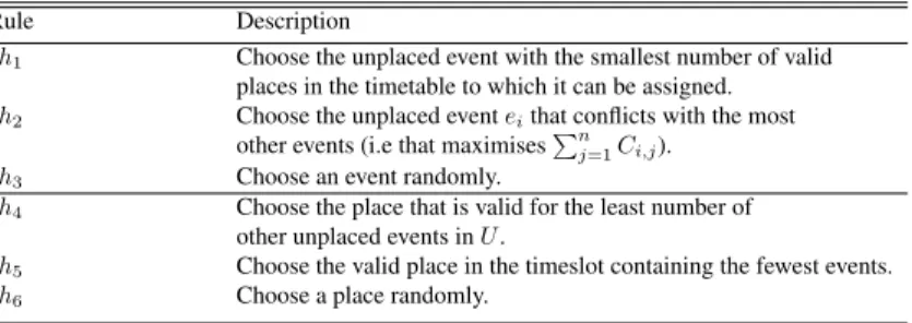
Table 1: Heuristics used for producing an initial solution in Stage 1. Here, a “valid place” is defined as a room/timeslot pair that an event can be assigned to without violating Constraints (4)-(10).

Rule Description

h1 Choose the unplaced event with the smallest number of valid

places in the timetable to which it can be assigned. h2 Choose the unplaced eventeithat conflicts with the most

other events (i.e that maximisesPn j=1Ci,j).

h3 Choose an event randomly.

h4 Choose the place that is valid for the least number of

other unplaced events inU.

h5 Choose the valid place in the timeslot containing the fewest events.

h6 Choose a place randomly.

4

Algorithm Description: Stage One

Before focussing on the task of eliminating soft constraint violations, following the two-stage approach it is first necessary to produce a valid solution that minimises the DTF measure (Equation (11)). Previous strategies for this task have typically involved inserting all events into the timetable, and then rearranging them in order to remove violations of the hard constraints [13, 14, 19, 20]. In contrast, we choose to use a method by which events are permitted to remain outside of the timetable, meaning that spaces within the timetable are not “blocked” by events causing hard constraint violations. To do this, we use an adaptation of the PARTIALCOLalgorithm, which was originally designed by Bl¨ochliger and Zufferey for use with the graph colouring problem [10, 34].

To begin, an initial solution is constructed by taking events one-by-one and assigning them to timeslots such that none of the hard constraints are violated. Events that cannot be assigned without breaking a hard constraint are kept to one side and are dealt with at the end of this process. To try and maximise the number of events inserted into the timetable, a set of high performance heuristics originally proposed in [30] and based on the DSatur graph colouring algorithm [11] is used. At each step heuristic ruleh1(Table 1) is used to select an event, with ties being broken using

h2, and thenh3(if necessary). The selected event is then inserted into the timetable according to ruleh4, breaking ties

withh5and further ties withh6.

Completion of this constructive phase results in a valid solution S obeying Constraints (4)-(10). However, if

|S0| > 0 (where S0 = e\(S|t|

i=1Si)is the set of unplaced events), the PARTIALCOL algorithm will need to be

invoked. Our version of this method operates using tabu search with the simple cost function|S0|. During a run the neighbourhood operator moves events betweenS0 and timeslots inS while maintaining the validity of the solution. Given an eventei∈S0and timeslotSj ∈ S, checks are first made to see ifeican be assigned toSjwithout violating Constraints (7)-(9). If the assignment ofei breaks one of these constraints, the move is rejected; else, all eventsek inSj that conflict withei(according toC) are transferred fromSj intoS0 and an attempt is made to insert eventei intoSj, perhaps using a maximum matching algorithm. If this is not possible (i.e. Constraint (10) cannot be satisfied) then all changes are again reset; otherwise the move is considered valid. Upon performing this change, all moves involving the re-assignment of event(s)ekto timeslotSjare considered tabu forτiterations of the algorithm. We use a tabu tenure that is a random variable proportional to the current cost,τ = b0.6× |S0|+rc, whereris an integer uniformly selected from the range 0-9 inclusive. This setting has been used in previous tabu search algorithms for graph colouring [10, 24, 34, 45] and was found to also give satisfactory results here. No tuning of this parameter was performed.

As with the original PARTIALCOLalgorithm, at each iteration the entire neighbourhood of(|S0| × |t|)moves is examined, and the move that is chosen is the one that invokes the largest decrease (or failing that, the smallest increase) in cost of any valid, non-tabu move. Ties are broken randomly, and tabu moves are also permitted if they are seen to improve on the best solution found so far. From time to time, there may also be no valid non-tabu moves available from a particular solution, in which case a randomly selected event is transferred fromS intoS0, before continuing the process as described above.

4.1

Results

Table 2 contains the results of our PARTIALCOLalgorithm and compares the results to those reported by Cambazard et al. [14], who currently claim the best results for this particular sub-problem in terms of success rates and run times.2 We report the percentage of runs in which each instance has been solved (i.e. where a DTF of zero has been achieved),

2_{Our algorithm was implemented in C++, and all experiments in this paper were conducted on 3.0 GHz Windows 7 PCs with 3.87GB RAM.}

Table 2: Comparison of results of the LS-colouring method of Cambazard et al. [14], and our PARTIALCOL and Improved PARTIALCOLalgorithms (all figures taken from 100 runs per instance).

Instance # 1 2 3 4 5 6 7 8 9 10 11 12

Cambazard et al. % Solved 100 100 100 100 100 100 100 100 100 98 100 100 Avg. time (s) 11.60 37.10 0.37 0.43 3.58 4.32 1.84 1.11 51.73 170.24 0.40 0.64 PARTIALCOL % Solved 100 100 100 100 100 100 100 100 100 100 98 100 Avg. time (s) 0.25 0.79 0.02 0.04 0.05 0.07 0.02 0.01 0.71 1.80 1.88 0.04 Improved PARTIALCOL % Solved 100 100 100 100 100 100 100 100 100 100 100 100 Avg. time (s) 0.25 0.79 0.02 0.02 0.06 0.08 0.03 0.01 0.68 2.03 0.03 0.04

Instance # 13 14 15 16 17 18 19 20 21 22 23 24 Cambazard et al. % Solved 100 100 100 100 - - - -Avg. time (s) 8.86 7.97 0.80 0.55 - - - -PARTIALCOL % Solved 100 100 100 100 100 100 100 100 100 100 100 100 Avg. time (s) 0.08 0.11 0.01 0.01 0.00 0.02 0.74 0.01 0.07 3.77 1.33 0.17 Improved PARTIALCOL % Solved 100 100 100 100 100 100 100 100 100 100 100 100 Avg. time (s) 0.08 0.11 0.01 0.01 0.00 0.02 0.71 0.01 0.08 3.80 1.10 0.18

and the average time that this took (calculated only from the solved runs).3 We see that the success rates for the two approaches are similar, with all except one instance being solved in 100% of cases (instance #10 in Cambazard et al.’s case, instance #11 in ours). However, with the exception of instance #11, the time required by PARTIALCOLis considerably less, with an average reduction of 97.4% in CPU time achieved across the 15 remaining instances.

Curiously, when using our PARTIALCOLalgorithm with instance #11, most of the runs were solved very quickly. However in a small number of runs, the algorithm seemed to quickly navigate to a point in which a small number of events remained unplaced and where no further improvements could be made, suggesting the search was caught in a conspicuous valley in the cost landscape. To remedy this situation we therefore added a diversification mechanism to the method which attempts to break out of such regions. We call this our improved PARTIALCOLalgorithm and its results are also given in Table 2.

In the improved PARTIALCOLmethod, our diversification mechanism is used for making relatively large changes to the incumbent solution, allowing new regions of the search space to be explored. It is called when the best solution found so far has not been improved for a set number of iterations. The mechanism operates by first randomly selecting a percentage of events inSand transferring them to the set of unplaced eventsS0. Next, alterations are made toSby performing a random walk using neighbourhood operatorN5(described in Section 5). Finally, the tabu list is reset so

that all potential moves are deemed non-tabu, before PARTIALCOLcontinues to execute as before. For the results in Table 2, the diversification mechanism was called after 5000 non-improving iterations, and extracted 10% of all events inS. A random walk of 100 neighbourhood moves was then performed, giving a>95%chance of all timeslots being altered by the neighbourhood operator (a number of other parameters were also tried here, though few differences in performance were observed). We see that the improved PARTIALCOLmethod has achieved feasibility in all runs in the sample, with the average time reduction remaining at 97.4% compared to Cambazard et al. [14].

5

Algorithm Description: Stage Two

5.1

Cooling Scheme

In the second stage of this algorithm simulated annealing (SA) [27] is used to explore the space of valid/feasible solu-tions, attempting to minimise the number of soft constraint violations (measured by the SCC given in Equation (14)). This metaheuristic is applied in a straightforward manner: starting at an initial “temperature”T0, during execution the

temperature variable is slowly reduced according to an update ruleTi+1=αTi, whereα(0< α <1)is known as the

“cooling rate”. As with our earlier work [30], at each temperatureTi, a Markov chain is generated by performingn2

applications of the neighbourhood operator. Moves that are seen to violate a hard constraint are immediately rejected. Moves that preserve feasibility but that increase the cost of the solution are accepted with probability exp(−δ/Ti) (whereδis the change in cost), while moves that reduce or maintain the cost are always accepted. The initial tem-peratureT0is calculated automatically by performing a small sample of neighbourhood moves and using the standard

3_{For comparative purposes, the computation times stated by Cambazard et al. [14] have been altered in Table 2 to reflect the increased speed of}

our machines. Specifically, according to Cambazard et al. the competition benchmark program allocated them 324s per run. Hence, Cambazard et al.’s original run times have been reduced by 23.8%. We should note, however, that when comparing algorithms in this way, discrepancies in results and times can also occur due to differences in the hardware, operating system, programming language, and compiler options that are used. Our use of the competition benchmark program attempts to reduce discrepancies caused by the first two factors, but cannot correct for differences arising due to the latter two.

deviation of the cost over these moves [48].

Because this algorithm operates according to a time limit, our value forαis determined automatically so that the temperature is reduced as slowly as possible betweenT0and some end temperatureTend. In existing research [30, 14,

28] this has been achieved by performing a short preliminary run of SA to gauge the speed at which the algorithm operates, allowing the number of Markov chains generated during the entire runµto be estimated. The cooling rate is then fixed toα= (Tend/T0)1/µ. However, in our implementation we found this method of estimation to be inadequate

because the time taken to complete each Markov chain also seems to depend on the temperature itself, makingµ

difficult to estimate accurately.4 In our case we therefore use a different method wherebyαis modified during a run according to the length of time that each Markov chain takes to generate. Specifically, letµ∗ denote the estimated number of Markov chains that will be completed in the remainder of the run, calculated by dividing the amount of remaining run time by the length of time the most recent Markov chain (operating at temperatureTi) took to generate. On completion of theith Markov chain, a modified cooling rate can thus be calculated as:

αi+1= (Tend/Ti)1/µ

∗

(19)

The upshot is that the cooling rate will be altered slightly during a run, allowing the user-specified end temperature

Tendto be reached at the time limit. Suitable values forTend, the only parameter required for this phase, are examined in Section 6.

5.2

Neighbourhood operators

We now define a number of different neighbourhood operators that can be used in conjunction with the SA algorithm. LetN(S)be the set of candidate solutions in the neighbourhood of the incumbent solutionS. Also, letSbe the set of

all valid solutions (i.e. S ∈Sif and only if Constraints (4)-(10) are satisfied). The relationship between the solution

space and neighbourhood operator can be conveniently defined by a graphG= (S, E)with vertex setSand edge set

E={(S ∈S,S0∈S)|S0∈N(S)}. In our case, since all our neighbourhood operators are reversible,Gis defined as

a simple graph, i.e.(S,S0_{)∈E ⇔(S}0_{,S)∈E. The various neighbourhood operators are now defined.}

N1: The first neighbourhood operator is based on those used by Lewis [30] and Nothegger et al. [40]. Consider a valid

solutionSrepresented as a matrixZ|r|×|t|in which rows represent rooms and columns represent timeslots. Each

element ofZcan be blank or can be occupied by exactly one event. IfZi,j is blank, then roomriisvacant in timeslot tj. IfZi,j = ek, thenek is assigned to roomri and timeslottj. N1 operates by first randomly

selecting an elementZi1,j1containing an arbitrary eventek. A second elementZi2,j2is then randomly selected in a different timeslot (j16=j2). IfZi2,j2is blank, the operator attempts to transferekfrom timeslotj1into any vacant room in timeslotj2. IfZi2,j2 =el, then a swap is attempted in whichekis moved into any vacant room in timeslotj2, andelis moved into any vacant room in timeslotj1. If such changes are seen to violate any of the

hard constraints, they are rejected immediately, else they are kept and the new solution is evaluated according to Equation (14).

N2: This operates in the same manner asN1. However, when seeking to insert an event into a timeslot, if no vacant,

suitable room is available, a maximum matching algorithm is also executed to determine if a valid room alloca-tion of the events can be found. A similar operator was used by Cambazard et al. in their winning competialloca-tion entry [13].

N3: This is an extension ofN2. Specifically, if the proposed move inN2will result in a violation of Constraint (6),

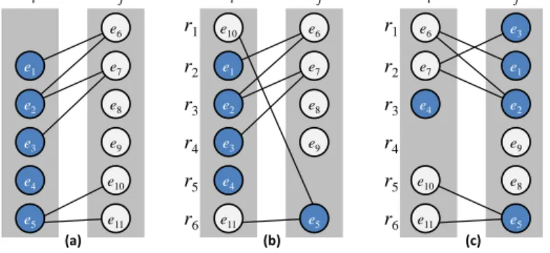
then a Kempe chain interchange is attempted [44, 20, 33]. Kempe chains are derived from the underlying graph colouring model and correspond to connected sub-graphs containing vertices (events) in two colour classes (timeslots). An example of this process is shown in Figure 1(a). Imagine in this case that we have chosen to swap the eventse5∈Siande10∈Sj. However, doing so would violate Constraint (6) because eventse5ande11

conflict but would now be assigned to the same timeslot, rendering the move invalid. In this case we therefore construct a Kempe chain frome5 which, when interchanged, guarantees the preservation of Constraint (6), as

shown in Figure 1(b). Note however that, as with the previous neighbourhood operators, a Kempe interchange might not preserve the satisfaction of the remaining hard constraints, and will need to be rejected if this is the case.

N4: This operator extendsN3by using the idea of double Kempe chains, originally proposed by L¨u and Hao [36].

In many cases, a proposed Kempe chain interchange will be rejected because it will violate Constraint (10): i.e. suitable rooms cannot be found for all of the events proposed for assignment to a timeslot. For example, in Figure 1(a) the proposed Kempe interchange involving events {e1, e2, e3, e6, e7} is guaranteed to violate

4_{In essence, this is because at lower temperatures a greater proportion of moves are rejected, with the associated cost matricesXandYhaving to}

be reset more frequently. These extra operations generally result in low-temperature Markov chains taking longer to generate than high-temperature chains.

Si Sj r₁ r2 r₃ r₄ r₅ r6 e1 e2 e3 e4 e5 e6 e7 e8 e9 e10 e11 Si Sj r₁ r2 r₃ r₄ r₅ r6 e1 e2 e3 e4 e6 e7 e8 e9 e10 e11 e5 (a) (b) r₁ r2 r₃ r₄ r₅ r6 e1 e2 e3 e4 e6 e7 e8 e9 e10 e11 e5 (c) Si Sj

Figure 1: Example moves usingN3 andN4. Here, edges exist between pairs of vertices (events)ek, elif and only if Ck,l = 1. Figure (a) shows two timeslots containing two Kempe chains,{e1, e2, e3, e6, e7} and{e5, e10, e11},

respectively; Figure (b) shows a result of interchanging the latter chain; (c) shows the result of interchanging both chains. Note that room allocations are determined via a matching algorithm and may alter during an interchange.

Constraint (10) because it will result in too many events in timeslotSj for a feasible matching to be possible. However, applying a second Kempe chain at the same time may result in feasibility being maintained, as is illustrated in Figure 1(c).

In this operator, if a proposed single Kempe chain interchange is seen to violate Constraint (10) only, then a ran-dom vertex from one of the two timeslots, but from outside this chain is ranran-domly selected, and a second Kempe chain is formed from it. If the proposed interchange of both Kempe chains does not violate any of the hard constraints, then the move can be performed and the new solution can be evaluated according to Equation (14) as before.

N5: Finally,N5defines a multi-Kempe chain interchange operator. This generalisesN4in that if a proposed double

Kempe chain interchange is seen to violate Constraint (10) only, then triple Kempe chains, quadruple Kempe chains (and so on) can also be investigated in the same manner. Note that when constructing these multiple Kempe chains, a violation of any of the constraints (7)-(9) will mean that we can reject the move immediately. However, if only Constraint (10) continues to be violated, then eventually the considered Kempe chains will contain all events in both timeslots, in which case the move will become equivalent to the swapping of the contents of the two timeslots. Trivially, in such a move Constraint (10) is guaranteed to be satisfied.

From the above descriptions it is clear that each successive neighbourhood operator is more expensive than its predecessor. However, each operator also generalises its predecessor – that is,N1(S)⊆N2(S)⊆. . .⊆N5(S),∀S ∈ S. From the perspective of the graphG = (S, E)defined above, this implies a greater connectivity of the solution

space sinceE1⊆E2 ⊆. . .⊆E5(whereEi ={(S,S0)|S0 ∈Ni(S)}fori= 1, . . . ,5). Note though, that the set of verticesSremains the same under the different operators.

Finally, it is worth mentioning that each of the above operators only ever alters the contents of two timeslots in any particular move. In practice, this means that we only need to consider the particular days and students affected by the move when re-evaluating the solution according to Equation (14). This allows considerable speed-up of the algorithm.

5.3

Dummy Rooms

An additional way by which the connectivity of the underlying solution space might be enhanced is through the use of “dummy rooms”. A dummy room is an extra room made available in all timeslots and defined as suitable for all events (i.e. it has an infinite seating capacity and possesses all available room features). Dummy rooms can be used with any of the previous neighbourhood operators, and multiple dummy rooms can also be applied if necessary. We therefore useN_i(j)to denote the use of neighbourhoodNiusingjdummy rooms (giving|r|+jrooms in total). Similarly, we can use the notationS(j)to denote the space of all solutions that obey all hard constraints, and wherejdummy rooms

are available. (For brevity, where a superscript is not used, we assume no dummy room is being used.) Dummy rooms can be viewed as a type of “placeholder” that are used to contain events not currently assigned to the “real” timetable. Transferring events in and out of dummy rooms might therefore be seen as similar to moving events in and out of the timetable.

Note that the use of dummy rooms increases the size of the setM, making Constraint (10) easier to satisfy. This leads to the situation depicted in Figure 2. Here, we observe that the presence of dummy rooms increases the number of vertices/solutions (i.e. S(j) ⊆ S(j+1), ∀j ≥ 0), with extra edges (dotted in the figure) being created between

some of the original vertices and new vertices. As depicted, this may allow previously disjoint sub-graphs to become connected.

Feasible solution Solution with one or more events assigned to a dummy room

(a) (b)

Figure 2: Graphs depicting the connectivity of a solution space with (a) no dummy rooms(S), and (b) one or more

dummy rooms (S(j>0)). 0 0.02 0.04 0.06 0.08 0.1 0.12 10 22 2 9 1 20 21 13 14 19 24 5 6 15 16 8 18 23 12 7 11 4 3 17 Feas ibi lity Rati o Instance # 1 2 3 4 100 100+1DR N1 N2 N3 N4 N5 N5(1)

Figure 3: Feasibility ratio for neighbourhood operatorsN1. . . N5and alsoN (1)

5 for all 24 problem instances.

Because they do not form part of the original problem, at the end of the optimisation process all dummy rooms will need to be removed, meaning that any events assigned to these will contribute to the DTF measure. Because this is undesirable, in our case we attempt to discourage the assignment of events to the dummy rooms during evaluation by considering all events assigned to a dummy room as unplaced. We then use the cost functionW ×DTF+SCP, whereW is a weighting coefficient that will need to be set by the user. Additionally, when employing the maximum matching algorithm we ensure that the dummy room is only used when necessary – that is, if a maximum matching can be achieved without using a dummy room, then this is the one that will be used.

5.4

Estimating Solution Space Connectivity

We have now seen various neighbourhood operators for this problem and made some observations on the connectivity of their underlying search spaces, defined byG. Unfortunately however, it will usually be very difficult to gain a complete understanding of the connectivity ofGbecause it will simply be too large to enumerate. In particular, we are unlikely to be able to confirm whetherGis connected or not, which would be useful information if we wanted to know whether the optimal solution could be reached from any other solution within the solution space.

One way we might gain an indication of G’s connectivity is to make use of what we will call the feasibility ratio. This is defined as the proportion of proposed neighbourhood moves that are seen to not violate any of the hard constraints (i.e. that maintain validity/feasibility). A lower feasibility ratio therefore suggests a lower connectivity inGbecause, on average, more potential moves will be seen to violate a hard constraint from a particular solution, meaning movements within the solution space are more restricted. A higher feasibility ratio will suggest a greater connectivity.

Figure 3 displays the feasibility ratios for neighbourhood operatorsN1. . . N5 and alsoN (1)

5 for all 24 problem

instances. These mean figures were found by performing random walks of 50,000 feasible-preserving moves with each operator from a sample of 20 feasible solutions per instance (produced via Stage 1). As expected, we see that the feasibility ratios increase for each successive neighbourhood operator, though the differences betweenN3,N4, and

N5appear to be only marginal. We also observe quite a large range across the instances, with instance #10 appearing

to exhibit the least connected solution space (with feasibility ratios ranging from just 0.0005 (N1) to 0.004 (N (1)

5 )),

and instance #17 having the highest levels of connectivity (0.04 (N1) to 0.10 (N (1)

5 )). Standard deviations from these

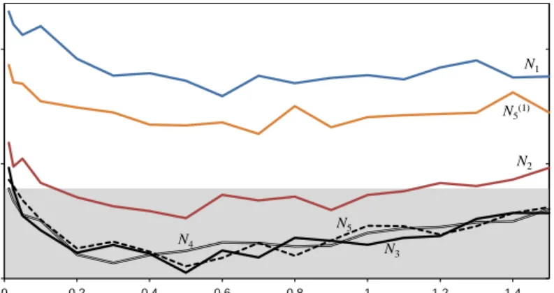
15 20 25 0 0.2 0.4 0.6 0.8 1 1.2 1.4 N1 N2 N5(1) N3 N4 N5

End Temperature: Tend

R

ank

ing

Scor

e

Figure 4: Ranking scores achieved by the different neighbourhood operators using different end temperatures. The shaded area indicates the results that would have won the competition.

6

Experimental Results

6.1

Effect of Neighbourhood Operators

In our first set of experiments we examine the ability of each neighbourhood operator to reduce the soft constraint cost within the time limit specified by the competition benchmarking program (minus the time used for Stage 1). We also consider the effects of alteringTend– the only run-time parameter required in this stage. To measure performance, we compare our results to those achieved by the five finalists of the competition using the competition’s ranking system. This involves calculating a “ranking score” for each algorithm, derived as follows.

Givenxalgorithms and a single problem instance, each algorithm is executedytimes, givingxyresults. These results are then ranked from 1 toxy, with ties receiving a rank equal to the average of the ranks they span. The mean of the ranks assigned to each algorithm is then calculated, giving the respective rank scores for thexalgorithms on this instance. This process is then repeated on all instances, and the mean of all ranking scores of each algorithm is taken as its overall ranking score. The best ranking score achievable for an algorithm is therefore(y+ 1)/2, (in which case its results are better than all other algorithms’ in all cases); the worst possible score is(x−1)y+ (y+ 1)/2. A worked example of this process can be found in [37].

A full breakdown of the results and ranking scores of the five competition finalists can be found at [2], wherex= 5

andy = 10. In our case, we added results from ten runs of our algorithm to these published results, givingx = 6,

y = 10. A summary of the resultant ranking scores achieved by our algorithm with each neighbourhood operator over a range of different settings forTend is given in Figure 4. The shaded area of the figure indicates those settings where our algorithm would have won the competition (i.e. that have achieved a lower ranking score than the other five entries).

Figure 4 shows a clear difference in the performance of neighbourhood operators N1 andN2, illustrating the

importance of the extra connectivity provided by the maximum matching algorithm. Similarly, the results ofN3,N4

andN5are better still, outperformingN1 andN2across all the values ofTendtested. However, there is very little

difference between the performance ofN3,N4andN5themselves presumably due to the fact that, for these particular

problem instances, the behaviour and therefore feasibility ratios of these operators are very similar (refer to Figure 3). Moreover, the extra expense ofN5overN3andN4appears to have minimal effect, withN5producing less than 0.5%

fewer Markov chains than N3 over the course of the run on average. Of course, such similarities will not always

be the case – they merely seem to be occurring with these particular problem instances because, in most cases, hard constraints are being broken (and the move rejected) before the inspection of more than one Kempe chain is deemed necessary.

Figure 4 also shows that the use of dummy rooms does not seem to improve results across the instances. In initial experiments we tested the use of 1 and 2 dummy rooms along with a range of different values for the weighting coefficientW ∈ {1,2,5,10,20,200,∞}.5_{Figure 4 reports the best of these: 1 dummy room withW = 2. For higher}

values ofW, results were found to be inferior because the additional solutions in the search space (shaded vertices in Figure 2) would still be evaluated by the algorithm, but nearly always rejected due to their high cost.6 _{On the other}

5_{Some of these values were chosen due to their use in existing algorithms using weighted sum functions with this problem [19, 40, 47].} 6_{We might consider the use of no dummy rooms as similar to usingW≈ ∞, in that the algorithm will not accept moves that involve moving}

an event into a dummy room (i.e. introducing infeasibility to the timetable). However the difference is that when using dummy rooms, such moves will still be evaluated by the algorithm before being rejected while, when using no dummy rooms, these unnecessary evaluations will not take place, saving significant amounts of time during the course of a run.

0 0.25 0.5 0.75 1 0 0.02 0.04 0.06 0.08 0.1 0.12 P ropo rti on Redu c ti on in Cos t Feasibility Ratio N1 N5 N₁ N₅

Figure 5: Scatter plot showing the relationship between feasibility ratio and reduction in cost for the 24 competition instances, using neighbourhood operatorsN1andN5.

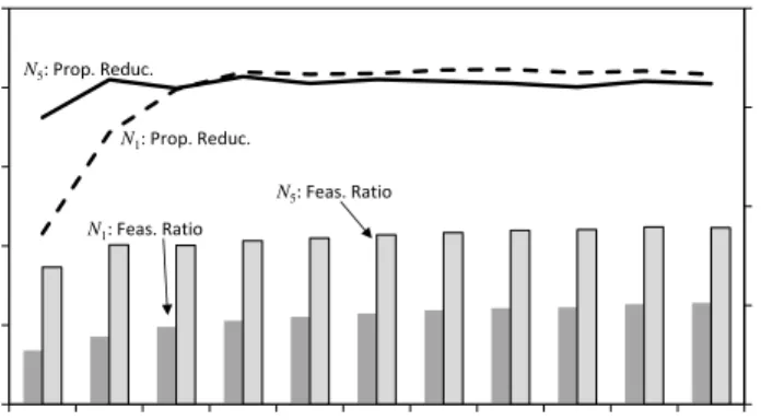
0.6 0.7 0.8 0.9 1 0.02 0.04 0.06 0.08 0.1 0.12 0 1 2 3 4 5 6 7 8 9 10 Proport ion R educ tion in C os t F eas ibilit y R at io Dummy Rooms N1: Feas. Ratio N5: Feas. Ratio N5: Prop. Reduc. N1: Prop. Reduc.

Figure 6: Effect of adding dummy rooms on (a) the feasibility ratio and (b) the proportion reduction in cost forN1

andN5, usingW = 0. (Mean of 10 runs on all 24 instances).

hand, using the settingW = 1means that the penalty of assigning an event to a dummy room will be equal to the penalty of assigning the event to the last timeslot of a day (soft constraint SC1), meaning there is little distinction between the cost of infeasibility and the cost of soft constraint violations.

As mentioned, a setting ofW = 2, which seems the best compromise of these extremes, still produces inferior results on average compared to using no dummy rooms. However, for problem instance #10 we found the opposite to be true, with significantly better results being produced when using dummy rooms. From Figure 3, we observe that #10 has the lowest feasibility ratio of all instances, and so the extra connectivity provided by the dummy rooms seems to be aiding the search in this case. On the other hand, the existence of a perfect solution here could mean that, while optimising the SCC, the search might also be being simultaneously guided towards regions of the solution space that are feasible. This matter will be examined further in Section 6.3.

Figure 5 illustrates for the 24 problem instances the relationship between the feasibility ratio and the proportion by which the SCC is reduced by the SA algorithm for two contrasting neighbourhood operators. We see that the points for

N5are shifted upwards and rightwards compared toN1illustrating the larger feasibility ratios and higher performance

of the operator. The general pattern in the figure suggests that higher feasibility ratios allow large decreases in cost during a run, while lower feasibility ratios can result in both large or small decreases, depending on the instance. Thus, while there is some relationship between the two variables, it seems likely that other factors also have an impact here, including the size and shape of the cost landscape and the amount of computation needed for each application of the evaluation function.

Finally, Figure 6 demonstrates the effect of introducing a larger number of dummy rooms into the solution. This generally increases the feasibility ratio because Constraint (10) becomes easier to satisfy; however, this increase also levels off due to hard constraints (4)-(9) remaining. As a result, there is also a levelling off in the amount that the SCC is reduced during the run. (Note that this does not imply that better overall results can be achieved when using large

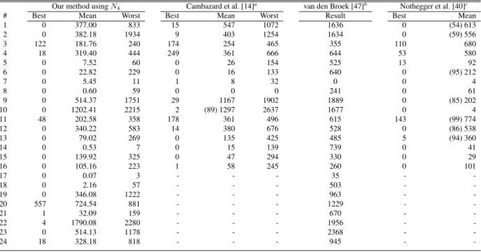
Table 3: Results from the literature, taken from samples of 100 runs. Figures indicate the SCC achieved at the cut-off point defined by the competition benchmarking program. Numbers in parentheses indicate % of runs where feasibility was found. No parentheses indicates feasibility was achieved in all runs.

Our method usingN4 Cambazard et al. [14]a van den Broek [47]b Nothegger et al. [40]c

# Best Mean Worst Best Mean Worst Result Best Mean

1 0 377.00 833 15 547 1072 1636 0 (54) 613 2 0 382.18 1934 9 403 1254 1634 0 (59) 556 3 122 181.76 240 174 254 465 355 110 680 4 18 319.40 444 249 361 666 644 53 580 5 0 7.52 60 0 26 154 525 13 92 6 0 22.82 229 0 16 133 640 0 (95) 212 7 0 5.45 11 1 8 32 0 0 4 8 0 0.60 59 0 0 0 241 0 61 9 0 514.37 1751 29 1167 1902 1889 0 (85) 202 10 0 1202.41 2215 2 (89) 1297 2637 1677 0 4 11 48 202.58 358 178 361 496 615 143 (99) 774 12 0 340.22 583 14 380 676 528 0 (86) 538 13 0 79.02 269 0 135 425 485 5 (94) 360 14 0 0.53 7 0 15 139 739 0 41 15 0 139.92 325 0 47 294 330 0 29 16 0 105.16 223 1 58 245 260 0 101 17 0 0.07 3 - - - 35 - -18 0 2.16 57 - - - 503 - -19 0 346.08 1222 - - - 963 - -20 557 724.54 881 - - - 1229 - -21 1 32.09 159 - - - 670 - -22 4 1790.08 2280 - - - 1956 - -23 0 514.13 1178 - - - 2368 - -24 18 328.18 818 - - - 945 -

-a_{Results of Cambazard et al’s SA-colouring method, [14] pp. 122.}

b_{Deterministic IP-based heuristic, thus only one result reported per instance, [47] pp. 451.} c_{Serial ACO algorithm, [40] pp. 334.}

numbers of dummy rooms, since a weighting ofW = 0has been used for this example.)

6.2

Comparison to Published Results

In our next set of experiments, we compare the performance of our algorithm to the best results reported for this problem since 2007. Table 3 gives a breakdown of the results achieved by our method usingTend =0.5 compared

to the approaches of van den Broek and Hurkins [47], Cambazard et al. [14], and Nothegger et al. [40]. The latter two papers only list results for the first 16 instances. In this table, all statistics are calculated from 100 runs on each instance (with the exception of van den Broek and Hurkins whose algorithm is deterministic), and all results have been achieved strictly within the time limits specified by the competition benchmark program. Our experiments were performed usingN3,N4, andN5, though no significant difference was observed between the three operators’ best,

mean, or worst results. Hence we only present the results of one of these,N4, here.7

Table 3 shows that, usingN4, perfect solutions have been achieved by our method in 17 of the 24 problem instances.

A comparison to the 16 results reported by Cambazard et al. indicates that our method’s best, mean, and worst results are also significantly better than their corresponding results. Similarly, our best, mean, and worst results are all seen to outperform the results of van den Broek and Hurkins [47]. Finally, no significant difference is observed between the best and mean results of our method compared to Nothegger et al. [40]; however, unlike our algorithm they have failed to achieve feasibility in a number of cases.

Another method reporting strong results, and for which source code is also available, is due to Ceschia et al. [19, 1]. In their paper, the authors have performed extensive parameter tuning via an automated method and have also used an iteration limit to define the stopping criteria instead of the competition benchmark program. In practice this latter point makes it difficult to compare their published results to those in Table 3 because, in our repetition of their experiments, runs of their algorithm to their stated iteration limits were found to exceed the benchmark time limit by between 24% and 165%. To gain a more indicative comparison, we therefore repeated their published experiments, and used the resultant run times of their implementation as time limits for our own algorithm.

Table 4 gives the ranking scores for the two algorithms on each instance. These are calculated from 10 runs per algorithm (i.e. x = 2,y = 10), giving ranking scores of between 5.5 and 15.5. We see that our approach has outperformed Ceschia et al.’s method in 18 of the 24 instances, with one instance (#16) tied. In three instances (#9, #19,

7_{For pairwise comparisons, Related Samples Wilcoxon Signed Rank Tests were used; for other comparisons Friedman Tests were used}

Table 4: Ranking scores achieved by our method and Ceschia et al.’s method [19] for all 24 problem instances (10 runs per instance). % Time Increase indicates the amount the time limit was extended beyond the limit imposed by the competition benchmark program, calculated as(1−time1/time2)×100, where time1gives the average time taken to

run the method of [19] on each instance, and time2gives the competition time limit on the same machine).

Instance # 1 2 3 4 5 6 7 8 9 10 11 12

% Time Increase 62 67 151 146 24 29 50 54 96 78 142 137 Our Method 9.6 7 5.75 6.2 7.5 7.8 11 8 5.5 12.6 6 7.1

Ceschia et al. [19] 11.4 14 15.25 14.8 13.5 13.2 10 13 15.5 8.4 15 13.9

Instance # 13 14 15 16 17 18 19 20 21 22 23 24

% Time Increase 27 26 59 70 112 64 132 142 39 89 165 131 Mean Our Method 8.35 8.8 11.85 10.5 10 7 5.5 8.2 8.65 14.5 5.5 11.3 8.51

Ceschia et al. [19] 12.65 12.2 9.15 10.5 11 14 15.5 12.8 12.35 6.5 15.5 9.7 12.50

Table 5: Contingency table showing the number of instances (out of 40) where each method outperforms the other. Instances are divided into those where a perfect solution is known to exist, and those where this is unknown. Values in parentheses indicate the average rank scores of the algorithms on these instances.

Known Unknown Our Method 4.5 (7.14) 21 (6.20) Ceschia et al. [19] 12.5 (6.33) 2 (5.65)

#23) these ranking scores are also at their extremes, indicating that all ten runs with our method have outperformed those of Ceschia et al.

6.3

One-Stage Versus Two-Stage Approaches

A noteworthy feature of the results given in Tables 3 and 4 is that, in contrast to the approaches of Ceschia et al. [19] and Nothegger et al. [40], our method has performed relatively poorly with a small number of problem instances, most notably #10 and #22. According to Figure 3, these instances also exhibit the lowest feasibility ratios with our operators, suggesting that freedom of movement in the search space is too restricted to allow adequate optimisation of the objective function.

On the other hand, it is also possible that the algorithms of Ceschia et al. and Nothegger et al. are being aided by the fact that perfect solutions to the 24 competition instances are known to exist – a feature that is unlikely to occur in real world problem instances. For example, as noted in Section 3, Ceschia et al.’s algorithm has produced its best results with the competition instances when optimisation is performed using an objective function in which hard and soft constraint are given equal weights. However it could be that, by moving towards solutions with low SCCs, the search could also inadvertently be moving towards feasible regions of the search space, simultaneously helping to satisfy the hard constraints along the way.

To test this hypothesis we repeated our experiments with Ceschia et al.’s method and our own using a second set of publicly available problem instances, the so-called “harder” problem instances. This set of instances has previously been used in the literature for testing algorithms’ ability to find feasibility only [19, 23, 31, 35, 38, 41, 46] and they differ to the 24 competition instances in that they do not consider Constraints (8)-(10), and only some are known to feature perfect solutions (though they do all feature a feasible solution).8 _{In our tests both algorithms were executed}

ten times on the forty largest instances from this set, of which 17 are known to feature perfect solutions. Because our algorithm was not able to able to achieve feasibility in seven of the forty instances, a maximum limit of 50% of the time run time was allocated to Stage 1, with the remainder given to Stage 2.

Table 5 summarises the results of these trials. For each problem instance a ranking score of between 5.5 and 15.5 was calculated for each algorithm, and the number of instances that each algorithm outperformed the other, together with the average ranking scores across these instances is presented. The results strongly support our hypothesis: for the 23 instances with no known perfect solution, our algorithm has outperformed Ceschia et al.’s in 21 cases (91.3%). Moreover, the average ranking score across these instances (6.2) is close to the minimum possible, indicating that this difference is stark. On the other hand, with the remaining 17 instances, Ceschia et al.’s approach has produced better results in 12.5 cases (73.5%), suggesting that the existence of perfect solutions is indeed benefitting the algorithm.

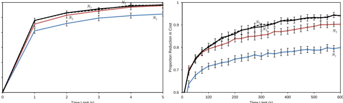
0 0.1 0.2 0.3 0.4 0.5 0.6 0 1 2 3 4 5 P rop orti on Red ucti on In Cost Time Limit (s) N1 N2 N3 N5 0.6 0.7 0.8 0.9 1 0 100 200 300 400 500 600 P rop or ti on Red uc ti on i n Cos t Time Limit (s) N1 N2 N5 N3

Figure 7: Proportion decrease in SCC using differing time limits and differing neighbourhood operators. All points are taken from an average of 10 runs on each problem instances (i.e. 240 runs). Error bars, shown forN1,N2, and

N3, represent one standard error each side of the mean.

6.4

Differing Time Limits

In our final set of experiments we look at the effects of using differing time limits with our algorithm. Until this point, most experiments have been performed according to the time limit specified by the competition benchmark program;9 however, it is pertinent to ask whether the less expensive neighbourhood operators are actually more suitable when shorter time limits are used, and whether further improvements can be achieved when the time limit is extended. In Figure 7 we show the relative performance of operators N1, N2,N3, andN5 using time limits of between 1 and

600 seconds, signifying very fast and very slow coolings respectively. (N4is omitted here due to its close similarity

withN3andN5’s results.) We see that even for very short time limits of less than 5 seconds, the more expensive

neighbourhoods consistently produce superior solutions across the instances. We also see that when the time limit is extended beyond the benchmark and up to 600 seconds, the mean reduction in the soft cost rises from 89.1% to 94.6% (underN5), indicating that superior results can also be gained with additional computing resources. This latter

observation is consistent with that of Nothegger et al. [40], who were also able to improve the results of their algorithm, in their case via parallelisation.

7

Conclusions and Discussion

This paper has presented a robust and high-performance two-stage algorithm for the NP-hard post enrolment-based timetabling problem. The only parameter setting required in Stage 2 – the main phase of the algorithm – is the end temperatureTend. All others are determined automatically according to the amount of available run time.

Stage 1 of this algorithm has shown to be very successful for finding feasibility with the considered problem instances with regards to both success rate and computation time. One feature of this stage is that it does not consider the soft constraints, meaning that its behaviour cannot be biased by the presence of any known perfect solution.

We have chosen to mostly focus on issues of solution space connectivity in this work, and have seen that results generally improve when this connectivity is increased. This observation has motivated the design of neighbourhood operators that offer additional flexibility (and solution space connectivity) over those previously used for this problem. It is noticable that the best performing algorithms for the post enrolment-based timetabling problem have tended to use simulated annealing as their main mechanism for reducing the number of soft constraint violations [28, 20, 14]. Another popular method, at least in the submitted competition entries, has been tabu search. However this meta-heuristic does not seem to have fared as favourably in practice. A contributing factor behind this lack of performance could be due to the observations made in this paper – that a decreased connectivity of the search space tends to lead to fewer gains being made in the optimisation process. As an illustration, consider the situation shown in Figure 8 where a solution space and neighbourhood operator is again defined as a graphG= (_S, E). In the top example, we show the effect of performing a neighbourhood move (i.e. changing the incumbent solution) with simulated annealing. In particular, we see that the connectivity ofGdoes not change (though the probabilities of traversing the edges may change if the temperature parameterTis subsequently updated). On the other hand, when the same move is performed using tabu search, a number of edges inG, including{S, S0}, will be made tabu for a number of iterations, effectively removing them from the graph for a period of time dictated by the tabu tenure.10 _{While this helps to prevent cycling}

9_{247 seconds on our machines.}

10_{The exact edges that will be made tabu depends on the structure of the tabu list. In typical applications to this problem [4], when an evente}

i

SA Tabu Search Incumbent solution Solution Tabu edge S’ S S S’

Figure 8: Illustration of the effects of performing a neighbourhood move using simulated annealing (top) and tabu search (bottom).

(which may regularly occur with SA), this also has the effect of reducing the connectivity ofG. Over the course of a run, the cumulative effects of this phenomenon may put tabu search at a disadvantage for these particular problems.

There are a number of areas of future research arising from this work. Improvements might be found by aug-menting the algorithm with extra and/or improved neighbourhood operators that further increase the connectivity of the solution space. One suggestion is the Hungarian operator proposed by Cambazard et al. [14], which works by extracting a set of events assigned to different timeslots, and then reassigning these optimally using an assignment algorithm. We experimented with this operator in preliminary trials. However, because of the hard constraints of this problem, and particularly with low cost solutions, we found that the extracted events were usually reassigned back to the timeslots from which they came, meaning that the solution would not change. However, modifications may be possible to improve on this behaviour. Other potential neighbourhood operators might allow events to be temporarily removed from a timetable, perhaps increasing the connectivity of the solution space for a period. Penalty terms may then also be needed in order to encourage their re-insertion at later stages (as with dummy rooms), but the weights of these could be dynamically altered during a run if necessary. Finally, improvements might also be achieved by treating the various soft constraints in different ways. For example, rather like when events are assigned to dummy rooms, the assignment of events to the last timeslots of the day will always incur a penalty cost. When events are moved out of these timeslots it might therefore make sense to prohibit any other events from being reinserted back into them. On the one hand, this will have the effect of removing many of the solutions featuring violations of SC1 from the solution space; however on the other hand it may also reduce the connectivity of this space, perhaps making further optimisation more difficult to achieve.

As mentioned earlier, all of the problem instances used in the study are available online [2]. In addition, a full listing of our results, together with our implementation’s C++ source code is available at [6].

References

[8] D. Bertsekas. Auction algorithms for network flow problems: A tutorial introduction.Computational Optimization and Applications, 1:7–66, 1992.

[9] I. Bl¨ochliger. Modeling staff scheduling problems. a tutorial.European Journal of Operational Research, 3:533–542, 2004.

[10] I. Bl¨ochliger and N. Zufferey. A graph coloring heuristic using partial solutions and a reactive tabu scheme. Computers and Operations Research, 35:960–975, 2008.

[11] D. Br´elaz, Y. Nicolier, and D. de Werra. Compactness and balancing in scheduling.Mathematical Methods of Operations Research (ZOR), 21(1):63–73, 1977.

[12] E. K. Burke and J. P Newall. A multi-stage evolutionary algorithm for the timetable problem.IEEE Transactions on Evolutionary Computa-tion, 3(1):63–74, 1999.

[13] H. Cambazard, E. Hebrard, B. O’Sullivan, and A. Papadopoulos. Local search and constraint programming for the post-enrolment-based course timetabling problem. In E. Burke and M. Gendreau, editors,The Practice and Theory of Automated Timetabling VII, 2008.

[14] H. Cambazard, E. Hebrard, B. O’Sullivan, and A. Papadopoulos. Local search and constraint programming for the post enrolment-based timetabling problem.Annals of Operational Research, 194:111–135, 2012.

[15] A. Caprara, M. Fischetti, and P. Toth. Modeling and solving the train timetabling problem.Operations Research, 50(5):851–861, 2002. [16] M. Carter and G. Laporte. Recent developments in practical examination timetabling. In E Burke and P Ross, editors,Practice and Theory of