https://doi.org/10.1007/s10100-019-00626-z
Circular economy implementation in waste management
network design problem: a case study
Dušan Hrabec1 ·Jakub K˚udela2·Radovan Šomplák3·Vlastimír Nevrlý2· Pavel Popela2
© Springer-Verlag GmbH Germany, part of Springer Nature 2019 Abstract
The paper presents a new approach to support the strategic decision-making in the area of municipal solid waste management applying modern circular economy principles. A robust two-stage integer non-linear program is developed. The primary goal tends to reduce the waste production. The generated waste should be preferably recycled as much as possible and the resultant residual waste might be used for energy recovery. Only some waste residues are appropriate for landfilling. The aim is to propose the near-optimal waste allocation for its suitable processing as well as waste transporta-tion plan at an operatransporta-tional level. In additransporta-tion, the key strategical decisions on waste treatment facilities location must be made. Since waste production is very often hard to predict, it is modeled as an uncertain decision-dependent quantity. To support the circular economy ideas, advertising and pricing principles are introduced and applied. Due to the size of available real-world data and complexity of the designed program, the presented model is linearized and uncertainty is handled by a robust optimiza-tion methodology. The model, data, and algorithm are implemented inMATLABand Julia, using the state-of-the-art solvers. The computational result is a set of deci-sions providing a trade-off between the average performance and the immunization against the worst-case conditions.
Keywords Circular economy·Robust optimization·Facility location·Waste treatment·Decision-dependent production·Network design
B
Dušan Hrabec [email protected]1 Faculty of Applied Informatics, Tomas Bata University in Zlín, Nad Stránˇemi 4511, 760 05 Zlín, Czech Republic
2 Faculty of Mechanical Engineering, Brno University of Technology, Technická 2, 616 69 Brno, Czech Republic
3 Sustainable Process Integration Laboratory, NETME Centre, Faculty of Mechanical Engineering, Brno University of Technology, Technická 2, 616 69 Brno, Czech Republic
1 Introduction
The current volume of waste produced worldwide has caused serious debates on waste treatment effectiveness (Martin et al.2015). A considerable amount of waste is treated inefficiently and non-environmentally friendly (Ghiani et al.2014). However, waste may not only represent an environmental and economic burden, but also an oppor-tunity as a secondary source (Eiselt and Marianov2015). The circular economy is increasingly seen as a possible solution to address sustainable development. It pri-oritizes waste treatment methods in the order of reduction, reuse, recycling, energy recovery and disposal of waste (Geissdoerfer et al.2018). Implementation of such circular economy into existing waste management (WM) network requires not only a need of new trends and methods in waste treatment but also research proposing new integrated modeling approaches to such a complex WM problem.
From the European Union (EU) perspective, this especially holds for the countries of Central and Eastern Europe (Blumenthal2011)—with the Czech Republic being a typical example. In 2014, based on these trends, the Ministry of the Environment of the Czech Republic proposed a reflection process in the Waste Management Plan of the Czech Republic for 2015–2024 (MECR2014). The aim is to substitute the lower levels of the hierarchy of WM with more preferable WM approaches. For these reasons, the Czech Republic has already implemented new legislation, which will come into effect in 2024, stating that waste disposal into landfills is restricted by banning recyclable and utilizable waste. However, this is not only restricted to the Czech Republic, but rather a commitment of EU countries (EPRS2016); 60% of the produced municipal solid waste should be used for material recovery until 2030. The aim is to establish an integrated municipal (mostly municipal, but not only) solid WM (McDougall et al.2008), which is a contemporary and systematic approach to WM in a sanitary and environmentally friendly manner (Asefi and Lim2017). The effort is clear: to maximize material-based waste utilization. Otherwise, if it is not possible to do so with some waste suitable for material recovery (e.g., for some technical reasons), there should be efforts made for its utilization as energy, consisting of only a necessary minimum current coming from the cycle in the form of residue. This represents a comprehensive system for optimizing production processes and technologies and the consumption and management of natural resources and waste. The system of circular economy requires adequate processing infrastructure and a sophisticated approach towards planning and management. To effectively plan new projects in the field of WM, it is necessary to have comprehensive computational tools, which are based on advanced mathematical methods (Ghiani et al.2014).
As WM is a complex task, there are numerous methods to assess the WM (e.g. cost benefit analysis, life cycle assessment or multi-criteria decision-making process), that were reviewed in Allesch and Brunner (2014). Ghiani et al. (2014) review the long history of the utilization of operations research in WM and pinpoint the main strategic and tactical issues regarding the models of WM systems. The following points are among the crucial ones related to the WM decision-making process:
– Waste treatment hierarchy: The considered waste hierarchy prefers the so-called waste prevention (Corsini et al.2018). Then, recycling and potential material
recovery is to be maximized together with energy utilization of non-recyclable residuals while landfilling is the least preferable option and should be limited to the necessary minimum (Asefi and Lim2017).
– Facility location: The facility location problem is one of the most recognizable optimization problems (see, e.g. Dias et al.2008). A comprehensive survey of the facility location models in WM is provided by Eiselt and Marianov (2015). – Uncertain waste production: The main uncertainty within the WM models lies in
the amount of waste produced. Two suitable approaches are possible—a stochastic programming one (Gambella et al.2018) and a robust optimization one (Hu et al.
2017).
– Waste production modeling: The produced waste can be modeled and predicted depending on the other considered variables: the waste prevention and the ratio of waste separation. Pricing-like (De Jaeger and Rogge2013) and advertising-like (Khouja and Robbins2003) principles are introduced and used to model the business environment (Hrabec et al.2017).
– Waste transportation: The WM logistic models are surveyed in Bing et al. (2016). When designing the supply chain network, the use of different modes of transport (road/rail/water) brings both economical and ecological benefits (Inghels et al.
2016; Lam et al.2013).
A common feature of the state-of-the-art models is that they cover only a subset of the mentioned issues. There are many WM models focusing exclusively on the facility location problem (Alçada-Almeida et al.2009; Tavares et al.2011). The papers that do incorporate more of the mentioned issues, like Eiselt and Marianov (2014) and Asefi and Lim (2017), do not consider any uncertainty in the input data. To quote Ghiani et al. (2014): “As can be easily seen …many research directions would require additional work. In fact, the existing literature focused on strategic SWM issues is extremely rich of sectorial contributions aimed at finding the optimal solution for reduced problems of the more complex and general problem…”.
There are, currently, two widely used ways of incorporating uncertainty into opti-mization models. The stochastic programming approach is exemplified by Gambella et al. (2018) (tactical WM problem, facility location and waste flow allocation)—the resulting model is two-stage (but multi-period) and the uncertainty is modeled by a scenario tree based on real world data. The crucial assumption of this approach is that the distribution of the uncertain parameters is known (or can be approximated by an appropriate selection of scenarios). The objective is then some risk functional—most widespread being the expected value, but other possibilities exist (such as the Value-at-Risk or the Conditional-Value-Value-at-Risk). In addition, the use of a large number of scenarios with possible recourse actions (in order to obtain a better approximation of the problem) brings inherent computational difficulties. Or, as the authors of Gam-bella et al. (2018) conclude: “In addition, a different stochastic formulation could be obtained without allocating the waste flow during the planning phase: all the waste would then be treated via recourse actions. This massive introduction of recourse variables would make the formulation very challenging computationally.” The second option is to use the robust optimization framework, as in Berglund and Kwon (2014) or Hu et al. (2017). The main differences being that the uncertainty is modeled by an
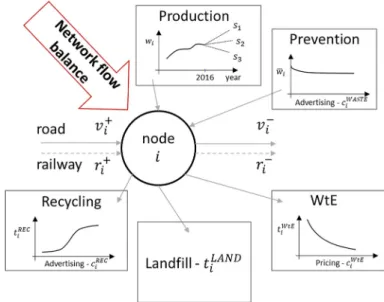
Fig. 1 General scheme of the proposed integrated system
uncertainty set (which can be seen as a support of the uncertain parameter) and the objective is to mitigate the impact of the worst-case possible. This approach is very well suited for the situations when the information about the uncertain parameters are limited (e.g. the lack of historical data), see Gulpinar et al. (2013) and Ben-Tal et al. (2009). Both Berglund and Kwon (2014) and Hu et al. (2017), however, consider only the box-budgeted uncertainty sets, which produce rather conservative solutions, but the resulting expressions remain linear (Ben-Tal et al.2009).
The novelty of this paper lies in several aspects. The mathematical model developed in Sect.2combines the pricing and advertising aspect in waste prevention and recy-cling, the facility location problem of new WtE plants, landfilling and WtE treatment options, and the design of a transportation network that uses both the road and rail transport options (see Fig.1for the illustration of the integrated system). The nonlinear (nonconvex) expressions that describe the effectiveness of recycling and prevention, and the cost of operating a WtE plant are linearized using SOS1 and SOS2 variables. Because of the scarcity of available data, the uncertainty is handled by robust optimiza-tion. However, the ellipsoidal uncertainty sets with varying immunization parameter are considered, as they more aptly capture the relationship between the uncertain parameters, without leaning toward the conservatism of the box-budgeted ones. The resulting mixed-integer second order cone problem is implemented inJuliaand a case study, demonstrating the usefulness of the method on a real-world example, is conducted (Sect.3).
2 Mathematical model
In this section, a robust mixed integer non-linear mathematical model for WM decision-making support is developed. The notation (Sect.2.1), constraints and objec-tive function (Sect.2.2), model linearization (Sect.2.3), uncertain waste production handling (Sect.2.4) and uncertainty incorporation (Sect.2.5) are subsequently pre-sented.
2.1 Notation used
Sets:
I set of all nodesi that form the network,i∈ I
J set of edgesj which connect nodes by road, j ∈ J⊆I×I L set of edgeslwhich connect nodes by railway,l∈ L⊆I×I. Parameters:
ai,j incidence matrix for road transportation
bi,l incidence matrix for rail transportation
ciL AN D cost for landfilling in the nodei
cW t Ei ,P E N penalty cost for energy and heat generation loss in WtE plant
cR O A Dj cost of transportation on road edge j
clR A I L cost of transportation on rail edgel
clR A I L,P E N penalization cost for railways
eiL AN D existing capacity of landfill in the nodei
mlR A I L lower bound for rail edgelwhen the edge is used
MlR A I L upper bound for rail edgel
mR O A Dj lower bound for road edge jwhen the edge is used
MR O A Dj upper bound for road edge j
ΔW t E possibility for prohibition of energy recovery in WtE plant
ΔL AN D possibility for prohibition of landfilling.
Decision variables:
eW t Ei designed capacity of WtE plant in the nodei
ri+ amount of waste transported to nodeiby rail
ri− amount of waste transported from nodeiby rail
tiL AN D amount of landfilled waste in the nodei
tiR EC amount of recycled waste in the nodei
tiW t E amount of processed waste in WtE plant in the nodei
vi+ amount of waste transported to nodeiby road
vi− amount of waste transported from nodeiby road
wi variable for the nominal waste production in the nodei
wi variable representing the waste production in the nodei
Fig. 2 Illustration of two dependencies: advertising-like and pricing functions
yl continuous variable representing the amount of flow on rail edgel
δl binary variable that indicates the activation of rail edgel
ωW t E
i amount of non-utilized capacity in the nodeiin WtE plant.
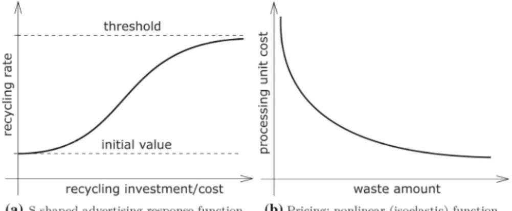
Besides the above mentioned parameters and decisions variables, the following (non-linear)cost functionsare considered. Note that two well-known marketing mech-anisms are presented—advertising and pricing (see Fig.2a, b)—and further used in the mathematical models.
cW t Ei (eiW t E) cost for processing in WtE plant (pricing)
cW AST Ei (wi)cost for reduction of waste produced (advertising-like)
ciR EC(tiR EC)cost for increasing of recycling (advertising-like).
2.2 Model description and formulation
The model developed in this section consists of (sets of) constraints (1)–(14) and one objective function (15).
2.2.1 Constraints
The constraint (1) forms the overall balance in the particular node. The amount of transported waste to the nodei(both means of transport – road, rail) and waste produced has to be equal to the amount transported from the nodeiand the waste treated (energy recovery, recycling, landfilling):
wi+vi++ri+=tiW t E+tiR EC+tiL AN D+vi−+ri− ∀i ∈ I. (1)
Constraints (2) and (3) define the rail transportation flows according to the incidence matrixbi,l and separate the amount of transported waste to (ri+) and from (ri−) the
l∈L:bi,l>0 bi,lyl =ri+ ∀i ∈I (2) l∈L:bi,l<0 −bi,lyl =ri− ∀i∈ I. (3)
Constraints (4) and (5) define the road transportation flows according to the inci-dence matrixai,jand separate the amount of transported waste to (vi+) and from (vi−)
the nodeirespectively:
j∈J:ai,j>0 ai,jxj =v+i ∀i∈ I (4) j∈J:ai,j<0 −ai,jxj =vi− ∀i ∈ I. (5)
In (6) and (7), the minimum and maximum flows are defined (when the edge is used) for all edges according to local infrastructure conditions for rail and road transportation respectively:
δlmlR A I L ≤yl ≤δlMlR A I L ∀l ∈L (6)
mR O A Dj ≤xj ≤MR O A Dj ∀j ∈ J. (7)
The Eq. (8) describes the utilization of designed capacities (eiW t E) for WtE plant in each nodei. ParameterΔW t E enables potential strategic decision which is to forbid the construction of WtE plants:
tiW t E+ωW t Ei =eW t Ei ΔW t E ∀i ∈ I. (8)
The constraint (9) limits the amount of landfilled wastetiL AN D byeiL AN D in the nodei. ParameterΔL AN D enables the prohibition of landfilling:
tiL AN D≤eiL AN DΔL AN D ∀i ∈ I. (9)
2.2.2 Constraints: domains of variables
All flows has to be non-negative for road and rail:
yl ≥0 ∀l∈ L (10)
xj ≥0 ∀j ∈ J. (11)
Transportation balance (rail, road) for waste out/in-flow for nodesi:
The amount of processed waste has to be non-negative for all waste treatment options, production, nominal production and penalized mount of waste in WtE:
eW t Ei ,tiW t E,tiR EC,tiL AN D, wi, wi, ωiW t E ≥0 ∀i∈ I. (13)
One more constraint is considered:
δl ∈ {0,1} ∀l ∈L. (14)
2.2.3 Objective function
The objective function (15) minimizes multiple transportation, processing and adver-tising costs: min l∈L ylclR A I L+ l∈L δlclR A I L,P E N + j∈J xjcR O A Dj + i∈I tiW t EciW t E(eW t Ei )+ i∈I ωW t E i c W t E,P E N i + i∈I cW AST Ei (wi) + i∈I tiR ECciR EC(tiR EC)+ i∈I tiL AN DciL AN D. (15)
The first row represents a transportation costs and edge operation fee for rail and road, respectively. The following summation defines the cost for processing in WtE plant. The next component penalizes the amount of non-utilized capacity representing the loss in heat and electricity generation. Costs of advertising to reduce the waste produced and to increase recycling follow. The last component summarizes cost for landfilled waste.
2.3 Linearization of the model
Costs associated with waste processing differ due to the type of facility. The price is fixed from a valid price list for operated landfills, but the price of WtE plant is depen-dent on its capacity (so-called pricing). This is described by non-linear function, which disrupt the model linearity and thus solvability. The same problem arises with recy-cling, which can be given by a logistic function or with waste production reduction (advertising). Properties of pricing and advertising functions (e.g., convexity) often results in difficulties with finding a global extreme. In addition, the problem is con-sidered as stochastic, which further complicates the situation. This huge non-linear problem can be solved by heuristic methods, but the optimality is not ensured and the computational time would also be enormous. This problem can be solved through the linearization of the application with piece-wise continuous linear function.
The linearization mentioned uses the so-called SOS1 and SOS2 variables (see Sect. 2.3.1). The SOS1 variables represent a set of mutually exclusive alternatives which can be chosen—this is used for the selection of the capacity of the WtE plant. The SOS2 variables are used for piece-wise linear approximation of the advertising
functions (at most two adjacent in the ordering given to the set can be non-zero and they must add up to 1, see Williams2009).
2.3.1 Additional notation and constraints
The next step is to provide new constraints for substitution of non-linearities in the model. The setK represents the set of pointskfor linearization (for eachk∈ K are defined values on horizontal and vertical axis). The following variables and parameters have to be defined.
SOS1 variables:
αW t E
i,k indicator of specific capacity of a WtE plant in node i.
SOS2 variables: αR EC
i,k specific investment indicator for recycling
αW AST E
i,k specific investment indicator for prevention of waste production.
Additional real variables: ˆ
tiW t E,k the amount of waste treated ati with capacity optionk
ˆ
ωW t E
i,k the amount of unused capacity atiwith capacity optionk.
Parameters:
ciR EC,k cost for recycled waste amount of linearization pointkin nodei
cW AST Ei,k cost for waste reduction of linearization pointkin nodei
cW t Ei,k cost for capacity of linearization pointkin nodeifor WtE plant
fiR EC,k advertising investmentkfor recycling in nodei
fiW AST E,k advertising investmentkfor waste reduction in nodei
fiW t E,k capacities for each linearization pointkfor WtE plant in nodei.
The constraint (16) acts in the same way as (8), linking the WtE treatment and unused capacity with the SOS1 variableαiW t E,k (this ensures that in each nodei the variablestˆiW t E,k ,ωˆiW t E,k can have nonzero values for only one optionk). The constraints (17), (18) and (19) link the WtE treatment, unused capacity and designed capacity in a nodei with the particular options (note that in these sums only one value can be nonzero). The Eqs. (20) and (21) are the SOS2 constraints for advertising in recycling and investments in waste reduction. The last constraint (22) enforces non-negativity of the additional variables.
ˆ tiW t E,k + ˆωiW t E,k =αiW t E,k fiW t E,k ΔW t E ∀i ∈ I,k∈K (16) tiW t E = k∈K ˆ tiW t E,k ∀i ∈ I (17) ωW t E i = k∈K ˆ ωW t E i,k ∀i ∈I (18) eiW t E= k∈K αW t E i,k fiW t E,k ∀i∈ I (19)
tiR EC = k∈K αR EC i,k f R EC i,k ∀i ∈ I (20) wi = k∈K αW AST E i,k fiW AST E,k ∀i ∈I (21) ˆ tiW t E,k ,ωˆiW t E,k ≥0 ∀i ∈ I,k∈K. (22)
2.3.2 Modified objective function
The modified objective function (23) reflects the newly defined linearization for pricing and advertising: min l∈L ylclR A I L+ l∈L δlclR A I L,P E N + j∈J xjcR O A Dj + i∈I k∈K ˆ tiW t E,k ciW t E,k + i∈I ωW t E i c W t E,P E N i + i∈I k∈K αW AST E i,k ciW AST E,k + i∈I k∈K αR EC i,k ciR EC,k + i∈I tiL AN DciL AN D. (23)
2.4 Handling the uncertainty: robust formulation and uncertainty sets
The only uncertainty in the data that is considered lies in the effect ofwi (the waste
production variable) on the real production. In other words, it is expected that the result of advertising for waste-reduction will be subjected to perturbationsζi (described
fur-ther). The question is how to come up with a sensible representation of this uncertainty. It is considered that historical data of waste production for all of the cities are available. For the purpose of this paper, the authors only have early data for the last 8 years, which is too few to come up with a useful time series/distribution estimation and construct a stochastic programming formulation (as in Gambella et al.2018). Instead, the methodology of robust optimization (Ben-Tal et al.2009) is used and the so-calleduncertainty setsare constructed, where the perturbations are expected. These uncertainty sets can be though of as the support of perturbation distribution, i.e., the smallest closed set so that the probability for the data to take a value outside of this set is zero. The resulting robust formulation will “immunize” the solution against the worst possible situation that may result from the selected uncertainty set.
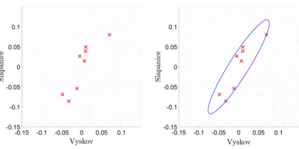
To come up with the uncertainty set, each pair of cities is examined first, look at the yearly fluctuations in production (see Fig.3a) and construct a minimal volume ellipsoid centered at zero, covering the fluctuations (see Fig.3b). The construction of the minimal volume ellipsoid (called the Löwner-John ellipsoid) covering finite set of points is done by solving the following problem (see Boyd and Vandenberghe2004). Let a zero centered ellipsoidEbe characterized as the inverse image of the Euclidean unit ball under an affine mapping:
Fig. 3 Construction of the pair-wise perturbation sets for the cities Vyškov and Šlapanice
It can be assumed w.l.o.g. thatUis a symmetric positive definite matrix (U∈Sn,U
0), in which case the volume ofEis proportional to detU−1. Having a finite set of pointsζ1, . . . , ζm ∈Rnthe problem can be written as follows:
min
U log detU
−1
s.t. ||Uζι||2≤1, ι=1, . . . ,m, U∈Sn, U0,
which is a convex (tractable) semidefinite program, that is solved using theSDPT3 solver within theCVXmodeling system (see Grant and Boyd2008) in theMATLAB programming language.
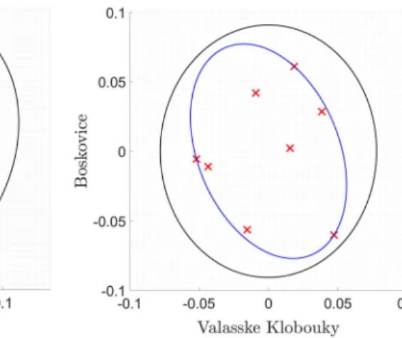
After computing these (N =561) covering ellipsoids (each having 2 dimensions), an additional ellipsoid (denoted asC= {ζ | ||Cζ||2 ≤1}) covering the union of the
pair-wise ones (in then =34 dimensions) is constructed. This step involves solving another convex semidefinite program of the following form:
min C,τ1,...,τN log detC−1 s.t. τ1≥0, . . . , τN≥0, C2−τιUι2 0 0 −1+τι 0, ι=1, . . . ,N, C∈Sn, C0,
which was solved, again, by using theSDPT3solver withinCVX. Note thatτ’s are auxiliary variables (Boyd and Vandenberghe2004). This covering ellipsoidCis mainly used in the evaluation of the obtained solutions. The projection ofCto a “pair-wise” plane can be seen in Fig.4.
Fig. 4 Projection of the covering ellipsoidC(black)
2.5 Incorporating the uncertainty
Let us identify the pair-wise ellipsoidal uncertainty derived earlier by the correspond-ing matrixU– that is the ellipsoidUi,ˆi will be used to denote the uncertainty set for citiesiandˆi ∈I. There are several options to incorporate these ellipsoidal uncertainty sets into the model. The first would be to use the following formulation:
⎡ ⎢ ⎢ ⎣1+ max ˆ i∈I,iˆ =i ξi,ˆi2≤Ω proji(Ui−,ˆi1ξi,ˆi) ⎤ ⎥ ⎥ ⎦wi ≤wi, ∀i ∈ I,
where projiis the projection to thei-th coordinate andΩdetermines the diameter of
the uncertainty set—settingΩ=1 results exactly in the ellipsoids derived previously, whereas smaller or larger values will shrink/enlarge the ellipsoids, but will not change their shape. SettingΩ =0 results in a “baseline” formulation, where no uncertainty is considered (the effect ofΩon the solution will be observed in Sect.3). The formulation above can be summarized by words as: “among all the ellipsoid that include cityifind the highest value in the corresponding coordinate”. The issue with this formulation is that it disregards the pair-wise structure of the uncertainty sets and results in an overly conservative solution.
Instead, the uncertainty sets will be incorporated by using the sums of pairs ofwi,
for which the structure is well-suited. The constraint has the form:
max ζi,ζˆi
Ui,ˆi[ζi;ζˆi]2≤Ω
which can be reformulated (see Ben-Tal et al.2009) as: wi+wiˆ+ΩU−1
i,ˆi [wi;wˆi]2≤wi+wiˆ, ∀i∈ I, ∀ˆi ∈ I, i = ˆi, (24)
which is a convex (tractable) second order cone constraint. To prohibit the solution from ending in extremely small or extremely large values forwi (which will happen
if,e.g., in a city the treatment costs are much smaller than in other ones), value ofwi
will be restricted by the maximum possible perturbation: ⎡ ⎢ ⎢ ⎣1+ max ˆ i∈I,ˆi =i ξi,ˆi2≤Ω proji(Ui−,iˆ1ξi,ˆi) ⎤ ⎥ ⎥ ⎦wi ≥wi, ∀i ∈I. (25)
3 Computations and results
The problem (1)–(14), (16)–(25) is a two-stage mixed-integer second-order cone pro-gramming problem. The first-stage (planning) variables include the decisions on nominal waste production wi, recycling tiR EC and designed capacity of the WtE
plantseiW t E. The rest of the variables (transportation and treatment) are considered second-stage (operational). Although this has no impact on solving the formulation, it influences how the solution will be evaluated. The solution will be evaluated on a test set of scenarios with different production perturbations. In the evaluation, only the first-stage variables are considered fixed by the solution and the second-stage variables are recomputed to minimize the costs (23), satisfying all the constraints. Furthermore, the solutions of (1)–(14), (16)–(25) for different values of the “immu-nization” parameter Ω are compared. To solve this problem, the JuMP modeling language (see, Dunning et al.2017) was used withinJuliafor modeling and the state-of-the-art solverGUROBI(Gurobi Optimization2016). The computations were performed on an ordinary machine (3.2 GHz i5-4460 CPU, 16 GB RAM).
3.1 Computational experiments on randomly generated networks
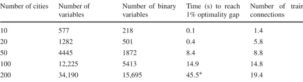
To give an insight into the computational tractability of the presented model, several instances of test networks were generated. The test networks were designed to roughly mimic the structure of the case study in all of the considered parameters. The instances contained 10, 20, 50, 100 and 200 cities, uniformly distributed on a square area, whose size was dependent on the number of cities. For example, the networks with 200 cities are on a square with a side length of 300 km—this setting approximates the geography of the Czech Republic, with 205 municipalities on the area of 78,865 km2. In each city, the waste production was between 250 and 380 kg per person, the recycling rate between 13% and 30%. The road network was constructed by connecting each city with its 5 nearest neighbors. The railroad network connected all cities that were between 60 and 200 km apart. For each city, 6 different WtE capacities/treatment costs were
Table 1 Results of the computational experiments, average values over 50 runs Number of cities Number of
variables Number of binary variables Time (s) to reach 1% optimality gap Number of train connections 10 577 218 0.1 1.4 20 1282 501 0.4 5.8 50 4445 1872 8.4 8.8 100 12,225 5413 14.9 14.8 200 34,190 15,695 45.5∗ 19.4
∗Only the instances that did not exceed the time limit
Fig. 5 Boxplot of the computation time to reach 1% optimality gap
considered. The investments into recycling and prevention were linearized by 6 and 11 SOS2 variables, respectively (with different values for each city, since the cities have varying “baseline” level of production and recycling).
Each instance was generated and solved 50 times (with a random value of the parameterΩ between 0 and 1), with optimality gap set to 1% and a time limit of 100 s. The results are summarized in Table1and Fig.5. The computational times are (maybe a bit unexpectedly) rather low. It is probably a combination of the incredible enhancements of the MIP solvers and hardware that took place in the last two decades (see, e.g., Bixby2012or Bertsimas2014) and a favorable structure of the optimiza-tion problem (as the SOS1 and SOS2 variables constitute a large part of the binary variables). For the problems with 200 cities, out of the 50 instances, 25 exceeded the time limit—the average optimality gap after the 100 s was 2.83%.
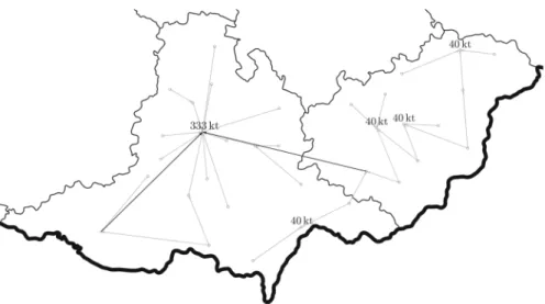
3.2 Case study
The problem instance of the case study investigated in this paper concerns two contigu-ous regions in the Czech Republic—the South Moravian Region and the Zlín Region, whose outline can be seen in Fig.6.
The problem has 4374 variables (of which 1818 are binary) and 3449 constraints (of which 561 are second-order cone). The number of variables is higher
com-Fig. 6 A map illustrating the solution forΩ=1. The numbers correspond to the installed capacities, black arrows indicate the use of the railroad and grey arrows the use of roads
pared to the randomly generated networks, because all possible railroad connections were considered. The optimality gap parameter was set to 0.01%, the computa-tions took less than 3 s. This problem was recomputed for 6 different values of Ω = [0,0.2,0.4,0.6,0.8,1](where the “baseline” case ofΩ = 0 does not con-tain any of the second-order cone constraints). One of the solutions (forΩ =1) is illustrated in Fig.6.
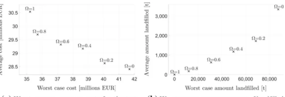
To evaluate the different solutions, 68 different scenarios of production pertur-bations were chosen. These scenarios correspond to the endpoints of the covering ellipsoidCin the direction of its principal axes (the eigenvectors of the corresponding matrixC). For these, the corresponding optimal second-stage (operational) variables were computed.
The results are best summarized in Fig.7. For all of the considered scenarios, the problem was feasible, indicating that the infrastructure (transportation network and waste treatment options) are robust enough (at least for the test cases). For higher values ofΩ, the worst-case costs over the test scenarios clearly outperforms the ones for lower values of Ω. However, the price for robustness of the solution is in its increased average costs (see Fig.7a)—the more “immunized” solutions tend to build more capacity for the WtE plans, which, in some scenarios, remains unused. The solutions with higher values ofΩ also tend to landfill much lower amounts of waste (see Fig.7b). In the end, it will be up to the actual decision-maker to choose the right balance between robustness against “unfortunate” fluctuations and possibly higher expected costs.
4 Conclusions and further research
The presented approach introduces several new modeling ideas in the area of WM and by the introduced model building and solving suggests new changes in the key
Fig. 7 The resulting costs and amount of landfilled waste. Evaluation for different values ofΩ
waste treatment infrastructure for the selected real-world case. The modeling follows the waste treatment hierarchy and locates the facility and its capacity. These relies on the pricing and advertising methods, which were included in the objective function. Relations were subsequently simplified using linearizations due to complexity reasons. The approach considers two different means of transport (road, rail) while both have its specific properties which influence the waste flow. The uncertainty was incorporated in the unknown future waste production through the ellipsoid based perturbations. The results are applicable to the area of waste treatment infrastructure planning and may serve as the support for the decision-makers to be robust enough and economically viable at the same time. The computational experiments suggest that the model is viable and tractable even for real-world problem instances. The original obtained solution may also be useful for analyzes dealing with all types of waste.
More specifically, the obtained results can be seen and analyzed from the perspec-tive of local authorities: apparently, a cooperation between particular regions seems justified. The results indicate that considering a low number of large-capacity WtE facilities with high heat demand is convenient; these can be accompanied with low-capacity WtE facilities that do not carry high risks of negative developments of waste availability. In large and complex problems, it is suitable to consider a combination of high capacity facilities accompanied by smaller regional projects. In the case of inter-regional transport, it is convenient to consider railway transport, which is envi-ronmentally friendly that helps with project acceptance by the population. Sensitivity analysis indicates that landfilling of a small amount of waste is a reasonable supple-ment from the economical point of view. Moreover, landfills bring a positive value regarding residues from the WtE facilities and so the overall eliminating of landfilling seems pointless. Last but not least, complex planning should not lead to planning of over-capacities that also cause high expenses of producers.
With respect to research limitations and our further research plans, it is important to emphasize that general modeling ideas that were specifically applied to the introduced real-world motivated problem can be modified and detailed for subsequent facility location and design problems in the area of sustainable development decision support, e.g. involving multistage decision making, see Gambella et al. (2018). Furthermore, the authors identified multi-objective approaches combining, e.g., costs, environmental
impact, residents mood, etc. as one of the potentially further research directions that the recent papers commonly propose (e.g., Eiselt and Marianov2014). Alternatively, as the waste production, priorities and strategies change, a dynamic location problem with an opening, closure and reopening of treatment facilities is possible (Dias et al.
2008). In case of better information on the data and on the correlation between the waste production in different cities, it would be possible to use a (possibly more efficient) stochastic programming approach (e.g., Gambella et al.2018).
Acknowledgements The authors gratefully acknowledge the financial support provided by the project Sus-tainable Process Integration Laboratory—SPIL, funded as project No. CZ.02.1.01/0.0/0.0/15_003/0000456, by Czech Republic Operational Programme Research and Development, Education, Priority 1: Strengthen-ing capacity for quality research. This work was also supported by the project “Computer Simulations for Effective Low-Emission Energy” funded as project No. CZ.02.1.01/0.0/0.0/16_026/0008392 by Operational Programme Research, Development and Education, Priority axis 1: Strengthening capacity for high-quality research. The author D. Hrabec further acknowledges project No. CZ.02.2.69/0.0/0.0/16_027/0008464 (International mobility of UTB researchers in Zlín) funded from the EU Funds—OP Research, Develop-ment and Education in cooperation with the Ministry of Education, Youth and Sports, Czech Republic.
References
Alçada-Almeida L, Coutinho-Rodrigues J, Current J (2009) A multiobjective modeling approach to locating incinerators. Socio-Econ Plann Sci 43:111–120.https://doi.org/10.1016/j.seps.2008.02.008
Allesch A, Brunner PH (2014) Assessment methods for solid waste management: a literature review. Waste Manag Res 32(6):461–473.https://doi.org/10.1177/0734242X14535653
Asefi H, Lim S (2017) A novel multi-dimensional modeling approach to integrated municipal solid waste management. J Clean Prod 166:1131–1143.https://doi.org/10.1016/j.jclepro.2017.08.061
Ben-Tal A, Ghaoui L, Nemirovski A (2009) Robust optimization. Princeton University Press, Princeton Berglund PG, Kwon C (2014) Robust facility location problem for hazardous waste transportation. Netw
Spat Econ 14:91–116.https://doi.org/10.1007/s11067-013-9208-4
Bertsimas D (2014) Statistics and machine learning via a modern optimization lens. (the 2014–2015 philip mccord morse lecture). INFORMS Annual Meeting, pp 1–42
Bing X, Bloemhof J, Ramos T, Barbosa-Póvoa A, Wong C, van der Vorst J (2016) Research challenges in municipal solid waste logistics management. Waste Manag 48(1):584–592.https://doi.org/10.1016/j. wasman.2015.11.025
Bixby R (2012) A brief history of linear and mixed-integer programming computation. Doc Math 19:107– 121
Blumenthal K (2011) Generation and treatment of municipal waste. Tech. Rep. KS-SF-11-031, Eurostat, European Commission: Luxembourg City, Luxembourg
Boyd S, Vandenberghe L (2004) Convex optimization. Cambridge University Press, Cambridge Corsini F, Gusmerotti N, Testa F, Iraldo F (2018) Exploring waste prevention behaviour through empirical
research. Waste Manag 79:132–141.https://doi.org/10.1016/j.wasman.2018.07.037
De Jaeger S, Rogge S (2013) Waste pricing policies and cost-efficiency in municipal waste services: the case of flanders. Waste Manag Res 31(7):751–758.https://doi.org/10.1177/0734242X13484189
Dias J, Captivo M, Cliímaco J (2008) A dynamic location problem with maximum decreasing capacities. Cent Eur J Oper Res 16(3):251–280.https://doi.org/10.1007/s10100-008-0055-1
Dunning I, Huchette J, Lubin M (2017) Jump: a modeling language for mathematical optimization. SIAM Rev 59(2):295–320.https://doi.org/10.1137/15M1020575
Eiselt H, Marianov V (2014) A bi-objective model for the location of landfills for municipal solid waste. Eur J Oper Res 235:187–194.https://doi.org/10.1016/j.ejor.2013.10.005
Eiselt H, Marianov V (2015) Location modeling for municipal solid waste facilities. Comput Oper Res 62:305–315.https://doi.org/10.1016/j.cor.2014.05.003
EPRS (2016) European parliamentary research service: circular economy package, online. URLhttp:// www.europarl.europa.eu/EPRS/EPRS-Briefing-573936-Circular-economy-package-FINAL.pdf
Gambella C, Maggioni F, Vigo D (2018) A stochastic programming model for a tactical solid waste man-agement problem. Eur J Oper Res.https://doi.org/10.1016/j.ejor.2018.08.005in press
Geissdoerfer M, Morioka S, Carvalho M, Evans S (2018) Business models and supply chains for the circular economy. J Clean Prod 190:712–721.https://doi.org/10.1016/j.jclepro.2018.04.159
Ghiani G, Lagana D, Manni E, Musmanno R, Vigo D (2014) Operations research in solid waste management: a survey of strategic and tactical issues. Comput Oper Res 44:22–32.https://doi.org/10.1016/j.cor. 2013.10.006
Grant M, Boyd S (2008) Graph implementations for nonsmooth convex programs. In: Blondel V, Boyd S, Kimura H (eds) Recent advances in learning and control, Lecture notes in control and information sciences. Springer, Berlin, pp 95–110
Gulpinar N, Pachamanova D, Canakoglu E (2013) Robust strategies for facility location under uncertainty. Eur J Oper Res 225:21–35.https://doi.org/10.1016/j.ejor.2012.08.004
Gurobi Optimization I (2016) Gurobi optimizer reference manual. URLhttp://www.gurobi.com
Hrabec D, Haugen K, Popela P (2017) The newsvendor problem with advertising: an overview with exten-sions. Rev Manag Sci 11(4):767–787.https://doi.org/10.1007/s11846-016-0204-1
Hu C, Liu X, Lu J (2017) A bi-objective two-stage robust location model for waste-to-energy facilities under uncertainty. Decis Support Syst 99:37–50.https://doi.org/10.1016/j.dss.2017.05.009
Inghels D, Dullaert W, Vigo D (2016) A service network design model for multimodal municipal solid waste transport. Eur J Oper Res 254:68–79.https://doi.org/10.1016/j.ejor.2016.03.036
Khouja M, Robbins SS (2003) Linking advertising and quantity decisions in the single-period inventory model. Int J Prod Econ 86:93–105.https://doi.org/10.1016/S0925-5273(03)00008-2
Lam H, Ng W, Ng R, Ng E, Aziz M, Ng D (2013) Green strategy for sustainable waste-to-energy supply chain. Energy 57:4–16.https://doi.org/10.1016/j.energy.2013.01.032
Martin J, Koralewska R, Wohlleben A (2015) Advanced solutions in combustion-based WtE technologies. Waste Manag 37:147–156.https://doi.org/10.1016/j.wasman.2014.08.026
McDougall F, White P, Franke M, Hindle P (2008) Integrated solid waste management: a life cycle inventory. Wiley, Hoboken
MECR (2014) Ministry of the environment of the Czech Republic: Waste management plan of the Czech Republic for the period 2015–2024, online
Tavares G, Zsigraiová Z, Semiao V (2011) Multi-criteria gis-based siting of an incineration plant for municipal solid waste. Waste Manag 31:1960–1972.https://doi.org/10.1016/j.wasman.2011.04.013
Williams H (2009) Logic and integer programming. Springer, London
Publisher’s Note Springer Nature remains neutral with regard to jurisdictional claims in published maps and institutional affiliations.