A flexible dependence model for spatial extremes
Jean-Noel Bacro †, Carlo Gaetan ‡, Gwladys Toulemonde† †IMAG, Universit´e de Montpellier, Montpellier, France
‡DAIS, Universit`a Ca’ Foscari - Venezia, Italy
Abstract
Max-stable processes play a fundamental role in modeling the spatial dependence of extremes because they appear as a natural extension of multivariate extreme value distributions. In practice, a well-known restrictive assumption when using max-stable processes comes from the fact that the observed extremal dependence is assumed to be related to a particular max-stable dependence structure. As a consequence, the latter is imposed to all events which are more extreme than those that have been observed. Such an assumption is inappropriate in the case of asymptotic independence. Following recent advances in the literature, we exploit a max-mixture model to suggest a general spatial model which ensures extremal dependence at small distances, possible independence at large distances and asymptotic independence at intermediate distances. Parametric inference is carried out using a pairwise composite likelihood approach. Finally we apply our modeling framework to analyze daily precipitations over the East of Australia, using block maxima over the observation period and exceedances over a large threshold.
1. INTRODUCTION
The last decade has registered a considerable effort to model extremes of data collected through a collection of sites and the interested reader is referred to Bacro and Gaetan (2012) and Davison et al. (2012) for recent reviews.
If the main interest is producing return level maps, the modeling issue is mainly concentrated on relating the parameters of the marginal distributions in each site to geographical covariates. In case of a residual dependence, uncertainty of the estimates can be further adjusted (Fawcett and Walshaw, 2007). Additionally, this modeling approach can be extended to be hierarchical adding a layer for incorporating spatial dependence through a spatial random process (Casson and Coles, 1999; Cooley et al., 2007; Gaetan and Grigoletto, 2007; Sang and Gelfand, 2010).
If we are interested in modeling the joint occurrence of extremes over a region, then the de-pendence structure of a multivariate variable needs to be explicitly stated. In this case the usual modeling strategy consists in two steps (1) estimating the marginal distribution and (2) character-izing the dependence via a model issued by the multivariate extreme value (MEV) theory (see for example Beirlant et al., 2004, and the references therein). These two steps can be integrated in a proper inferential analysis (Padoan et al., 2010; Ribatet et al., 2012).
The MEV theory deals with the tail behavior of a multivariate distribution from which we pretend that a sample is drawn and distinguishes three different forms of extremal dependence: asymptotic dependence, asymptotic independence and exact independence.
Asymptotic independence and dependence between a pair of random variables Z1 andZ2, with
marginal distributions F1 and F2, can be defined in terms of
χ= lim
u→1−Pr(F1(Z1)> u|F2(Z2)> u), (1)
whereχ= 0 and χ >0 represent asymptotic independence and dependence, respectively.
An example of a multivariate distribution which is asymptotically independent is given by the multivariate Gaussian distribution when the components are not perfectly correlated (Sibuya, 1960).
However the multivariate framework is inadequate for predicting or simulating values at un-observed sites. Therefore in the last years there was a general consensus in representing extreme spatial variability by max-stable processes (de Haan, 1984; Smith, 1990; Schlather, 2002; Kabluchko et al., 2009; Opitz, 2013) that are an infinite dimensional generalization of multivariate distributions for the maxima. The drawback of these processes is that they admit only two types of dependence
structures in their finite dimensional distributions: asymptotic dependence or exact independence. This restriction is constraining when we model the tail behavior of the multivariate distribution of the data because it is difficult to assess in practice whether a dataset should be modeled using an asymptotically dependent or asymptotically independent model (see Thibaud et al. (2013); Davison et al. (2013), for recent examples of these difficulties).
For coping with dependence structures that have not converged to their limiting form at ob-servable levels, Wadsworth and Tawn (2012) introduced the hybrid spatial dependence model. The
model originates from a max-mixture, namelyZ(s) = max(βX(s),(1−β)Y(s)) with 0≤β ≤1, of
an asymptotically dependent processX (a max-stable process, for instance), and an asymptotically
independent process Y.
In applications such as environmental ones different types of extremal dependencies could be present according the distance between two locations. As motivating example we shall consider winter daily cumulative rainfall, recorded at 31 monitoring sites in the East of Australia (Figure
3). We quantify the strength of the asymptotic dependence of a pair of random variablesZ(s) and
Z(s+h), located at sitessands+h, assuming the same marginal distributionF, by means of the
dependence measure (Coles et al., 1999)
χ(h, u) = 2−log Pr(F(Z(s+h))< u, F(Z(s))< u)
log Pr(F(Z(s))< u) , 0≤u≤1. (2)
In case of asymptotic independence,χ(u, h)'0 foru'1 andχ(h, u) is zero for exactly independent
variables for allu. Discriminating between asymptotic dependence and asymptotic independence by
means of the estimates ofχ(h, u) orχ(h), its limit version when u→1−, is not easy, especially for
rainfall extremes (Serinaldi et al., 2014). However the nonparametric estimates ofχ(h, u) (see Figure
5) suggest that asymptotic dependence is present up to a distancer1 and asymptotic independence
prevails for distances betweenr1 andr2 whereas for larger distances, exact independence could also
be conjectured (r1= 500 km and r2= 1000 km, approximately, in Figure 5).
In Wadsworth and Tawn (2012) the authors discuss the idea of having asymptotic dependence present up to a finite lag but in the reported examples asymptotic dependence or asymptotic independence are present for any distance, even if it is dimming with the distance. Following their idea, the contribution of the present paper is to consider examples of mixture between a max-stable process, that yields exact independence between maxima after a finite spatial lag and an asymptotically independent process that may or not yield exact independence between observations after that lag.
The max-stable process stems from the construction in Schlather (2002, p. 39) and, as example, we use the truncated Extremal Gaussian process (see also Davison and Gholamrezaee, 2012). For the asymptotically independent process we can consider stationary spatial processes with bivariate distributions satisfying only a general condition on the bivariate survivor functions (Ledford and Tawn, 1996, 1997). We exemplify our construction by means of a marginal transformed Gaussian process with possible finite range covariance function and of an inverse truncated Extremal Gaussian process.
The paper is organized as follows. In Section 2 we briefly introduce the max-stable and asymp-totically independent processes and some classical extremal dependence measures. Our modeling proposal and its main properties are detailed in Section 3 and a pairwise likelihood approach is presented for the statistical inference. In Section 4 we show, by means of a simulation study, that this approach seems effective in order to identifying different max-mixture models. Section 5 is devoted to illustrate the modeling issues related to our motivating example. Concluding remarks and some perspectives are addressed in Section 6.
2. SPATIAL EXTREMES MODELING
2.1 Models for asymptotic dependence
Max-stable processes (de Haan, 1984) are an infinite-dimensional generalization of multivariate
extreme value theory. The stochastic processX ={X(s), s∈ D}, whereD is a spatial domain, is
a max-stable process if and only if there exist functions an(·)>0 andbn(·) onR such that
max 1≤i≤n Xi(s)−bn(s) an(s) d =X(s)
where X1, X2, . . . are independent copies of X. In the sequel and without loss of generality, D is
a subset ofR2 and univariate margins of max-stable processes are assumed to be unit Fr´echet, i.e.
Pr(X(s)≤x) = exp(−1/x), x >0.
A max-stable process has a spectral representation (de Haan, 1984; Schlather, 2002). Assume
that ri, i≥1, are points of a Poisson process on (0,∞) with intensity dr. Let Wi, i≥1, be
independent and identically distributed (iid) copies of a real valued continuous random function
W = {W(s), s ∈ D}, independent of the {ri} and such that E[W+(s)] = µ ∈ (0,∞), where
W+(s) = max(W(s),0). Then
X(s) =µ−1max
i≥1 W +
i (s)/ri (3)
Choosing a particular expression for Wi leads to known examples of max-stable processes: the
Gaussian extreme value process (Smith, 1990), the extremal Gaussian process (Schlather, 2002),
the Brown-Resnick process (Kabluchko et al., 2009) and the extremaltprocess (Opitz, 2013).
In the sequel we focus on a particular instance of a max-stable process: the Truncated Extremal Gaussian (TEG) process. The TEG process has been introduced by Schlather (2002) and has been exemplified by Davison and Gholamrezaee (2012). As in the extremal Gaussian model the model derives from an underlying Gaussian process censored on a compact random set.
Let ri,i≥1, be defined as previously and consider Wi(s) =cmax(0, εi(s))1IBi(s−Ui) with εi
independent copies of a stationary Gaussian processε={ε(s), s∈ D}with zero mean, unit variance
and correlation functionρ(·), 1IBis the indicator function of a compact random setB ⊂ D, of which
Bi are independent replicates and Ui are points of a homogeneous Poisson process of unit rate on
D, independent of the εi. Choosing the constantc such thatc−1 =E(max{Wi(s),0}1IBi(x−Ui)),
the TEG process is defined as
X(s) = max
i≥1
Wi(s)
ri . (4)
The marginal distribution of X is unit Fr´echet and the bivariate one is given by
Pr (X(s)≤t1, X(s+h)≤t2) = exp −t11 + 1 t2 1− α(h) 2 1−1−2(ρ(h)+1)t1t2 (t1+t2)2 1/2 (5) whereα(h) =E[|B∩(h+B)|]/E[|B|]. IfB is a disk of fixed radiusr,α(h) can be approximated by
α(h)'(1− ||h||/(2r)) 1I[0,2r](||h||). (6)
2.2 Models for asymptotic independence
A multivariate vector is asymptotically independent (AI) if and only if all its pairs of components are AI (de Oliveira, 1962). As a consequence, if all the bivariate distributions of a stochastic process are AI, the stochastic process is said to be AI.
For modeling AI we assume a specific model for bivariate joint tails as described in more detail in Ledford and Tawn (1996).
We assume that{Z(s), s∈ D}is a stationary spatial process with unit Fr´echet margins. Under
weak conditions, Ledford and Tawn (1997, 1998) showed that the bivariate tail distribution of a
pair of observations at sand s+h admits an approximation such that
Pr(Z(s)> z1, Z(s+h)> z2)∼z−
c(1)h
1 z −c(2)h
for z1 and z2 simultaneously large, where 0 < 1/(ch(1)+c(2)h ) ≤ 1 and L0h 6= 0 a bivariate slowly
varying function (Bingham et al., 1987, Appendix 1) with limit functiongh such that for allx >0,
y > 0 and c > 0, gh(x, y) = lim
t→∞L 0
h(tx, ty)/L0h(x, y) and gh(cx, cy) = gh(x, y). The homogeneity
property of gh implies that gh(x, y) = g∗h(w) with w = x/(x+y) ∈ [0,1] where the function gh∗,
often called the ray dependence function, is assumed to be a slowly varying function at 0 and 1.
Assuming z1 =z2 =z leads to the Ledford-Tawn (LT) model for bivariate joint tails (Ledford
and Tawn, 1996):
Pr(Z(s)> z, Z(s+h)> z)∼z−1/η(h)Lh(z) forz→ ∞ (7)
whereLh(·) is a univariate slowly varying function. The coefficientη(h) varies between 0 and 1 and
determines the decay rate of the bivariate tail probability Pr(Z(s)> z, Z(s+h) > z) for large z.
Despite its simplicity, equation (7) appears as a very general model for bivariate joint tails which
can provide, as detailed below, a measure of the extremal dependence between Z(s) and Z(s+h)
through the coefficientη(h). Asymptotic independence corresponds toη(h)<1 and in such a case,
η(h) measures the degree of dependence in the asymptotic independence at h, where η(h) >1/2
and η(h) <1/2 indicate positive and negative association, respectively. When the variablesZ(s)
andZ(s+h) are independentη(h) = 1/2. There are few examples of AI processes in the literature.
In the sequel three asymptotically independent processes are considered with explicit expressions of (7).
Example 1: Stationary Gaussian process
Let{Y(s), s∈ D}be a stationary Gaussian process with zero mean, unit variance and correlation
function ρ(h). Because bivariate Gaussian variables are AI provided that they are not perfectly
correlated (Sibuya, 1960), the spatial process Z0(s) =−1/log(Φ(Y(s))) has unit Fr´echet margins
and verifies (Ledford and Tawn, 1996)
Pr(Z0(s)> z, Z0(s+h)> z)∼Chz−2/{1+ρ(h)}(logz)−ρ(h)/{1+ρ(h)}
withCh = (1 +ρ(h))3/2(1−ρ(h))−1/2(4π)−ρ(h)/{1+ρ(h)}. Soη(h) ={1 +ρ(h)}/2.
Example 2: Inverse max-stable process
The inverse max-stable process (Wadsworth and Tawn, 2012) is obtained by simply inverting a
max-stable process. More precisely, let {X(s), s ∈ D} be a max-stable process defined as in (3).
Then the process
is an AI process with Fr´echet margins. For any fixed h, the tail dependence coefficient is η(h) =
1/θ(h) whereθ(h) is the extremal coefficient of the max-stable process.
Example 3: Max-Gaussian ratio process
Recently Padoan (2013) introduced a new family of spatial processes whose univariate limit dis-tributions are unit Fr´echet and bivariate disdis-tributions are able to cope with different levels of dependence according to the magnitude of extreme events. Such processes, called max-Gaussian ratio processes, are obtained as pointwise maxima of samples from a ratio of Gaussian processes
with common correlation function. For every n ∈ N, let {Un(s), s ∈ D} and {Vn(s), s ∈ D} be
two independent Gaussian processes on D with mean zero, unit variance and common correlation
function, ρn(h), such that
ρn(h) = 1−
λ(h)2
2n2 +o n−
2, as n→ ∞
Hereλ(h)>0 forkhk 6= 0. Assume also thatYi,n(s) are independent copies ofYn(s) =Un(s)/Vn(s)
and define Mn(s) = maxi=1,...,nYi,n(s). Then the normalized bivariate asymptotic distribution of
(Mn(s), Mn(s+h)) is Pr(W(s)≤w1, W(s+h)≤w2)≡ lim n→∞Pr(Mn(s)≤ nw1 π , Mn(s+h)≤ nw2 π ) = exp −Vλ(h)(w1, w2) where Vλ(h)(w1, w2) = 1 2 2 w1 + 2 w2 +λ(h) + s 1 w1 − 1 w2 2 +λ(h)2− s 1 w12 +λ(h) 2− s 1 w22 +λ(h) 2 . For a given λ(h), Pr(W(s)> w, W(s+h)> w)∼ 1 + 1 2λ(h) w−2 as w→ ∞
leading to a constant tail dependence parameter η(h) = 1/2. As underlined by Padoan (2013), a
general framework based on equation (7) allows for different speeds of convergence to the indepen-dence case and could be used for depenindepen-dence structures with a slower convergence than that of max-Gaussian ratio processes.
2.3 Pairwise extremal dependence measures
We recall here some measures of extremal dependence for spatial processes. From a theoretical point of view, the dependence structure of any multivariate extreme distribution is characterized by the exponent measure (see Resnick, 1987, for example). Unfortunately, it is quite difficult to infer this
measure from the data. That is why summaries of extremal dependence based on pairwise measures
have been proposed (Coles et al., 1999). For a stationary spatial process Z ={Z(s), s∈ D} with
univariate cumulative distribution functionF, the pairwise extremal dependence between two sites
sand s+hcan be characterized using the function
χ(h) = lim
u→1−Pr(F(Z(s+h))> u|F(Z(s))> u)
since we have pairwise asymptotic independence or asymptotic dependence (AD) if and only if
χ(h) = 0 orχ(h)6= 0, respectively (Sibuya, 1960). Alternativelyχ(h) can be expressed as limit for
u→1− of χ(h, u), defined in (2). The function χ(h,·) can be interpreted as a quantile-dependent
measure of dependence between two sites separated byh, giving more insight ifZ(s) andZ(s+h)
are positively or negatively associated (Coles et al., 1999). Note also that for a max-stable process
any bivariate distribution is max-stable and then the functionχ(h, u) is constant with respect tou
for a fixedh.
The extremal coefficient function (Schlather and Tawn, 2003) is a specific measure of the
de-pendence for a max-stable process X. Given a pair of sites s and s+h the extremal coefficient
functionθ(h) is defined as
Pr(X(s)≤x, X(s+h)≤x) = Pr(X(s)≤x)θ(h).
Here 1≤θ(h)≤2 and θ(h) = 1 orθ(h) = 2 corresponds to perfect dependence or exact
indepen-dence, respectively. It is easy to show thatθ(h) = 2−χ(h).
Special instances of the Gaussian extreme value process (Smith, 1990) or the Brown-Resnick process (Kabluchko et al., 2009) span the range of possible extremal dependencies from perfect
dependence to exact independence provided that distance khk increases indefinitely. Instead the
extremal Gaussian process (Schlather, 2002) cannot account for extremes that become independent after some distance. Note that the TEG process has the feature that its extremal coefficient function
θ(h) = 2−α(h)n1−2−1/2[1−ρ(h)]1/2o (8)
reaches the upper value (θ(h) = 2) for ||h|| large enough. This specific feature will be exploited
later.
Under asymptotic independence, bothχ(h) andθ(h) functions are uninformative and of limited
interest. Assume again thatZis a stationary spatial process with univariate cumulative distribution
functionF, and define
¯
χ(h, u) = 2 log Pr(F(Z(s))> u)
The limit ¯χ(h) = limu→1−χ¯(h, u), with −1 <χ¯(h) ≤ 1, provides another measure that increases
with the extremal dependence between Z(s) and Z(s+h) (Coles et al., 1999). It turns out that
for AD process ¯χ(h) = 1, for all h. Moreover under the condition (7), it is easy to show that
¯
χ(h) = 2η(h)−1 and the tail dependence coefficientη(h) appears as another dependence measure
of interest (Ledford and Tawn, 1996, 1997; Ancona-Navarrete and Tawn, 2002).
Note that the empirical estimate of (9) provides an useful statistic for inspecting the tail behavior
when u <1. For the stationary Gaussian process with correlation function ρ(h) we can show that
¯
χ(h, u) varies with u (Coles et al., 1999, p. 348) with limit ¯χ(h) =ρ(h) andη(h) = (1 +ρ(h))/2.
For the inverse max-stable process, ¯χ(h,·) is a constant function. In other words, bivariate survival
distributions of inverse max-stable processes are uniquely linked to the marginal survival function
of the process whatever the magnitude of the considered extreme events. Moreover we have ¯χ(h) =
2/θ(h)−1.
Finally, the function ¯χ(h, u) of a max-Gaussian ratio process varies with u and tends to 0 as
u→1− for a fixed value ofλ(h).
3. MAX-MIXTURE MODELING OF SPATIAL EXTREMAL DEPENDENCE
3.1 Model specification
Let X = {X(s), s ∈ D} and Y ={Y(s), s∈ D} be two independent stationary spatial processes,
such thatX is a max-stable process andY an AI process both with unit Fr´echet univariate
distri-butions. We define the max-mixture (MM) model as
Z(s) = max(βX(s),(1−β)Y(s)), 0≤β ≤1. (10)
The MM model has been introduced by Wadsworth and Tawn (2012) for modeling situations where the extremal dependence structure may vary with distance. Even if it is not max-stable process, the MM model allows a different order of decay towards an asymptotically dependent limit which
inherits the same dependence structure of X. In Wadsworth and Tawn (2012) various instances of
max-stable processes along with their inverted versions as AI processes have been considered and all fitted models had asymptotic dependence or asymptotic independence present at all spatial lags. Owing to our motivating data set, we propose in the sequel to extend the set of examples by considering a max-mixture model that deals with asymptotic dependence at short lags, asymptotic independence at intermediate lags and possibly exact independence at larger lags. More precisely
examples in Wadsworth and Tawn (2012), we broaden the class of considered AI processes by taking into account AI processes with unit Fr´echet univariate distributions and bivariate distributions
satisfying the LT model (7) forη(h)<1.
Using the independence between the two processes X andY it is straightforward to obtain the
bivariate distribution for a pair of sites, namely Pr(Z(s)≤z1, Z(s+h)≤z2) = exp −βz1 1 + 1 z2 1− α(h) 2 1−1−2(ρ(h)+1)z1z2 (z1+z2)2 1/2 Fh Y z1 1−β,1z−2β (11) where FYh(y1, y2) = Pr(Y(s) ≤y1, Y(s+h) ≤y2). Since Pr(Z(s) ≤z) = Pr(Z(s)≤z, Z(s+h)<
∞) = exp (−1/z) the model has unit Fr´echet univariate distribution.
3.2 Pairwise extremal dependence measures of the model
Exploiting characterization (7), the bivariate tail distribution of (10), for largez, can be expressed
as: Pr(Z(s)> z, Z(s+h)> z) = β(2−θ(h)) z + z 1−β −1/η(h) Lh z 1−β +O(z−2).
So it is easy to deduce theχ(h) function using equation (8), namely
χ(h) =β(2−θ(h)) =β α(h) 1− r 1−ρ(h) 2 ! .
If the approximation (6) holds, it turns out that pairs of sites separated by a distance||h||are AD
if this distance is smaller than 2r and AI otherwise.
For evaluating ¯χ(h), we need to evaluate the logarithm of the bivariate tail distribution. We
obtain log Pr(Z(s)> z, Z(s+h)> z) =
log (β(2−θ(h)))−logz+o(log(z)) if 2−θ(h)6= 0
−η(h)−1log1−zβ+ logLh z 1−β +o(1), otherwise
If 2−θ(h) 6= 0, we can conclude that ¯χ(h, z) →1 as z→ ∞. On the other hand, if 2−θ(h) = 0,
we have ¯ χ(h, z)∼ −2− zlog2 z −η(1h)(1− log(1−β) logz ) + log(Lh(z/(1−β))) logz −1,
i.e. ¯χ(h, z)→2η(h)−1 asz→ ∞. Owing to (6) the results can be summarized into the formula
¯
that highlights the different behaviour according to the distance between two sites. Let R > 2r
and assume that η(h) = 1/2 for ||h|| > R. Then pairs of sites separated by a distance ||h|| are
asymptotically dependent for ||h|| < 2r, asymptotically independent for 2r ≤ ||h|| ≤ R and near
independent for||h||> R. For example, for the transformed stationary Gaussian process with unit
Fr´echet margins and correlation function ρY(h), we have:
¯
χ(h) = 1I[0,2r](||h||) +ρY(h)1I[2r,∞)(||h||).
In that case, independence is achieved if the correlation functionρY(·) is such thatρY(h) = 0 when
||h||> R.
3.3 Model inference
For the model (10) since the full likelihood is intractable to evaluate, a composite likelihood ap-proach is used for parametric estimations using pairs. The composite likelihood is an inference function derived by multiplying likelihoods of marginal or conditional events (Lindsay, 1988; Varin, 2008). Such an approach has been applied in spatial extremes using bivariate densities of max-stable processes (Padoan et al., 2010) or bivariate density of exceedances over a large threshold (Jeon and Smith, 2012; Wadsworth and Tawn, 2012; Bacro and Gaetan, 2014; Huser and Davison, 2014). Recently, improvements have been obtained for the parameters estimations of some max-stable processes, e.g. Brown-Resnick processes: extremal increments of the process allow to work with a complete likelihood function (Engelke et al., 2015; Wadsworth and Tawn, 2014). A direct modeling of the exceedances of a max-stable process is also possible using a generalized Pareto pro-cess (Ferreira and de Haan, 2014) but such an approach is only of interest in the case of asymptotic dependence.
If zik is the site-wise block maximum, for instance seasonal maximum, observed at site si,
i= 1, . . . , N and at timetk,k= 1, . . . , M, the pairwise (weighted) log-likelihood is defined by
pl(ψ) = M X k=1 plk(ψ) = M X k=1 NX−1 i=1 N X j>i wijlogL(zik, zjk;ψ) (12)
whereL(zik, zjk;ψ) is the likelihood of a pairzik, zjk, The weightswij are non negative and specify
the contributions of each pairs. A simple weighting choice is to let wij = 0 for any pair whose
distance exceeds a specified valueδ, and let wij = 1, otherwise.
Recently Wadsworth and Tawn (2012) argued that, under asymptotic independence, it is more
proposal the pairwise likelihood contribution L(zik, zjk;ψ) becomes L(zik, zjk;ψ) = ∂2 ∂zik∂zjkG(zik, zjk;ψ) if max(zik, zjk)> u G(u, u;ψ) if max(zik, zjk)≤u (13)
wherezik is the observed value and G(·,·) designates the bivariate distribution (11).
When dealing with exceedances it is not reasonable to assume that the observations are
indepen-dent over the time. Assuming that the space-time process is temporallyαmixing, the function (12)
is a contrast function and conditions in Guyon (1995, Theorem 3.4.7) are satisfied. Thus the
max-imum composite likelihood estimatorψbis asymptotically Gaussian for largeM and its asymptotic
variance is given by the inverse of the Godambe information matrix G(ψ) =H(ψ)[J(ψ)]−1H(ψ).
Standard error evaluation requires consistent estimation of the matricesH(ψ) =E(−∇2pl(ψ)) and
J(ψ) =Var(∇pl(ψ)).
It is worth noting that such results hold if the data are actually from the limit model and this fact can add a bias (for an accurate study see Jeon and Smith (2012)) and, consequently, further uncertainty in the estimates.
The matrix H(ψ) can be estimated byHb=−∇2pl(ψb
T). Estimation of the matrix
J(ψ) = M X k=1 M X k0>k Cov∇plk(ψ)∇plk0(ψ)0
requires some care when we deal with temporally dependent data. In this paper we estimate J
by means of a subsampling technique (Carlstein, 1986). More precisely, we considerB overlapping
blocks Db ⊂ {1, . . . , M},b= 1, . . . , B, of size db and the estimate
b J = M B B X b=1 1 db∇ plDb(ψb)∇plDb(ψb)0
whereplDb is the pairwise likelihood evaluated over the blockDb.
Finally we mention that an appropriate model selection criterion to the pairwise likelihood is the composite likelihood information criterion (Varin and Vidoni, 2005), namely
CLIC =−2hpl( ˆψ)−tr{Hˆ−1J }ˆ i.
Lower values of CLIC indicate better fit.
4. SIMULATION STUDY
To assess the quality of the estimation procedure in case of the MM model (10), a simulation study
r and exponential correlation function ρ(h) = exp(−khk/ρ1), ρ1 > 0. The asymptotically
inde-pendent process,Y, is given byY(s) =−1/log((Φ(Y0(s))), where Φ is the cumulative distribution
function of a standard normal distribution and {Y0(s), s ∈ D} is a Gaussian spatial process with
spherical correlation function, i.e. 1−1.5(khk/ρ2) + 0.5(khk/ρ2)3, for khk ≤ ρ2, zero otherwise,
ρ2 >0.
Under this setup extreme observations at sites separated by a vector h are asymptotically
dependent if khk < r, asymptotically independent if r ≤ khk < ρ2 and independent if khk ≥ ρ2,
provided that r < ρ2.
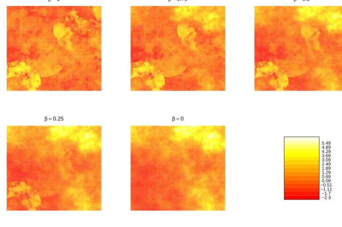
Five simulated images of the MM model over the [0,1]2 square are shown in Figure 1, according
to different values of the mixing parameterβ. Actually, in order to appreciate the role of the mixing
parameter β, the values in the images are derived by considering the simulation when β = 0 (AI
process) andβ = 1 (AD process). Note that the degree of smoothness decreases withβ.
In the simulation study we have considered a moderately sized dataset with N = 49 sites and
M = 1000 independent observations. To avoid too systematic distances between pairs of sites, a
non regular spatial grid has been considered. The [0,1]2square is divided into 49 equal sub-squares
and within each sub-square a point is uniformly chosen at random. We set ρ1 = 0.2,ρ2 = 0.8 and
r= 0.25 and different values of β ∈ {0,0.25,0.50,0.75,1}.
The parameters are estimated on 500 data replication using the composite likelihood approach
detailed in Section 3.3. The threshold u is taken corresponding to the 0.9 empirical quantile at
each site and theδ value is chosen as the 0.9 quantile of the distribution of the distances between
pairs of sites.
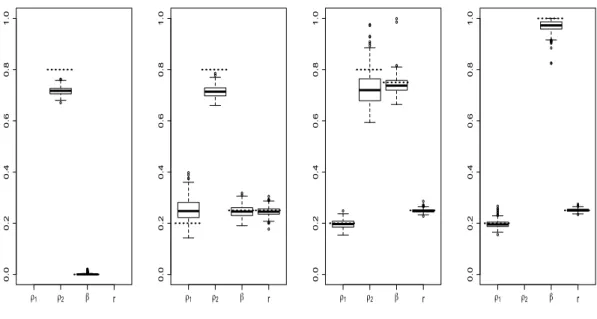
For compactness we report only the results for 500 data replications with β = 0,0.25,0.75,1.
For β = 0.5 we have obtained similar results. The boxplots in Figure 2 show that, overall, the
parameters are well estimated except ρ2 the parameter of the spherical correlation for which the
estimate is significantly biased. This inadequacy seems consistent with the difficulties in estimating the parameter of the spherical correlation function in Gaussian models (Mardia and Watkins, 1989). In our example a justification for choosing a spherical correlation function is to consider a
potential extremal exact independence for distances larger thanρ2. Simulations with an exponential
correlation function not reported here lead to unbiased estimates of the range parameter.
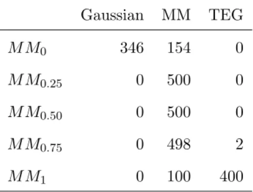
Thereafter, we assessed whether CLIC is useful in identifying the true model, i.e. in our frame-work if we can use CLIC for discriminating between asymptotic independence, asymptotic
depen-dence or a mixture of this. We have considered 500 simulations from mixture models with the same setting as before. In Table 1 we summarize our findings that are quite encouraging. We denote
by MMβ, β ∈ {0,0.25,0.50,0.75,1} the MM model according to different values of the mixing
parameter. When the simulations come from MMβ, β = 0.25,0.5 and 0.75, identification based
on minimizing the CLIC value performs extremely well. Moreover the proportion of simulations
in which the true model is detected is 68.6% if the true model is the AI process (MM0). This
proportion increases to 80% when the TEG process (β = 1) is the true model.
Gaussian MM TEG M M0 346 154 0 M M0.25 0 500 0 M M0.50 0 500 0 M M0.75 0 498 2 M M1 0 100 400
Table 1: Number of identified models according CLIC under different M Mβ model, β ∈
{0,0.25,0.50,0.75,1} withρ1 = 0.2,ρ2= 0.8,r = 0.25.
5. REAL DATA EXAMPLE
We analyze daily rainfall data from the 31 stations in the East of Australia whose locations are shown in Figure 3. The values come from the daily rainfall dataset of Lavery et al. (1992), available
at time of writing atftp.bom.gov.au/anon/home/ncc/www/change/HQdailyR.
Daily rainfall totals are for the 24-hours (measured at 9am) and we consider days in the winter period (April – September) for 49 years ranging from 1955 to 2003.
Empirical estimates of the functions χ(h, u) and ¯χ(h, u) can be constructed on the basis of
observed data by using the empirical estimates of univariate and bivariate distributions. In order to explore possible anisotropy of the dependence we have plotted (Figure 4) the loess smoothing
of ˆχ(h, u) and ˆχ¯(h, u) at u = 0.975 with respect to the distances in different directional sectors,
namely (−π/8,π/8], (π/8,3π/8], (3π/8, 5π/8], (5π/8, 7π/8], where 0 represents the northing
direc-tion. Based on these estimates there is no clear evidence of anisotropy even if a stronger spatial dependence appears in the Northing direction.
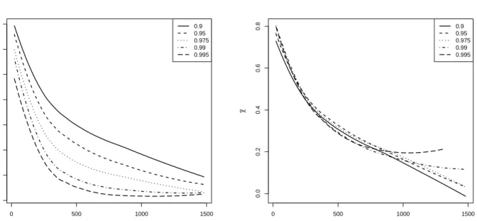
Moreover, as we mentioned in the introduction, the isotropic estimates (Figure 5) of the
between sites seems to be present up to a distance of 500 km, and asymptotic independence could be conjectured between 500 km and 1000 km distances. Therefore a max-mixture model seems a good candidate for interpreting the extreme value dependence. However the strength of dependence decreases when considering exceedances of increasing thresholds. This fact highlights the difficulty in a proper modeling of the asymptotic dependence for short distances.
In the sequel, we shall consider seven models that belong to three classes: mixture, max-stable and asymptotically independent. Each model is fitted using a subset of 16 sites and the remaining sites are used to perform model validation. We shall consider three MM models, namely
A1 a MM model (10) specification in which X is a TEG process with exponential correlation
function exp{−khk/ρ1}, ρ1 > 0 and B1 is a disc of fixed and unknown radius r1. The
asymptotically independent process is given by Y(s) = −1/log((Φ(Y0(s))), where Φ is the
cumulative distribution function of a normalized Gaussian random variable andY0is a
Gaus-sian spatial process with spherical correlation function 1−1.5(khk/ρ2) + 0.5(khk/ρ2)3, for
khk ≤ρ2, zero otherwise,ρ2>0;
A2 a MM model (10) where X is a TEG process as inA1 and Y0 is a Gaussian spatial process
with exponential correlation function exp{−khk/ρ2};
A3 a MM model with the sameX as specified in A1 and A2 and in whichY is an inverse TEG
process with exponential correlation function exp{−khk/ρ2},ρ2>0. TheB2 disc has a fixed
and unknown radiusr2.
As max-stable model candidate, we consider a max-stable model that entails exact independence
between sites after a distance greater than 2r1, i.e.
B the TEG process specified inA1.
Finally we take into account three asymptotically independent models, namely
C1 the asymptotically independent process specified asY inA1;
C2 the asymptotically independent process specified asY inA2;
C3 the asymptotically independent process specified asY inA3.
Note that models C1 and C3 result in exact independence after distances greater thanρ2 and
5.1 Site-wise maxima
First of all we have considered model site-wise winter maxima. Model (10) assumes common marginal Fr´echet distributions and a proper inferential approach requires to fit marginal and depen-dence parameters. However, because we are interested in the appropriateness of different degrees of spatial asymptotic dependence, we prefer to follow a more simple and pragmatic approach. Specif-ically, we fit separately a GEV distribution in each site and we use the estimates to transform the marginals to unit Fr´echet. The dependence parameters are estimated using the pairwise likelihood approach. Padoan et al. (2010) found in their simulation study that relatively small values of the
distance δ in (12) produces gains in computation efficiency as well as in statistical efficiency of the
estimates. However in our case we prefer to setδ '1000 km, which entails to consider about 90%
of all distinct observational pairs. For evaluating the CLIC and the standard errors we assume
that the seasonal maxima are independent. In that case the estimation of the matrixJ is greatly
simplified in the subsampling procedure and we have considered M = 49 non overlapping blocks
Db corresponding to a single year , i.e. db= 1.
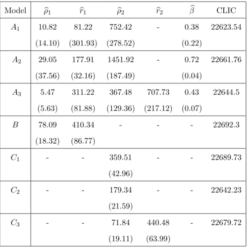
Our findings are summarized in Table 2. The rather wide standard-error of the spatial param-eters, in particular for the max-mixture models, probably can be justified by the small number of independent replications over the years, pointing out that it is hard to separate the contribution
of the components in the max-mixture. As suggested by the CLIC, the best-fitting model is A1,
for which pairs of sites separated by a distance d smaller than 160 km or greater than 750 km
are asymptotically max-stable dependent or exactly independent, respectively. At intermediate distances the seasonal maxima exhibit asymptotic independence. Moreover according to the CLIC values the MM models and the asymptotic independence models appear superior to the max-stable
model B. So the max-stable model seems to overestimate the level of dependence in the data.
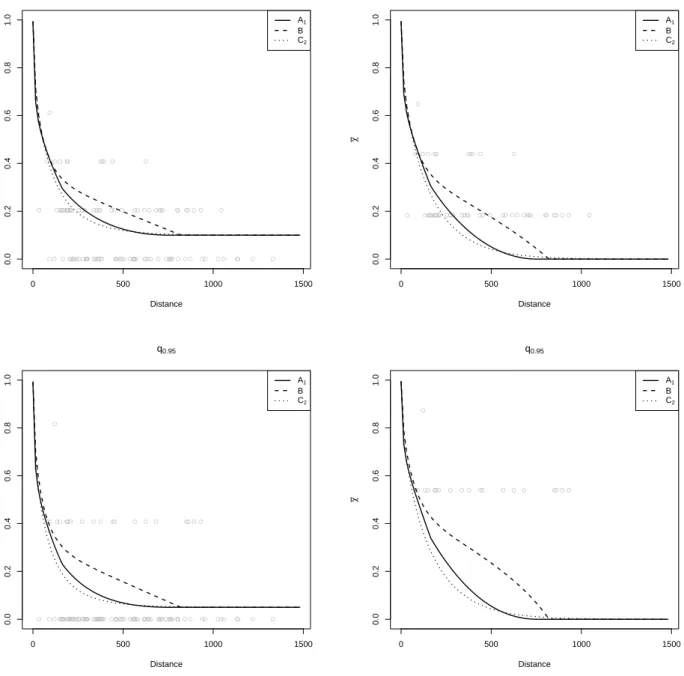
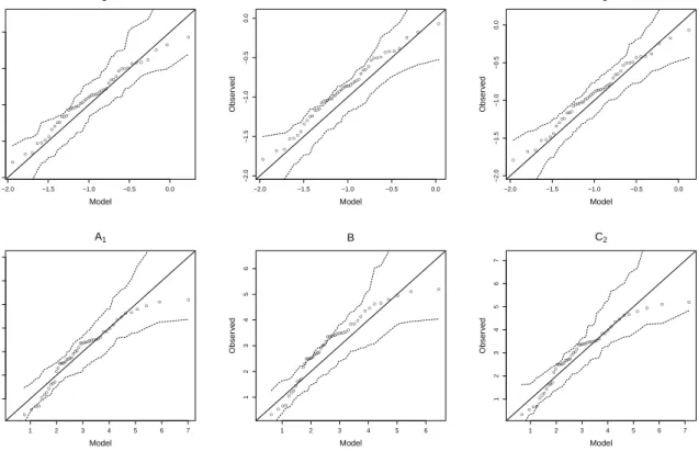
The goodness of fit has been also assessed in two different ways. Figure 6 shows the empirical
values for χ(h, u) and ¯χ(h, u), with u = 0.9 and 0.95 and their model-based counterparts of the
three best models in each class according to the CLIC. Empirical estimates are calculated on the
validation data set. The fits at finite thresholds are similar forA1 andC2 and the max stable model
B entails stronger dependence for any distance. Considering the general patterns and owing to the
small number of repeated observations for each site it is difficult to see which model catches better the bulk of the empirical values.
Model ρb1 br1 ρb2 br2 βb CLIC A1 10.82 81.22 752.42 - 0.38 22623.54 (14.10) (301.93) (278.52) (0.22) A2 29.05 177.91 1451.92 - 0.72 22661.76 (37.56) (32.16) (187.49) (0.04) A3 5.47 311.22 367.48 707.73 0.43 22644.5 (5.63) (81.88) (129.36) (217.12) (0.07) B 78.09 410.34 - - - 22692.3 (18.32) (86.77) C1 - - 359.51 - - 22689.73 (42.96) C2 - - 179.34 - - 22642.23 (21.59) C3 - - 71.84 440.48 - 22679.72 (19.11) (63.99)
Table 2: Summary of the fitted models based on the site-wise winter maxima from the Australian data. Standard errors are reported between parentheses.
minima and maxima on the validation set (Figure 7) and the complete data (Figure 8). Such plots provide some insight into whether the dependence models inferred using pairwise likelihood are capturing higher order dependence structures (Wadsworth and Tawn, 2012). Inspecting these plots, it appears that the multivariate distribution of the seasonal maxima is poorly modeled by
the max-stable model B. Instead models A1 and C2 lead to quite similar results with an overall
agreement to the data. Considering these plots and the CLIC values there is an overall evidence in favour of the max-mixture model.
5.2 Threshold exceedances
Now we deal with daily precipitations in the winter period and we use exceedances above a threshold
corresponding to the 0.975 quantile in the empirical distribution at each site. We transform the
observations to a unit Fr´echet variable using the empirical distribution for data below the threshold and a site-wise fitted Generalized Pareto Distribution for data above the threshold. We estimate
the spatial dependence parameters using the pairwise likelihood contribution (13). Because the
original event data appear temporal dependent, the estimates ˆH and ˆJ are carried out using a
sliding temporal window of db = 30 days.
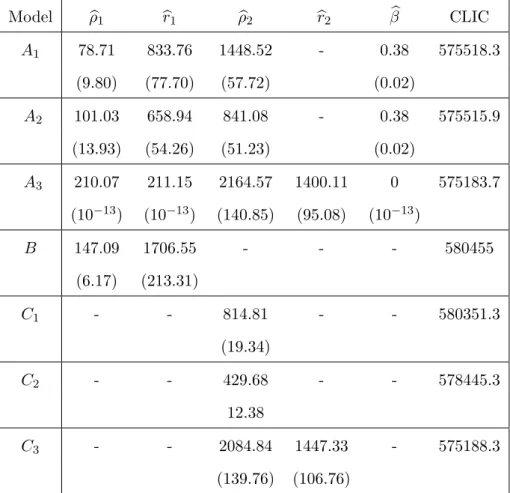
According to the CLIC value (Table 3) , the preferred model is theM MmodelA3. Nevertheless,
the results for this model, here reported for completeness, have to be carefully considered because
the estimate ofβ is virtually indistinguishable from zero, pointing out there is no mixture between
the max-stable process and the asymptotically independent one. For β = 0 the parameters of
the max-stable component are not identifiable and this fact affects the values of the estimates,
their standard errors and finally the CLIC value. Moreover model A3 reduces to model C3 for
β = 0 which corresponds the second best CLIC value, indicating some evidence for asymptotic
independence for all distances.
Setting aside A3 we reconsider the empirical and fitted values for ˆχ(h, u) and ˆχ¯(h, u), u= 0.9
and u= 0.95, for the three best models in each class, namelyA2,B andC3 (see Figure 9). Model
B seems to overestimate the asymptotic dependence at large distances. Again the fits of A2 and
C3 look overall similar with a slight preference for A2.
Finally, in order to illustrate the behavior of the models and check the fitting, we consider empirical and simulation based model estimates of few conditional probabilities. We choose the
sites1in the top-right corner of the map (see Figure 3) as a reference location and we consider three
subsets of sitesS1 ={s2, s3, s6, s8, s10},S2 ={s11, s13, s14, s15, s18} andS3 ={s25, s26, s27, s28, s29}
that roughly correspond to three different classes of distances from s1. Then we compute the
conditional probabilities Pr(Z(s) > z, s ∈ Si | Z(s1) > z), i = 1,2,3 for different large values
of p such that Pr(Z(s1) ≤ z) = p. The confidence intervals in Figure 10 are based on block
bootstrapping of simulated daily data. The overall impression is that the max-stable model B is
not able to describe the extremal dependence at medium (S2) and large distances (S3). Model
C3 basically overestimates the empirical probabilities for different thresholds and exhibits a lack of
fitting for relative small distances (S1). On the other hand the fitting of modelA2 is more consistent
at different thresholds and distances. Lastly note that both models agree for very large thresholds. These findings indicate that the max-mixture models we propose add modeling flexibility to spatial extreme analysis and seem able to encompass different degrees of spatial extremal dependence.
Model ρb1 br1 ρb2 br2 βb CLIC A1 78.71 833.76 1448.52 - 0.38 575518.3 (9.80) (77.70) (57.72) (0.02) A2 101.03 658.94 841.08 - 0.38 575515.9 (13.93) (54.26) (51.23) (0.02) A3 210.07 211.15 2164.57 1400.11 0 575183.7 (10−13) (10−13) (140.85) (95.08) (10−13) B 147.09 1706.55 - - - 580455 (6.17) (213.31) C1 - - 814.81 - - 580351.3 (19.34) C2 - - 429.68 - - 578445.3 12.38 C3 - - 2084.84 1447.33 - 575188.3 (139.76) (106.76)
Table 3: Summary of the fitted models based on the daily exceedances from the Australian data. Standard errors are reported in parentheses.
6. CONCLUSION
In this paper we have proposed an unifying spatial model which combines different degrees of ex-tremal dependence depending on the distance between pairs of sites. Our approach exploits the max-mixture model proposed by Wadsworth and Tawn (2012) and focuses on the possible detec-tion of pairwise max-stable dependence at short distances, asymptotic independence at intermediate ones and possibly exact independence at large distances. At short distances the extremal depen-dence is driven by a truncated extremal Gaussian max-stable process (Schlather, 2002) whereas at larger distances asymptotic independence is induced by any stochastic process with bivariate distributions satisfying a general condition proposed by Ledford and Tawn (1996). In this respect the hybrid models in Wadsworth and Tawn (2012) are particular instances.
Due to the intractability of the multivariate likelihoods parametric inference is carried out using a composite likelihood approach. A small and preliminary simulation study has shown that the inference procedure performs well, even when we have considered the boundary values for the
mixture parameter.
In our real example we have highlighted that the max-mixture approach appears of interest for modeling environmental data. In particular it has the merit to overcome the limits of the max-stable models in which only asymptotic dependence or exact independence can be modeled.
Our attention has been concentrated on modeling the spatial dependence. In the future, we plan to consider spatio-temporal extensions that have fundamental interest in practice. Currently space-time models are still taking up little space in the literature and the major emphasis is in modeling asymptotic dependence treating the time just as additional dimension of the space (Davis et al., 2013; Huser and Davison, 2014). However it seems reasonable to suppose that the spatial and temporal components behave asymptotically in a different way.
ACKNOWLEDGEMENTS
The research was partially supported by ANR-McSim and GICC-Miraccle projects and by the Labex NUMEV. 137478, 2004. We are also indebted with Simone Padoan and the referees for comments that have led to improvements in the article.
REFERENCES
Ancona-Navarrete, M., and Tawn, J. (2002), “Diagnostics for pairwise extremal dependence in
spatial processes,” Extremes, 5, 271–285.
Bacro, J. N., and Gaetan, C. (2012), “A review on spatial extreme modelling,” in Advances and
Challenges in Space-Time Modelling of Natural Events, eds. E. Porcu, J. M. Montero, and M. Schlather, New York: Springer, pp. 103–124.
Bacro, J. N., and Gaetan, C. (2014), “Estimation of spatial max-stable models using threshold
exceedances,” Statistics and Computing, 24, 651–662.
Beirlant, J., Goegebeur, Y., Segers, J., and Teugels, J. (2004), Statistics of Extremes: Theory and
Applications, New York: John Wiley & Sons.
Bingham, N. H., Goldie, C. M., and Teugels, J. L. (1987),Regular variation, Vol. 27 ofEncyclopedia
of Mathematics and its Applications, Cambridge: Cambridge University Press.
Carlstein, A. (1986), “The use of subseries values for estimating the variance of a general statistic
from a stationary sequence,” The Annals of Statistics, 14, 1171–1179.
Casson, E., and Coles, S. G. (1999), “Spatial regression models for extremes,”Extremes, 1, 449–468.
Coles, S., Heffernan, J., and Tawn, J. (1999), “Dependence measures for extremes value analyses,”
Extremes, 2, 339–365.
Cooley, D., Nychka, D., and Naveau, P. (2007), “Bayesian spatial modeling of extreme precipitation
return levels,” Journal of the American Statistical Association, 102, 824–840.
Davis, R. A., Kl¨uppelberg, C., and Steinkohl, C. (2013), “Max-stable processes for modeling
ex-tremes observed in space and time,” Journal of the Korean Statistical Society, 42, 399–414.
Davison, A. C., and Gholamrezaee, M. M. (2012), “Geostatistics of extremes,” Proceedings of the
Royal Society London, Series A, 468, 581–608.
Davison, A. C., Huser, R., and Thibaud, A. (2013), “Geostatistics of dependent and asymptotically
independent extremes,” Mathematical Geosciences, 45, 511–529.
Davison, A. C., Padoan, S. A., and Ribatet, M. (2012), “Statistical modelling of spatial extremes,”
de Haan, L. (1984), “A spectral representation for max-stable processes,” Annals of Probability, 12, 1194–1204.
de Oliveira, T. (1962), “Structure theory of bivariate extremes: extensions,” Estudos de
Mathem`atica, Estatistica e Econometrica, 7, 165–195.
Engelke, S., Malinowski, A., Kabluchko, Z., and Schlather, M. (2015), “Estimation of H¨usler-Reiss
distributions and Brown-Resnick processes,” Journal of the Royal Statistical Society: Series B,
77, 239–265.
Fawcett, L., and Walshaw, D. (2007), “Improved estimation for temporally clustered extremes,”
Environmetrics, 18, 173–188.
Ferreira, A., and de Haan, L. (2014), “The generalized Pareto process; with a view towards
appli-cation and simulation,” Bernoulli, 20, 1717–1737.
Gaetan, C., and Grigoletto, M. (2007), “A hierarchical model for the analysis of spatial rainfall
extremes,” Journal of Agricultural Biological and Environmental Statistics, 12, 434–449.
Guyon, X. (1995),Random Fields on a Network, New York: Springer.
Huser, R., and Davison, A. C. (2014), “Space-time modeling of extreme events,” Journal of the
Royal Statistical Society, Series B, 76, 439–461.
Jeon, S., and Smith, R. (2012), Dependence structure of spatial extremes using threshold approach,, Technical report, arXiv:1209.6344.
Kabluchko, Z., Schlather, M., and de Haan, L. (2009), “Stationary max-stable fields associated to
negative definite functions,”The Annals of Probability, 37, 2042–2065.
Lavery, B., Kariko, A., and Nicholls, N. (1992), “A historical rainfall data set for Australia,”
Australian Meteorology Magazine, 40, 33–39.
Ledford, A., and Tawn, J. (1997), “Modelling dependence within joint tail regions,”Journal of the
Royal Statistical Society, Series B, 59, 475–499.
Ledford, A., and Tawn, J. (1998), “Concomitant tail behaviour for extremes,”Advances in Applied
Ledford, A. W., and Tawn, J. A. (1996), “Statistics for near independence in multivariate extreme
values,” Biometrika, 83, 169 –187.
Lindsay, B. (1988), “Composite likelihood methods,”Contemporary Mathematics, 80, 221–239.
Mardia, K. V., and Watkins, A. J. (1989), “On multimodality of the likelihood in the spatial linear
model,” Biometrika, 76, 289–295.
Opitz, T. (2013), “Extremal t processes: elliptical domain of attraction and a spectral
representa-tion,” Journal of Multivariate Analysis, 122, 409–413.
Padoan, S. A. (2013), “Extreme dependence model based on event magnitude,”Journal of
Multi-variate Analysis, 122, 1–19.
Padoan, S. A., Ribatet, M., and Sisson, S. (2010), “Likelihood-based inference for max-stable
processes,” Journal of the American Statistical Association, 105, 263–277.
Resnick, S. (1987),Extreme values, Regular variation and Point Processes, New York: Springer.
Ribatet, M., Cooley, D., and Davison, A. (2012), “Bayesian inference for composite likelihood
models and an application to spatial extremes,” Statistica Sinica, 22, 813–845.
Sang, H., and Gelfand, A. (2010), “Continuous spatial process models for spatial extreme values,”
Journal of Agricultural, Biological, and Environmental Statistics, 15, 49–65.
Schlather, M. (2002), “Models for stationary max-stable random fields,” Extremes, 5, 33–44.
Schlather, M., and Tawn, J. A. (2003), “A dependence measure for multivariate and spatial extreme
values: properties and inference,” Biometrika, 90, 139–156.
Serinaldi, F., B´ardossy, A., and Kilsby, C. G. (2014), “Upper tail dependence in rainfall extremes:
would we know it if we saw it ?,” Stochastic Environmental Research and Risk Assessment,
29, 1211–1233.
Sibuya, M. (1960), “Bivariate extreme statistics,”Annals of the Institute of Statistical Mathematics,
11, 195–210.
Smith, R. L. (1990), “Max-stable processes and spatial extremes,”, Preprint. University of Surrey. Thibaud, E., Mutzner, R., and Davison, A. C. (2013), “Threshold modeling of extreme spatial
Varin, C. (2008), “On composite marginal likelihoods,” Advances in Statistical Analysis, 92, 1–28. Varin, C., and Vidoni, P. (2005), “A note on composite likelihood inference and model selection,”
Biometrika, 92, 519–528.
Wadsworth, J., and Tawn, J. (2012), “Dependence modelling for spatial extremes,” Biometrika,
99, 253–272.
Wadsworth, J., and Tawn, J. (2014), “Efficient inference for spatial extreme value processes
β =1 β =0.75 β =0.5 β =0.25 β =0 −2.3 −1.7 −1.11 −0.510.09 0.69 1.29 1.89 2.49 3.09 3.69 4.29 4.89 5.49
Figure 1: Simulations of the M Mβ model (10) on the logarithm scale according different values
of β ∈ {0,0.25,0.50,0.75,1}. The compact set B is taken as a disc with a fixed radius r = 0.25.
An exponential correlation function with parameterρ1 = 0.2 is chosen for the underlying Gaussian
process. For the AI process a Gaussian random field is considered with a spherical correlation
0.0 0.2 0.4 0.6 0.8 1.0 ρ1 ρ2 β r 0.0 0.2 0.4 0.6 0.8 1.0 ρ1 ρ2 β r 0.0 0.2 0.4 0.6 0.8 1.0 ρ1 ρ2 β r 0.0 0.2 0.4 0.6 0.8 1.0 ρ1 ρ2 β r
Figure 2: Boxplots of 500 estimates from 1000 independent copies of theM Mβ model (from left to
right: β = 0, β = 0.25, β = 0.75 and β = 1) withρ1 = 0.2, ρ2 = 0.8 and r = 0.25. For β = 0 and
β = 1, only the results for the identifiable parameters are reported.
1 5 6 8 9 10 11 13 14 15 17 18 19 28 29 31 2 3 4 7 12 16 20 21 22 23 24 25 26 27 30
Figure 3: Geographical locations of the 31 meteorological stations in the East Australia. Stations with a label in bold character are used for model inference and the other stations are put aside for validating the models
● ● ● ● ● ● ● ● ● ● ● ● ● ● ● ● ● ● ● ● ● ●● ● ● ● ● ●● ● ●● ● ● ● ● ● ● ● ● ● ● ● ● ● ● ● ● ● ● ● ●● ●● ● ● ● ● ● ● ● ● ● ● ● ● ● ● ● ● ● ● ● ● ● ● ● ● ● ● ● ● ●● ● ● ● ●● ● ● ● ● ● ● ● ● ● ● ● ● ● ● ● ● ● ● ● ● ●● ●● ● ● ● ● ● ● ● ● ● ● ●● ● ● ● ● ● ● ● ● ● ● ● ● ●● ● ● ● ● ● ●● ● ● ● ● ● ● ● ● ● ● ● ● ● ● ● ● ● ● ● ● ●● ● ● ● ●● ● ● ● ● ● ● ● ● ● ● ● ● ● ● ● ● ● ● ●●● ● ● ● ● ● ● ● ● ● ● ● ● ● ● ● ● ● ● ● ● ● ●● ● ● ● ● ● ● ● ● ● ● ● ● ● ● ● ● ● ● ● ● ● ● ● ●● ● ● ● ● ● ● ● ● ● ● ● ● ● ● ● ● ● ● ● ● ● ●● ● ● ● ● ●● ● ●● ● ● ● ● ● ● ● ● ● ● ●● ● ● ● ● ● ● ● ● ● ● ● ● ● ● ● ● ● ● ● ● ● ● ● ● ● ● ●● ● ● ● ● ● ● ● ● ● ● ● ● ● ● ● ● ● ● ● ● ● ● ● ● ● ● ● ● ● ● ● ● ● ● ● ● ● ● ● ● ● ● ● ● ● ● ● ● ● ● ● ● ● ● ● ● ● ● ● ● ● ● ● ● ● ● ● ● ● ● ● ● ● ● ● ● ● ● ● ● ● ● ● ● ● ● ● ● ● ● ● ● ● ● ● ● ● ● ● ● ● ● ● ● ● ● ● ● ● ● ● ● ● ● ● ● ● ● ● ● ● ● ● ● ● ● ● ● ● ● ●● ● ● ● ● ● ● ● ● ● ● ● ● ● ● ● ● ● ● ● ● ● ●● ● ● ● ● ● ● ● ● ●● ● ● ● ● ● ● ● ● ● ● ● ● ● ● ● ● ● ● ● ● ● ● ● ● ● ● ● ● ● ● ● ● ● ● ● ● ● ● ● ● ● ● ● ● ● ● ● ● 0 500 1000 1500 0.0 0.1 0.2 0.3 0.4 0.5 0.6 0.7 distance χ 0 π4 π2 3π4 ● ● ● ● ● ● ● ● ● ● ● ● ● ● ● ● ● ● ● ● ● ● ●● ● ● ● ● ● ● ● ● ● ● ● ● ● ● ● ● ● ● ● ● ● ● ● ● ● ● ● ●● ●● ● ● ● ● ● ● ● ● ● ● ● ● ● ● ● ● ● ● ● ● ● ● ● ● ● ● ● ● ● ● ● ● ● ● ● ● ● ● ● ● ● ● ● ● ● ● ● ● ● ● ● ● ● ● ● ●● ●● ● ● ● ● ● ● ● ● ● ● ●● ● ● ● ● ● ● ● ● ● ● ● ● ●● ● ● ● ● ● ●● ● ● ● ● ● ● ● ● ● ● ● ● ● ● ● ● ● ● ● ● ● ● ● ● ● ● ● ● ● ● ● ● ● ● ● ● ● ● ● ● ● ● ● ● ● ●●● ● ● ● ● ● ● ● ● ● ● ● ● ● ● ● ● ● ● ● ● ● ●● ● ● ● ● ● ● ● ● ● ● ● ● ● ● ● ● ● ● ● ● ● ● ● ●● ● ● ● ● ● ● ● ● ● ● ● ● ● ● ● ● ● ● ● ● ● ●● ● ● ● ● ● ● ● ● ● ● ● ● ● ● ● ● ● ● ● ●● ● ● ● ● ● ● ● ● ● ● ● ● ● ● ● ● ● ● ● ● ● ● ● ● ● ● ●● ● ● ● ● ● ● ● ● ● ● ● ● ● ● ● ● ● ● ● ● ● ● ● ● ● ● ● ● ● ● ● ● ● ● ● ● ● ● ● ● ● ● ● ● ● ● ● ● ● ● ● ● ● ● ● ● ● ● ● ● ● ● ● ● ● ● ● ● ● ● ● ● ● ● ● ● ● ● ● ● ● ● ● ● ● ● ● ● ● ● ● ● ● ● ● ● ● ● ● ● ● ● ● ● ● ● ● ● ● ● ● ● ● ● ● ● ● ● ● ● ● ● ● ● ● ● ● ● ● ● ●● ● ● ● ● ● ● ● ● ● ● ● ● ● ● ● ● ● ● ● ● ● ●● ● ● ● ● ● ● ● ● ●● ● ● ● ● ● ● ● ● ● ● ● ● ● ● ● ● ● ● ● ● ● ● ● ● ● ● ● ● ● ● ● ● ● ● ● ● ● ● ● ● ● ● ●● ● ● ● ● 0 500 1000 1500 0.0 0.2 0.4 0.6 0.8 distance χ 0 π4 π2 3π4
Figure 4: Empirical evaluation of the functionsχb(h, u) (left) andχb¯(h, u) (right) atu= 0.975. Gray circles give empirical value between all available pairs. Lines represent smoothed values of the
empirical estimates using the pairs in the directional sectors (−π/8,π/8], (π/8, 3π/8], (3π/8, 5π/8]
and (5π/8, 7π/8]. 0 500 1000 1500 0.0 0.1 0.2 0.3 0.4 0.5 0.6 0.7 distance χ 0.9 0.95 0.975 0.99 0.995 0 500 1000 1500 0.0 0.2 0.4 0.6 0.8 distance χ 0.9 0.95 0.975 0.99 0.995
Figure 5: Smoothed values of the empirical estimates of the functions ˆχ(h, u) (left) and ˆχ¯(h, u)
0 500 1000 1500 0.0 0.2 0.4 0.6 0.8 1.0 q0.9 Distance χ A1 B C2 ● ● ● ● ● ● ●● ● ● ● ● ● ● ● ● ● ● ● ●● ● ● ● ● ● ● ● ● ● ● ●● ● ● ● ● ● ● ● ● ● ●● ● ● ● ● ● ● ● ● ● ● ●● ● ●● ● ● ● ● ● ● ● ● ● ● ● ● ● ● ● ● ● ● ● ●● ● ● ● ● ●●● ● ● ● ● ● ● ● ● ● ● ● ● ● ● ● ● ● ● 0 500 1000 1500 0.0 0.2 0.4 0.6 0.8 1.0 q0.9 Distance χ ● ● ● ● ● ● ● ● ● ● ● ●● ● ● ● ● ● ● ● ● ● ● ●●●●●● ● ● ● ● ● ● ● ● ● ● ● ●●● ● ● ● ● ● ● ● A1 B C2 0 500 1000 1500 0.0 0.2 0.4 0.6 0.8 1.0 q0.95 Distance χ A1 B C2 ● ● ● ● ● ● ●● ● ● ● ● ● ● ● ● ● ● ● ●● ● ● ● ● ● ● ● ● ● ● ●● ● ● ● ● ● ● ● ● ● ●● ● ● ● ● ● ● ● ● ● ● ●● ● ●● ● ● ● ● ● ● ● ● ● ● ● ● ● ●● ● ● ● ● ●● ● ● ● ● ● ● ● ● ● ● ● ● ● ● ● ● ● ● ● ● ● ● ● ● ● 0 500 1000 1500 0.0 0.2 0.4 0.6 0.8 1.0 q0.95 Distance χ ● ● ● ● ● ●●●●●●● ● ●● ●● ● ● ●● A1 B C2
Figure 6: Site-wise winter maxima: empirical and fitted values for ˆχ(h, u) and ˆχ¯(h, u). Empirical
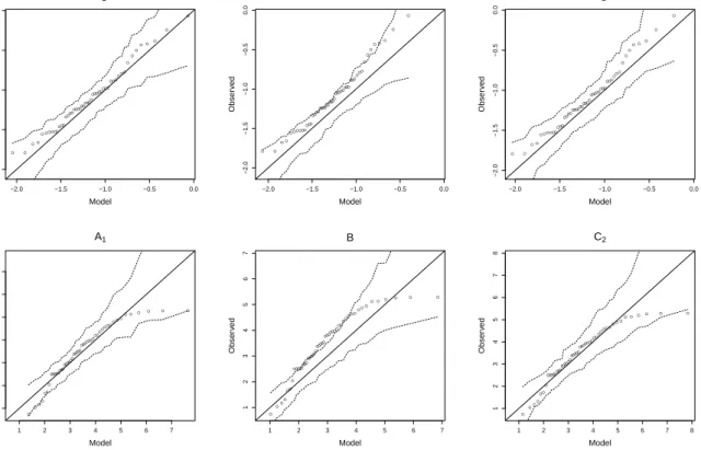
● ●● ● ●● ● ● ●●● ●●● ●●●●●●●●●●●● ●●●●●● ●● ●●● ● ●● ● ● ● ● ●● ● ● ● −2.0 −1.5 −1.0 −0.5 0.0 −2.0 −1.5 −1.0 −0.5 0.0 A1 Model Obser v ed ● ●● ● ●● ● ●● ●● ●●● ●●●●●●●● ●●●●● ●●●●● ●● ● ●●● ●● ● ● ● ● ●● ● ● ● −2.0 −1.5 −1.0 −0.5 0.0 −2.0 −1.5 −1.0 −0.5 0.0 B Model Obser v ed ● ●● ● ●● ● ●● ●● ●●● ●●●●●● ●● ●●● ●●●●●●● ●● ●●● ● ●● ● ● ● ● ● ● ● ● ● −2.0 −1.5 −1.0 −0.5 0.0 −2.0 −1.5 −1.0 −0.5 0.0 C2 Model Obser v ed ● ●●● ●●● ● ●●● ●● ●●●●●●●●● ●●●● ●●●●● ●●●●●● ● ●● ● ●● ● ●● ● ● ● 1 2 3 4 5 6 7 1 2 3 4 5 6 7 A1 Model Obser v ed ● ●● ● ●● ● ● ●●● ● ● ●●●●●●●●● ●●● ● ●●●●●●●●● ●● ● ●● ● ●● ●●● ● ● ● 1 2 3 4 5 6 1 2 3 4 5 6 B Model Obser v ed ● ●● ● ●● ● ●●● ● ●● ●●●●●●●●● ●●●● ●●●●●●●●●●● ●●● ● ●● ● ●● ● ● ● 1 2 3 4 5 6 7 1 2 3 4 5 6 7 C2 Model Obser v ed
Figure 7: Site-wise winter maxima: quantile-quantile plots for the minimum and maximum values
on the validation data set (15 sites). The three columns correspond to fitted models models A1,
B and C2, respectively. The top row compares the minimum of the validation data set with its
corresponding value under the fitted models. The bottom row compares in the same way the maximum values on the validation data set.
● ● ● ● ● ●● ●●● ●●● ●●●● ●●●●●● ●●●● ●●●●● ●●● ●●● ●●● ● ● ● ●●● ● ● −2.0 −1.5 −1.0 −0.5 0.0 −2.0 −1.5 −1.0 −0.5 0.0 A1 Model Obser v ed ● ● ● ● ● ●●●●● ●●● ●●●● ●●●●●● ●●●● ●●●●● ●●● ●●● ●●● ● ● ● ● ● ● ● ● −2.0 −1.5 −1.0 −0.5 0.0 −2.0 −1.5 −1.0 −0.5 0.0 B Model Obser v ed ● ● ● ● ● ●● ●●● ●●● ●● ●●●●●● ●●●●● ● ●●●●● ●●● ●●● ●● ● ● ● ● ● ●● ● ● −2.0 −1.5 −1.0 −0.5 0.0 −2.0 −1.5 −1.0 −0.5 0.0 C2 Model Obser v ed ● ●●● ●● ● ●●●●●●●● ●●●●●● ●●●●● ●●●●●●●●● ●●●●●● ● ● ● ●● ● ● ● 1 2 3 4 5 6 7 1 2 3 4 5 6 7 A1 Model Obser v ed ● ● ●● ●● ● ●●●●● ●●● ●●●● ●● ●●●●● ●●●●●●● ●● ●● ● ●● ●●● ●●● ● ● ● 1 2 3 4 5 6 7 1 2 3 4 5 6 7 B Model Obser v ed ● ●● ● ●● ● ●●●●●●●● ●●●●●● ●●●●● ●●●●●● ●●● ●●●●●● ● ● ● ●● ● ● ● 1 2 3 4 5 6 7 8 1 2 3 4 5 6 7 8 C2 Model Obser v ed
Figure 8: Site-wise winter maxima: quantile-quantile plots for the minimum and maximum values
on the complete data set (31 sites). The three columns correspond to fitted models models A1,
B and C2, respectively. The top row compares the minimum of the validation data set with its
corresponding value under the fitted models. The bottom row compares in the same way the maximum values on the validation data set
0 500 1000 1500 0.0 0.2 0.4 0.6 0.8 1.0 q0.9 Distance χ A2 B C3 ● ● ● ● ● ● ●●● ● ● ● ● ● ● ● ● ● ● ●● ● ● ● ● ● ● ● ● ● ● ●●● ● ● ● ● ● ● ● ● ● ● ● ● ● ● ● ● ● ● ● ● ● ● ● ● ● ● ● ● ● ● ● ● ● ● ● ● ● ●● ● ● ● ● ● ● ● ● ● ● ● ● ● ● ● ● ● ● ● ● ● ● ● ● ● ● ● ● ● ● ● ● 0 500 1000 1500 0.0 0.2 0.4 0.6 0.8 1.0 q0.9 Distance χ ● ● ● ● ● ● ● ● ● ● ● ● ● ● ● ● ● ● ● ● ● ● ● ● ● ● ● ● ● ● ● ●●● ● ● ● ● ● ● ● ● ● ● ● ● ● ● ● ● ● ● ● ● ●● ● ● ● ● ● ● ● ● ● ● ● ● ● ● ● ● ● ● ● ● ● ● ● ● ● ● ● ● ● ● ● ● ● ● ● ● ● ● ● ● ● ● ● ● ● ● ● ● ● A2 B C3 0 500 1000 1500 0.0 0.2 0.4 0.6 0.8 1.0 q0.95 Distance χ A2 B C3 ● ● ● ● ● ● ●●● ● ● ● ● ● ● ● ● ● ● ●● ● ● ● ● ● ● ● ● ● ● ● ● ● ● ● ● ● ● ● ● ● ● ● ● ● ● ● ● ● ● ● ● ● ● ● ● ● ● ● ● ● ● ● ● ● ● ● ● ●● ● ● ● ● ● ● ● ● ● ● ● ● ● ● ● ● ● ● ● ● ● ● ● ● ● ● ● ● ● ● ● ● ● ● 0 500 1000 1500 0.0 0.2 0.4 0.6 0.8 1.0 q0.95 Distance χ ● ● ● ● ● ● ●● ● ● ● ● ● ● ● ● ● ● ● ●● ● ● ● ● ● ● ● ● ● ● ● ●● ● ● ● ● ● ● ● ● ● ● ● ● ● ● ● ● ● ● ● ● ● ● ● ● ● ● ● ● ● ● ● ● ● ● ● ●● ● ● ● ● ● ● ● ● ● ● ● ● ● ● ● ● ● ● ● ● ● ● ● ● ● ● ● ● ● ● ● ● ● ● A2 B C3
Figure 9: Winter daily data: empirical and fitted values for ˆχ(h, u) and ˆχ¯(h, u). Empirical values
are computed using the validation data set and models are fitted using theququantile exceedances.
2.0 2.5 3.0 3.5 4.0 4.5 5.0 5.5 0.00 0.05 0.10 0.15 0.20 0.25 A2 −log(1−p)
Cond. Exc. Prob
. ● ● ● ● ● ● ● ● 2.0 2.5 3.0 3.5 4.0 4.5 5.0 5.5 0.00 0.05 0.10 0.15 0.20 0.25 B −log(1−p)
Cond. Exc. Prob
. ● ● ● ● ● ● ● ● 2.0 2.5 3.0 3.5 4.0 4.5 5.0 5.5 0.00 0.05 0.10 0.15 0.20 0.25 C3 −log(1−p)
Cond. Exc. Prob
. ● ● ● ● ● ● ● ● 2.0 2.5 3.0 3.5 4.0 4.5 5.0 5.5 0.00 0.05 0.10 0.15 A2 −log(1−p)
Cond. Exc. Prob
. ● ● ● ● ● ● ● ● 2.0 2.5 3.0 3.5 4.0 4.5 5.0 5.5 0.00 0.05 0.10 0.15 B −log(1−p)
Cond. Exc. Prob
. ● ● ● ● ● ● ● ● 2.0 2.5 3.0 3.5 4.0 4.5 5.0 5.5 0.00 0.05 0.10 0.15 C3 −log(1−p)
Cond. Exc. Prob
. ● ● ● ● ● ● ● ● 2.0 2.5 3.0 3.5 4.0 4.5 5.0 5.5 0.00 0.02 0.04 0.06 0.08 0.10 0.12 A2 −log(1−p)
Cond. Exc. Prob
. ● ● ● ● ● ● ● ● 2.0 2.5 3.0 3.5 4.0 4.5 5.0 5.5 0.00 0.02 0.04 0.06 0.08 0.10 0.12 B −log(1−p)
Cond. Exc. Prob
. ● ● ● ● ● ● ● ● 2.0 2.5 3.0 3.5 4.0 4.5 5.0 5.5 0.00 0.02 0.04 0.06 0.08 0.10 0.12 C3 −log(1−p)
Cond. Exc. Prob
. ● ● ● ● ● ● ● ●
Figure 10: Winter daily data: empirical and fitted values for the conditional probabilities Pr(Z(s)>
z, s ∈ S |Z(s1) > z). The three columns correspond to modelsA2, B and C3, respectively. Top
row: S = {s2, s3, s6, s8, s10} (near sites data set); middle row S ={s11, s13, s14, s15, s18} (medium
sites data set); bottom row: S = {s25, s26, s27, s28, s29} (far sites data set). The 1−p values are