Motion Segmentation for Autonomous Robots Using 3D Point Cloud Data

(1)

Worcester Polytechnic Institute Worcester Polytechnic Institute

Digital WPI

Masters Theses (All Theses, All Years) Electronic Theses and Dissertations 2020-05-13

Motion Segmentation for Autonomous Robots Using 3D Point

Cloud Data

Amey S. Kulkarni

Worcester Polytechnic Institute

Follow this and additional works at: https://digitalcommons.wpi.edu/etd-theses

Repository Citation Repository Citation

Kulkarni, Amey S., "Motion Segmentation for Autonomous Robots Using 3D Point Cloud Data" (2020). Masters Theses (All Theses, All Years). 1370.

https://digitalcommons.wpi.edu/etd-theses/1370

(2)

Motion Segmentation for Autonomous Robots Using 3D

Point Cloud Data

by

Amey Sunil Kulkarni

A Thesis

Submitted to the Faculty of the

WORCESTER POLYTECHNIC INSTITUTE In partial fulfillment of the requirements for the

Degree of Master of Science in

Robotics Engineering

May 2020

APPROVED:

Professor Xinming Huang, Thesis Advisor

Professor Ziming Zhang, Committee Member

(3)

Abstract

Achieving robot autonomy is an extremely challenging task and it starts with de-veloping algorithms that help the robot understand how humans perceive the en-vironment around them. Once the robot understands how to make sense of its environment, it is easy to make efficient decisions about safe movement. It is hard for robots to perform tasks that come naturally to humans like understanding sign-boards, classifying traffic lights, planning path around dynamic obstacles, etc. In this work, we take up one such challenge of motion segmentation using Light De-tection and Ranging (LiDAR) point clouds. Motion segmentation is the task of classifying a point as either moving or static. As the ego-vehicle moves along the road, it needs to detect moving cars with very high certainty as they are the areas of interest which provide cues to the ego-vehicle to plan it’s motion. Motion segmen-tation algorithms segregate moving cars from static cars to give more importance to dynamic obstacles.

In contrast to the usual LiDAR scan representations like range images and regu-lar grid, this work uses a modern representation of LiDAR scans using permutohedral lattices. This representation gives ease of representing unstructured LiDAR points in an efficient lattice structure. We propose a machine learning approach to per-form motion segmentation. The network architecture takes in two sequential point clouds and performs convolutions on them to estimate if 3D points from the first point cloud are moving or static. Using two temporal point clouds help the network in learning what features constitute motion. We have trained and tested our learn-ing algorithm on the Flylearn-ingThlearn-ings3D dataset and a modified KITTI dataset with simulated motion.

(4)

Acknowledgements

A smooth sea never made a skilled sailor

-Franklin D. Roosevelt

I consider this thesis to be a very important achievement in my life and I am immensely grateful to a lot of people without whom this wouldn’t have been possi-ble. I would like to express my gratitude to my advisor Prof.Xinming Huang who gave me an opportunity to pursue research in the field of my interest. His uncon-ditional support helped me explore a variety of approaches to the problem. His willingness to help and brainstorming sessions with him provided immense help. I am also grateful to Prof.Ziming Zhang whose expertise has helped me a great deal in achieving the results in this thesis. His prompt responses, constructive criticism, and brilliant ideas helped me develop research skills and improve my knowledge in the field of perception and machine learning. I am also extremely thankful to Prof.Riad Hammoud who introduced me to the field of SLAM and encouraged me to pursue research.

I would also like to thank my lab mates Yiming, Mahdi, Yecheng and Lin who helped me in brainstorming ideas and with solving technical glitches. I am extremely grateful to my roommates Tyagaraja, Akshay, and Denim who were always there for me during my MS. Apart from their help in technical matters, their amicable nature and the discussions we had offered me some respite. I also thank all my peers from WPI who always inspired me to work harder.

Most importantly, I am extremely grateful to my parents for supporting me in all my endeavours unconditionally. I had given up on this thesis, but their assurance and their motivation is what kept me going. I thank them for all the sacrifices they

(5)

List of Figures

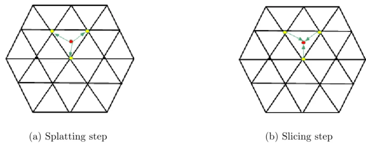
1.1 A LiDAR scan taken from WPI neighborhood [27] . . . 5 3.1 Major processes for motion segmentation and system flow . . . 23 3.2 A 2-dimensional permutohedral lattice [1] . . . 26 3.3 In (a), the red input point interpolates to the yellow vertices of the

enclosing simplex and in (b), interpolations are performed to get back the original input point . . . 28 3.4 Splat-Conv-Slice steps for BCL layers using a permutohedral lattice [15] 29 3.5 Barycentric interpolation . . . 30 3.6 Network architecture for motion segmentation. The values in brackets

are the number of output channels of the layers. Two values in the CorrBCL layers correspond to Patch correlation and Displacement filtering. . . 33 3.7 Log loss graph when the ground truth is 1 . . . 35 3.8 Focal loss for different values of γ when the ground truth is 1 . . . 37 3.9 Demonstration of different motion content in point cloud samples.

The red points indicate motion and the green points indicate static points . . . 43

(8)

List of Tables

4.1 Comparison of mean evaluation metrics based on different loss func-tions: FlyingThings3D dataset . . . 47 4.2 Mean precision and mean recall values for different losses:

FlyingTh-ings3D dataset . . . 48 4.3 Inference time for different sizes of point clouds: FlyingThings3D

dataset . . . 48 4.4 Comparison with prior methods: FlyingThings3D dataset . . . 49 4.5 Evaluating model trained on FlyingThings3D with BCE loss function

on the modified KITTI dataset. All values are mean values. . . 51 4.6 Mean precision and mean recall values for the task of using BCE

model trained on FlyingThings3D for inference on the modified KITTI dataset. . . 51 4.7 Comparison of evaluation metrics based of loss function for modified

KITTI dataset . . . 53 4.8 Mean precision and mean recall values for different losses: modified

KITTI dataset . . . 53 4.9 Mean and standard deviation of F1 scores for moving points with

(9)

4.10 Inference time for different sizes of point clouds : modified KITTI dataset . . . 55

(10)

Chapter 1 Introduction

Robots have become an important part of today’s industry and economy. Robots are being developed for a variety of applications like industrial robotics, autonomous vehicles, indoor and outdoor security, cleaning, medical surgeries, exoskeletons, de-fense, etc. A certain level of autonomy is advantageous in all kinds of robots. Autonomy reduces the dependence of robots on humans for decision making. All robots in lesser or higher proportions follow a sense-plan-act methodology. The robots sense their environment with different kinds of sensors. Using the observa-tions from the environment as prior, robots plan their future using a collection of algorithms. These plans are brought to life using actuators like motors. If thesense phase is not executed with high accuracy, all the decisions the robots take will be flawed and the robot will be rendered unsafe for use. To explain with an example, if an autonomous vehicle fails tosense a pedestrian standing in front of it, then the trajectory that it will plan will be through the pedestrian. The action of following this trajectory will result in an unfortunate accident.

This work focuses on improving thesense phase for a representative application of autonomous vehicles. The application of the motion segmentation algorithm

(11)

pro-posed in this work is not constrained to autonomous vehicles and can be translated to indoor, aerial, and humanoid robots with minor changes. Autonomous vehicles are an exciting application in robotics and currently, it is a multi-billion dollar indus-try that is expected to grow exponentially in the coming years. Autonomous vehicles usually use a sensor suite consisting of, but not limited to cameras, LiDARs(Light Detection and Ranging), GPS(Global Positioning System), RADARs(Radio Detec-tion and Ranging), IMUs(Inertial Measurement Unit), and encoders. New sensors are coming into existence at a fast pace. The event camera is one such new promis-ing sensor. These sensors help the system perceive the environment around the car. The major tasks which consist of understanding the environment are foreground-background detection, moving object segmentation and tracking, object trajectory forecasting, optical/scene flow estimation, etc. These tasks indirectly help in devel-oping robust planning algorithms for obstacle avoidance, motion planning, etc.

We focus on theMotion Segmentationpart where the objective is to classify every point of the LiDAR scan as moving/dynamic or non-moving/static. We use these binary terms throughout this thesis. There have been some geometric algorithms to solve this task in the past. However, since the advent of Artificial Intelligence, many innovative solutions for the motion segmentation task based on deep learning networks have come to light. Our method is also based on using convolutional neural networks for performing this task. We propose the use of an hourglass-shaped neural network which takes in two sequential point clouds and predicts point-wise binary classification labels for the first point cloud.

(12)

1.1 Motivation

The challenge of Motion Segmentation has been studied in depth for modalities like cameras and RGB-D sensors. A lot of research papers have been published trying to solve this challenge using the above sensors. The advantage of LiDAR over these sensors is that it provides very accurate depth values for discrete points in its 360◦ range. Also, LiDARs can be used during night or in low light areas without

any modification. Despite these advantages, the research in the field of motion segmentation using LiDAR points clouds is underexplored. This is perhaps because the LiDAR sensors do not provide a rich variety of information like colors, texture, etc. One has to find the correlation between the distance values of neighboring points to arrive at any conclusion. It is extremely imperative to solve this challenge and our method is one such effort in this direction. Solving this problem will introduce us to a plethora of new research opportunities. The major areas that will benefit from a solution to the motion segmentation problem are - building long term static maps, motion prediction, accurate localization, tracking performance improvement, obstacle avoidance, etc.

Another major motivation to solve this problem is to make autonomous robots safer. When the system has better knowledge about the movement of all the traffic participants in its scene, it will be better prepared to take critical decisions.

Hence we propose a machine learning architecture that takes in two sequential 3D point clouds and gives out moving/non-moving predictions for points in the first point cloud. We have been careful about keeping this method computationally economic.

(13)

1.2 Background

Before going deep into the method, it is essential to understand the intricacies of LiDAR sensor measurements and to give an intuition about how the motion segmentation problem can be solved using this data.

1.2.1 Understanding LiDAR Data

LiDAR sensors are increasingly becoming common in the area of autonomous robots. LiDARs are being used on self-driving cars, warehouse robots, aerial robots, security robots, and they are also expected to arrive in mobile devices soon. This widespread acceptance of this sensor has become possible due to the falling prices of this sensor hardware.

LiDAR is an active remote sensor i.e it uses the light energy generated by its sys-tem and provides measurements from the environment without actually coming in contact with it. The LiDAR emits laser pulses and measures the time-of-flight(ToF) of the pulse return. The distance of this particular point from the sensor is then found by using the relation between the speed of light and the ToF. LiDAR sen-sors come in a variety of configurations. LiDARs can record 2-dimensional or 3-dimensional data. The 2D sensors record all their points on a single plane. The 3D sensors come with multiple light emitters stacked in a single vertical line so that points across multiple planes can be measured. The most common configurations of the 3D sensor are 16-line, 32-line, 64-line, and 128-line. The typical horizontal field of view of the sensor is 360◦ and the vertical field of view ranges from 30◦ to

120◦. A conventional LiDAR used on most autonomous robots is a spinning sensor.

The spinning helps it to map the whole 360◦ environment. The angle of rotation

(14)

LiDAR models also return an intensity value along with the point coordinates. The intensity value indicates the strength of the received light pulse. The returning strength depends on the reflectivity of the material on which the light strikes. The intensity values measured by the sensor are relative and largely depend on the wave-length of the light used, incident angle, and the material on which the light strikes. The intensity values are being used in object classification and aerial observation. Every point detected by the LiDAR can be represented as

~

p= (x, y, z, i)

wherex,y, z are the Cartesian coordinates in the sensor frame of reference and i is the intensity value. An image of a LiDAR scan taken from the neighborhoods of Worcester Polytechnic Institute is shown in Figure.1.1

The typical wavelengths of the light emitted from commonly available LiDAR sensors are 905nm and 1550nm. These wavelengths are chosen as they are in the invisible range and are relatively safe to human eyes.

(15)

1.2.2 Understanding Motion Segmentation

The task of motion segmentation is simply to distinguish moving points from non-moving points. Moving points belong to objects which are non-moving in the environ-ment like moving trucks, moving pedestrians, etc. Non-moving points are the ones that lie on static objects such as roads, walls, parked cars, etc. A few of the benefits of solving this problem are

-• Improving localization estimates: If there are multiple moving points be-tween two LiDAR scans, the traditional geometric algorithms offer diminishing accuracy in registering two point clouds. Performing motion segmentation can help in filtering out the moving points and execute the registration using the static points. Prior work has shown that this helps in improving the localiza-tion accuracy.

• Long term mapping: Self-driving cars update maps perpetually. The mo-tion segmentamo-tion estimates will help the system understand which parts of the scene are dynamic and it will avoid adding these parts in the static maps. • Obstacle avoidance: A fast motion segmentation algorithm will help the car detect accurate positions of dynamic obstacles in real-time. Knowing these values will help in planning the motion of the car so as to avoid collisions with these obstacles.

• Motion prediction: The predictions from the motion segmentation pipeline can be processed to understand the direction of movement of a point and predict its future.

(16)

1.3 Problem Formulation

The problem tackled in this thesis is to predict moving/non-moving labels for every certain point in the point cloud. The accuracy of LiDAR measurements is inversely proportional to the distance from the sensor. Hence we deem a point to be certain when its distance is within a threshold.

The approach we propose for doing motion segmentation is influenced by the approach introduced by [15] for doing scene flow estimation. The scene flow esti-mation is a regression task whereas motion segmentation is a classification task. So we convert the network proposed in [15] to a binary classifier and train it on two datasets using a variety of loss functions. The LiDAR scans are represented in a modern representation called a permutohedral lattice [1]. The points from the un-structured point cloud are first interpolated on this lattice. This lattice comprises of many simplices. The interpolations are essential as convolutions can be easily performed on discrete lattice vertices than on continuous points. The network has an hour-glass structure with two encoding branches that take in two temporally different point clouds. The network consists of majorly three types of convolutional layers - DownBCL, UpBCL, and CorrBCL. These layers are inspired by the Bilateral Convolutional Layers [18, 20]. The network first performs sparse convolutions on the lattices of both point clouds separately. These results are then interpolated to a coarser lattice and this process continues for a few DownBCL layers. The CorrBCL layers perform convolutions on combined data from the two input branches. These layers appear occasionally in between DownBCL layers. The UpBCL layers interpo-late the points from a coarse to a finer lattice and again perform sparse convolutions. This process continues for a few UpBCL layers.

(17)

-• FlyingThings3D [32]: This dataset consists of stereo images with random objects moving in random trajectories. The camera also moves along random trajectories. The motion segmentation labels for these images are obtained from [42]. Point clouds are generated from the epipolar geometry of the stereo images and the available labels are used as the ground truth.

• KITTI [14] with simulated motion: The KITTI dataset provides LiDAR scans for all its sequences. We simulate motion by adding noise to a few clustered points in these point clouds. The original LiDAR point clouds are found to be significantly different from reconstructed point clouds. Successful training on the original point clouds with simulated motion offers a lot of challenges and benefits from using loss functions like Soft F1 loss [28], Focal loss [23], and Binary Cross Entropy loss.

1.4 Contributions

• Formulated a novel motion segmentation learning algorithm to detect moving points using point cloud data.

• Experimented with two approaches to train the network - training on recon-structed point clouds and training on original LiDAR data.

• Trained and evaluated the network on two datasets - FlyingThings3D and KITTI.

• Performed a variety of experiments and obtained remarkable performance of the network by using loss functions like Soft F1 loss, Binary Cross Entropy loss, and Focal loss.

(18)

1.5 Outline Of This Thesis

This thesis is segmented into the following chapters

-• chapter 2 provides a detailed literature review about the research done on the topic of motion segmentation using different sensor modalities.

• chapter 3 discusses the details of the methodology used for doing motion segmentation.

• chapter 4 presents all the performed experiments and their results. • chapter 5 concludes this work with highlights of all the achievements. • chapter 6 discusses the future work.

(19)

Chapter 2 Related Work

This section discusses the literature reviewed for approaching the problem of motion segmentation. There has been extensive research in the field of motion segmenta-tion using modalities like normal and RGB-D cameras. However, this field is still underexplored with respect to the use of LiDAR or 3D point cloud data. This can be attributed to the fact that cameras provide rich information about color and texture and it has a high density of pixels. Whereas, LiDAR data only consists of very accurate depth values and relatively sparse points. The journey behind choosing the approach we have demonstrated in this thesis is influenced by research articles listed in this section. This work has been influenced by motion segmenta-tion approaches using cameras, optical flow, and scene flow estimasegmenta-tion approaches and geometric approaches for motion segmentation. Section 2.1 introduces some articles which demonstrate the need for motion segmentation research. Section 2.2 introduces some approaches used to execute this task using different types of cam-eras. The Section 2.3 gives information about how scene flow estimation and current motion segmentation methods operate for point cloud data. Lastly, in Section 2.4, information about a few datasets which have catalyzed the research in this field has

(20)

been given.

2.1 Why is Motion Information Important?

Semantic Segmentation [5, 6, 30, 47] is the process of classifying all the pixels(in im-ages) or points(in LiDAR scans) in their respective classes. In many approaches, semantic segmentation is used to extract information about moving objects. A ge-ometric motion consistency check algorithm and semantic segmentation are used to filter moving objects in [50] to improve localization estimates of a SLAM system. The moving consistency check algorithm finds the distance of the matched feature point to its epipolar line in the second image and compares it to a threshold to classify the point as dynamic or static. The object which this feature point lies on is totally classified as dynamic using the information from the semantic segmentation task. A standalone semantic segmentation network is used in [2] to improve the lo-calization estimates in a visual odometry pipeline. Another geometric approach [51] proposes a grid-based motion clustering method to improve pose estimates in a SLAM system. It works on the property of motion coherence constraints which delineates that nearby pixels have similar motion. [7] uses semantic segmentation for LiDAR point clouds to aid in mapping and localization. It generates consistent maps of the environment and compares the current incoming scan from the LiDAR with this map to check semantic consistency. If this consistency is not maintained for some points, it is concluded that those points belong to a moving object. This paper clearly indicates how important it is to detect and filter moving objects to improve the mapping and localization accuracy. [22] is an approach to estimate the LiDAR odometry using an end-to-end learning approach. The network used in this approach has a pre-trained semantic segmentation branch which again gets trained

(21)

with the whole network to predict the odometry. The semantic segmentation branch gets trained in such a way so as to predict masks that have learned to compensate for the dynamic objects. This branch helps in selecting points that belong to the static environment. It is evident from this network how important it is to detect motion in SLAM systems. [9] is another research where the author focuses on building maps in the SLAM process. Object detection techniques and semantic information are being used to enter objects into maps. Similarly, [16] summarizes the need for distinguishing static parts from the dynamic parts of the environment. A dynamic occupancy mapping method using two LiDARs is proposed. A phase-congruency based method is employed to do motion segmentation and update the occupancy grids. To generate long-term consistent maps, the moving objects should ideally not be entered into the map. If a motion segmentation pipeline is used, it will help in understanding what parts of the environment are dynamic and these parts need not be added into the map. It is to be noted that semantic segmentation is a computationally expensive task as the network has to predict point-wise labels for multiple classes. Also, many geometric methods to estimate motion are threshold-based methods. This constrains the ability of these methods to generalize well to different kinds and magnitudes of motion. Hence a standalone motion segmentation algorithm is necessary which overcomes all these challenges.

Visual place recognition is another potential task that could benefit from an ac-curate motion segmentation pipeline. A detailed survey of the current place recog-nition methods is given in [26]. It is clearly stated that changing appearances are a significant factor in place recognition failures in these methods. Bag-of-Words ap-proaches [13, 37] have gained significant popularity due to their robustness. These methods generate a database of visual words to describe each image. Place recogni-tion is performed by comparing these visual words for each pair of images and not

(22)

the pixel-wise data. This makes the process computationally efficient while giving good accuracy. Motion information can certainly find a place in these modules to help segregate the visual words generated for static and moving obstacles of the same semantic class.

The task of obstacle detection and avoidance is primary to all autonomous robots. Static obstacles are relatively easy to detect with sensors like LiDAR. Dynamic obstacles come with a challenge that they need to be tracked in every frame until their threat reduces. This gives rise to two challenging research areas - moving object detection and tracking [8, 46] and motion prediction [21, 36]. The motion segmentation task is class agnostic and has the potential to aid in improving the performance of these algorithms. Motion segmentation classifies the points into static and dynamic classes. The dynamic points can be clustered to isolate individual objects and they can be tracked using modern tracking techniques.

All the above use cases of motion segmentation were the motivation to take up this daunting task. Improvements in this field will certainly open up possibilities of improvement in the above use cases and this thesis is an effort in that direction.

2.2 Camera Data for Segmentation

The preference of methods to understand the motion of the most primitive element of the scene largely depends on the sensor used. Considerable research has been performed to extract motion information using cameras and RGB-D sensors. Most early methods were geometry focused, but extensive research in deep learning has led to obtaining groundbreaking results. The methods used in camera-based sensors are an inspiration for motion segmentation using LiDAR point clouds. Many algorithms will not be directly transferable, but many minuscule subtleties of these methods

(23)

have influenced our work in the 3D point cloud domain.

An incredible geometric method is used in [34] to segment moving objects and replace them with their background for generating static maps using an RGB-D sensor. A Truncated Signed Distance Function is used for scan registration and for generating a descriptor for each point in a voxelized space. An objective function is formed to compare the descriptors of all the points. An increase in the distance of these descriptors indicates movement. These points are replaced by previously seen values at that position. A limitation of this method from its application in the SLAM perspective is that scan registration has to be performed twice for accurate localization. RGB-D camera is also used in [38] to reconstruct the background structure with a lesser emphasis on the dynamic objects to build an accurate SLAM system. It devises a mapping system that stores only temporally consistent parts of the environment. This approach makes great use of the depth values provided by the RGB-D camera. K-means clustering is used to cluster 3D points of the scene into rigid bodies. Motion is estimated for every cluster rather than for each pixel to reduce the computation drastically. An artificial image pair is generated by placing a virtual camera at the previous camera pose in the static map generated until now. This artificial image pair is compared with the current incoming image pair to perform motion segmentation. Optical flow is used to aid motion segmentation in [40]. This approach first computes the ego-motion of the camera and then finds regions in the image that are inconsistent with the estimated motion. Optical flow is then computed only for these inconsistent regions and this information is fused with the camera motion-based flow to obtain the motion segmentation estimates. In view of geometric methods, [49] proposes a very good approach of detecting moving pixels in images. The strengths and weaknesses of the fundamental and homography matrices as models for motion segmentation are discussed. The fusion of models has

(24)

also been experimented with in this work. The research also introduces a dataset KT3DMoSeg for encouraging research in the field of motion segmentation.

In the context of motion segmentation just for images, [10] is an extremely inter-esting approach. This method undertakes the problem using an appearance network and a motion network. The appearance network uses MaskRCNN to find an object-ness score for each pixel, and the motion stream calculates the optical flow for each pixel. Finally, the results are combined in a Region proposal Network to obtain masks for just the pixels which are moving. This architecture provides excellent results compared to previously existing baselines in camera-based methods. Optical flow is a predominantly used technique to infer any motion cues in most motion segmentation networks in cameras. [17] also uses an appearance stream along with a motion stream to train an end-to-end network for foreground object detection. The appearance stream consists of an object classification network which basically predicts if a pixel is an object or not. The motion stream uses the optical flow infor-mation and a fusion model is used to fuse outputs of the above two streams. Motion segmentation challenge faces a problem of availability of large scale datasets, espe-cially for autonomous vehicles. The KITTI object detection dataset was extended by [39] by annotating the static and moving vehicles. Even this approach uses two streams - appearance stream and motion stream. The appearance stream uses object detection methods to find object boundaries. Two inputs to the motion stream are compared - optical flow and temporal image frames. A major learning-based method to achieve motion segmentation is [42]. This approach trains a convolutional neural network with ground truth information about optical flow and motion segmentation in camera images. A synthetic dataset [32] is used to train this network. This is the same dataset that has been used in this thesis to perform motion segmentation for 3D points. The motion segmentation labels for this 3D segmentation task are

(25)

obtained from the project website of [42]. This dataset is also used in [48] to tackle a problem of object discovery in videos. This problem is redefined as a foreground motion clustering problem that is approached by performing motion segmentation. The method wants to learn pixel trajectories. Since this is a temporal data, a re-current neural network is used to learn the feature embeddings. Clustering is then done to segment unseen objects in the videos.

3D reconstruction has also been a major research area in recent times. 3D re-construction has gained popularity due to the task of building maps for autonomous vehicles. When most papers emphasize on generating long-term static maps, [29] emphasizes more on also reconstructing dynamic parts of the environment. The approach relies on using stereo image pairs for 2D object detection, 3D object de-tection, depth, and odometry estimation. All this data is used to segregate poten-tially dynamic and static parts of the environment. However, the approach does not differentiate between currently moving and static objects. It focuses more on the foreground and background segregation which is essential for map building but tends to be inconvenient for localization and motion planning tasks.

The datasets and approaches discussed in the above camera-based motion seg-mentation review have helped us immensely in formulating and solving the problem for LiDAR point clouds.

2.3 Point Cloud Data for Segmentation

Doing motion segmentation by only using 3D point clouds is a daunting task because it only offers 3D distances of the points from the sensor and the distance correlations are to be used to estimate motion cues. No color or texture information can be used readily. These challenges make this task a very interesting one. Many papers

(26)

mentioned below tackled the scene flow estimation problem for LiDAR point clouds. Scene flow in 3D point clouds is analogous to optical flow in images. The scene flow estimation problem also focuses on extracting motion cues from the environment. Hence the challenge of motion segmentation can be tackled by employing methods used for scene flow estimation.

An approach a bit similar to [10] is employed for LiDAR data in [12]. The whole network consists of two branches where one branch segments two sequential point clouds semantically and the second branch independently finds the scene flow. Scene flow for LiDAR data is analogous to optical flow in images. It gives an estimate of the 3D location of where every point will be in the next LiDAR scan. The two results are combined using a Bayes filter. A major advantage here is that the 360◦ field of view is used. The comparison of the final results is done with

self conducted experiments by the author. LiDAR data is absolutely necessary in low light areas as the autonomous car cannot solely rely on camera data because of its low illumination. The disadvantage of LiDAR is that it provides a sparse data as compared to the cameras. [45] tries to solve this problem by predicting dense flow values for LiDAR data using camera images while training. Camera images are not required during inference. Since camera information is used while training, only the front view of the LiDAR sensor agreeing with the camera field of view is used. The input to the network is two sequential LiDAR scans and the ground truth as the camera optical flow map. While this method works on the sparse to dense mapping of scene flow, [35] focuses on using cameras along with the LiDAR data to detect moving objects in low light. The authors introduce a new dataset called ”Dark KITTI” to simulate low light conditions. The authors also provide motion segmentation labels for numerous KITTI images. Multiple fusion architectures are proposed to perform motion segmentation using LIDAR depth,

(27)

scene flow, RGB images, and optical flow values as inputs. PointFlowNet [3] is a multi-tasking architecture that predicts scene flow, detects objects, finds motions of objects, and the ego vehicle - all in one network. This method voxelized the whole environment. Each voxel has its feature vector and every object’s motion is given by the median of the rotation and translation of all it’s scene flows. Due to its multi-tasking nature, this method is computationally expensive and may not perform in real-time. Another such multi-tasking network is [25]. This network estimates semantic segmentation, scene flow estimation, and object classification together. Multi-Layer Perceptrons are used extensively for feature generation from an unstructured point cloud. An interesting idea that this network presents is that the scene flow analysis, unlike any previous method, is not processed just from two subsequent point clouds. Instead, a sequence of point clouds is used collectively to predict the scene flow. This network also uses the FlyingThings3D [32] dataset for initial training and then the KITTI scene flow dataset for fine-tuning.

A very popular method for scene flow estimation is provided by [24]. This method proposes a network composed of three functional modules - set-conv lay-ers, flow embedding layer, and set-upconv layers. The set-conv layers are meant for the network to learn deep point cloud features. The flow embedding layer is meant to learn geometric relations between two point clouds to infer motion. The set-upconv layers upsample and propagate point features in a learnable way. [44] is an interesting research in the field of scene flow analysis. The whole environ-ment is voxelized and background is subtracted to keep the focus on objects in the foreground. A two-step scene flow estimation is done. The first step involves using the expectation-maximization algorithm to estimate scene flow and the second step refines this flow using an Extended Kalman Filter.

(28)

as well. A geometric approach that performed very well for motion detection and tracking [11] used the SHOT descriptors. SHOT descriptors are matched for each LiDAR point and the points having descriptor distance less than a threshold are deemed static. Euclidean clustering is done to find dynamic points having similar motion and combine these points into one bounding box. A small limitation of this method is that the SHOT descriptors can be unreliable in noisy and ambiguous situations. [19] is also a geometric method which uses the properties of LiDAR data like beam divergence and multiple echos to understand if objects around the car are moving or not. This method classifies the motion into three classes - moving, non-moving and unknown. Points are placed in the ”unknown” class when there is insufficient information available for prediction. This method uses probabilistic and evidential algorithms to perform motion segmentation. It is known that the LiDAR beam undergoes an increase in the diameter with distance from the point of firing the beam. A probabilistic approach for this problem checks inputs from two sequential point clouds. The beam is classified into two parts - a red part which includes the region around the original point from the first point cloud and a green part which is the path of the beam from the LiDAR to the red region. The probability of the corresponding point from the second point cloud to be static is high if this point lies in the red region. The probability of the point in the second point cloud to be dynamic will be high if it lies in the green region. If the point lies outside the beam, then evidential algorithms come into play.

The approach which has influenced the work in this thesis the most is [15]. This approach proposes a scene flow estimation network which takes in two sequential point clouds and predicts the scene flow for every point in the first point cloud. This method uses a very efficient representation of the point clouds called a permutohedral lattice. This lattice represents any unstructured point cloud with ease. This method

(29)

performs convolutions on these lattices using a set of Bilateral Convolutional Layers. The network provided by this method is a regression network which predicts scene flow vectors. We adopt this network and convert it to do a binary classification task for motion segmentation.

2.4 Datasets

There are plenty of datasets available for motion segmentation using camera im-ages [32, 33, 41, 43]. [31] is a great dataset for event-cameras where the camera is moving as well as the objects in the scene. However, there is a dearth of datasets for performing motion segmentation for point cloud data. Since the autonomous vehicles will have to detect moving points from the observed point cloud while un-dergoing motion, it is important to have a dataset with ground truth labels for moving objects detected from a moving sensor.

Following are the datasets that were surveyed for doing motion segmentation in point cloud data

-• FlyingThings3D [32]: This is a synthetic dataset of stereo images. This dataset has random objects moving around in random trajectories and their motion is recorded using a moving camera. The intrinsic and extrinsic param-eters of the camera setup are available and this helps in reconstructing a 3D point cloud from the stereo images. The motion segmentation labels for this dataset are obtained from [42]. This dataset is one of the datasets used for training our model.

• Semantic KITTI labels [4]: Results obtained on synthetic datasets are not easily transferable to the original sensor dataset. This datasets provides point-wise motion segmentation labels for KITTI Velodyne laser data [14].

(30)

The major limitation of this dataset is that there are very few moving points in this dataset. The number of labeled moving points is less than 1% in the whole dataset. There is not enough positive data available for training. • Velodyne KITTI dataset [14]: We explore augmentation opportunities for

the KITTI dataset. Since very few moving points are available in this dataset, we add noise to certain points in the point cloud to simulate motion. Since it is important to have a dataset with a large number of training samples, we add generalized noise to the KITTI dataset and train and test on this modified dataset.

(31)

Chapter 3 Methodology

3.1 System Overview

Deep learning is used to tackle the motion segmentation challenge in this work. Re-cent advances in deep learning architectures have helped to achieve state-of-the-art results in many tasks for autonomous vehicles. Improvements in deep learning archi-tectures have often led to extraordinary GPU requirements. While it is important to achieve good results using deep learning, it is also important to have acceptable inference times. If the algorithm cannot perform in real-time, more research has to go into improving this latency. In this work, we have paid attention to both these aspects. We stress on getting good results in acceptable run times. In this regard, a major choice we had to make was the representation of LiDAR scans. Section 3.2 gives details about how the permutohedral lattice is an efficient representation as compared to others. LiDAR point clouds are interpolated into a permutohedral lattice and the model runs convolutions on the discrete vertices of this lattice. A variety of loss functions are tried out - Binary Cross Entropy(BCE) loss, Focal loss, and Soft F1 loss. The peculiarities of all the loss functions used in this work are

(32)

mentioned in Section 3.4.

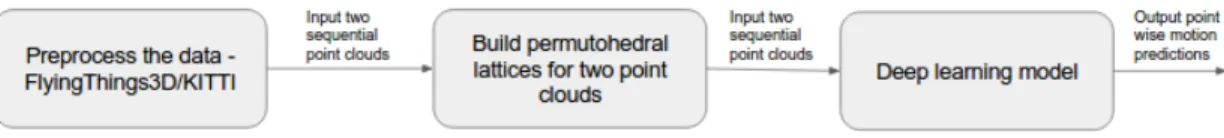
In deep learning, pre-processing the dataset is perhaps a more critical step than performing convolutions. It is important to have a dataset that generalizes well for the task. Hence section 3.5 and section 3.6 provide detailed information about how the two datasets are processed for training. It is also important to choose a metric for an informative evaluation of the performance of the model. We have chosen the F1 score to evaluate our motion segmentation approach. It is a combination of the precision and recall metrics of the network predictions and this makes us believe it is a strong evaluation metric. We train our model on a GeForce RTX2080 11GB GPU. It is to be noted that the training will have different memory requirements for different training samples. So it is common to see GPU usage fluctuations while training. This behavior can be attributed to the fact that each lattice generated for a point cloud will be different in shape and will have different memory requirements to run convolutions on it. Figure 3.1 gives an overview of the major processes discussed in this chapter and the system flow.

(33)

3.2 Point Cloud Representation

Numerous popular representations of point cloud data exist. Some of them are based on the regular grid and a spherical image. Many point cloud processing networks can only operate on a fixed number of input points. Unlike these networks, the permutohedral lattice based network as introduced in [15] is not constrained by the number of input points and is very flexible with respect to the size of the point cloud. Unlike many conventional point cloud processing methods, the permutohedral lattice does not process points in clusters. It also does not need prior filtering approaches to reduce the point cloud size. Many applications filter the input point cloud by using filters like Approximate Voxel Filter to reduce the size of the point cloud, in turn reducing the computation. Permutohedral lattices can be used to represent the point cloud as a whole.

Upon introduction, permutohedral lattices were predominantly used for high dimensional Gaussian filtering [1, 20]. Bilateral filters and non-local means were the major filters tested. [20] discussed a beautiful idea of the use of permutohedral lattice as a representation of independent image features like color values. These lattices can be used to represent a multi-dimensional feature space i.e its vertices can be a representation of the 3D location of the point along with the point’s inten-sity value. In fact, when compared [1] with Gaussian K-D tree and bilateral grid, permutohedral lattice proved to be the fastest method for dimensionalities from 5 to 20, subject to the filter sizes. Because of the efficiency of this lattice in handling high dimensions easily, it becomes an attractive choice for multi-dimensional convo-lutions. Permutohedral lattices are also very accommodating towards sparse input data. The LiDAR data is inherently sparse. The data structure generously allows a cost-effective representation of sparse data. In the network layers, only the occupied

(34)

vertices are chosen to scale down the lattices in the downsampling process.

Let us get started with understanding the permutohedral lattice data structure. A permutohedral lattice in the d-dimensional space is actually the projection of a scaled regular grid from the (d+1) dimension. The (d+ 1)_Zd+1 _{scaled regular grid is} a grid in integer coordinate frame ofd+1 dimensions. The vectors in this space need d+ 1 independent variables for their representation. This regular grid is projected along its orthogonal vector~1= [1,1, ...1], on the hyperplane which is defined by the equation 3.1.

~

x·~1= 0 (3.1)

This projection is the permutohedral lattice. The~xis a vector on the hyperplane. Since~1is a normal to this plane, the dot product of these two vectors is always zero. This hyperplane is a subspace of_Rd+1_{. This means that the hyperplane contains the} null space of_Rd+1_{and it follows the properties of closure under addition and closure} under scalar multiplication. The sum of any two vectors chosen from the hyperplane should also lie on the hyperplane. Also, when a vector chosen from the hyperplane is multiplied with a scalar from _Rd+1, the result should lie on the hyperplane. This hyperplane is embedded in the_Rd+1 space. The lattice is spanned by the projections of the standard basis of the (d+ 1)_Zd+1 _{space onto the hyperplane.}

The permutohedral lattice consists of uniform simplices with integer coordinates for the vertices. All the vertices of this lattice have a consistent remainder when divided by d+ 1. This helps to shed light on another major property of the per-mutohedral lattice - the coordinates of the lattice are such that the sum of all these coordinates is always zero. A short example of a permutohedral lattice as explained in [1] is given using Figure 3.2.

(35)

Figure 3.2: A 2-dimensional permutohedral lattice [1]

bedded in the 3-dimensional space. This hyperplane passes through the origin of the 3-dimensional space. When we get the LiDAR point cloud in this 3-dimensional space, which is normally the case, we can easily project every point onto this lattice and find its enclosing simplex. This point is then interpolated to the vertices of the simplex using barycentric interpolations. The interpolations will be explained in detail in the section 3.3.

The major advantage of using the permutohedral lattice is its time complexity and space complexity for filtering operations. The vertices of the enclosing simplex of every point and its barycentric weights can be found in O(d2_{) time. For}_n _points, the time complexity becomes O(nd2_{). The space complexity for performing filtering} operations on the lattice is O(nd). Both the time complexity and space complexity are relatively less for high d value when compared with other representations and this makes the lattice more attractive.

(36)

3.3 Convolutional Neural Network

This section gives critical information about the network we used for training and evaluating the motion segmentation pipeline. This network is derived from the network proposed in [15]. [15] proposes two networks for scene flow estimation - a deep network and a shallow network. We modify the shallow network and present competitive results for the motion segmentation task.

Motion segmentation is a task that benefits from temporal information. Hence we input a sequence of two point clouds as input to the network. The network is built in such a way that the output is the point-wise predictions for the points from the first point cloud. The predictions are for binary labels- a point can bemovingor non-moving. Since we deal with point cloud data which is 3-dimensional, the network and convolutions are different from the trivial image-based convolutions. Bilateral Convolutional Layers [18,20] are the primitives of the network. The network follows aSplat-Conv-Slice methodology using these layers. The following points give a basic understanding of this three-step methodology.

• Splat: The Splat step refers to the interpolation of the incoming points on the vertices of the permutohedral lattice. It is important to interpolate these points in the continuous space onto a discrete space so that we can easily run convolutions on this lattice. This step can be visualized in Figure 3.3a. • Conv: This is the convolution step. In this step, a sparse convolution is

performed on the lattice points which are occupied. A hash map is maintained to record the occupied positions of the sparse lattice. These occupied vertices are then included in the scaled-down lattice in the encoding layers.

(37)

(a) Splatting step (b) Slicing step

Figure 3.3: In (a), the red input point interpolates to the yellow vertices of the enclosing simplex and in (b), interpolations are performed to get back the original input point

to their original positions as in the input point cloud. This can be visualized in Figure 3.3b.

The Splat, Conv, and Slice steps together can be easily visualized in Figure 3.4. The trivial method is to compute all the steps of the Splat-Conv-Slice methodology in each BCL layer. But a more efficient way is to device new layers which do only part of the computation. The proposed network as implemented by [15] uses such layers which are named - DownBCL and UpBCL. The DownBCL layers are for downsampling the points and the UpBCL layers are for upsampling of the points. The specialty of these layers is that the DownBCL layers only perform Splat and Conv operations whereas the UpBCL layers only perform Conv and Slice operations. The DownBCL layers are stacked and the occupied vertices in the lattice become the input for the scaled-down lattice in the next layer. This process downsamples the points and eventually helps in building a fine-to-coarse feature map. The UpBCL layers use skip connections from the DownBCL layers to upsample the points and finally interpolate them back to their original position as per the first point cloud. This part-wise computation in separate layers helps in reducing the computation

(38)

time and provides an opportunity to explore a much deeper network.

Figure 3.4: Splat-Conv-Slice steps for BCL layers using a permutohedral lattice [15]

The interpolations in theSplat andSlice step are done using Barycentric interpo-lations. This method interpolates a continuous point to the vertices of its enclosing simplex using weights and vice versa. These interpolation weights are the same for the splatting and slicing operation for a point. As explained in [15], if i is a point from the point cloud which needs to be interpolated, let D(i) be the vertices of the simplex in which this point is projected in the permutohedral lattice. Also, for every lattice vertex j, let V(j) be the set of input points that lie in the simplex with this point as the vertex. If bij is the barycentric weight for splatting the input point to

the lattice vertex j, then the BCL operations for the point i can be represented as given in equation 3.2. v0_i = X j∈D(i) bij ·g( X k∈V(j) bkj ·vk) (3.2)

In the above equation,v_i0 is the filtered signal value(position vector in the lattice

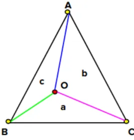
space) and g(·) represents the convolution. The weights for barycentric interpola-tions are usually calculated using simple geometry. The idea of barycentric interpo-lations can be understood as follows. If we consider a simplex as shown in Figure 3.5, a is the weight to interpolate the point to vertex A, b is the weight for inter-polating the point to the vertex B and c is the weight to interpolate it to C. The

(39)

weights are usually calculated using the ratio of areas of sub-simplex to the area of the whole simplex.

Figure 3.5: Barycentric interpolation

The weightsa,b, and ccan be calculated as given in the following equations.

a=ar(∆OBC)/ar(∆ABC) (3.3)

b =ar(∆AOC)/ar(∆ABC) (3.4)

c=ar(∆AOB)/ar(∆ABC) (3.5)

Since the input point clouds are unstructured and sparse, it is helpful to nor-malize the inputs to the lattice. A density normalization scheme based on the barycentric weights is employed in the network while splatting. For a vertex of the lattice, the normalization is done by dividing by the sum of weights for points inter-polating to that vertex. The normalized signal uj will look as shown in the equation

(40)

3.6. uj = P k∈V(j)bkj·vk P k∈V(j)bkj (3.6) Another important layer in this network is the CorrBCL layer. This layer is perhaps the most crucial and unique layer of the network. The CorrBCL layer takes full advantage of the flexibility of the permutohedral lattice to incorporate point clouds of different sizes. The CorrBCL uses the barycentric interpolation scheme to use just one permutohedral lattice to represent both the incoming point clouds. The operations in the CorrBCL layer are executed using Patch correlation and Displacement filtering.

Since we are dealing with two point clouds that differ spatially and temporally, it is important to fuse information from both of them efficiently. ThePatch correlation method proves to be a great method in this regard. Considering a point from each point cloud projected onto the common lattice, their corresponding neighbors are found and concatenated. In simple terms, the patches for both points are concate-nated. A convolution operation is run on such concatenations. Furthermore, points in the first point cloud are offset to local neighborhood points and matched with the signals from the second point cloud present there. An aggregating convolution is used to fuse this information. This process is named Displacement filtering.

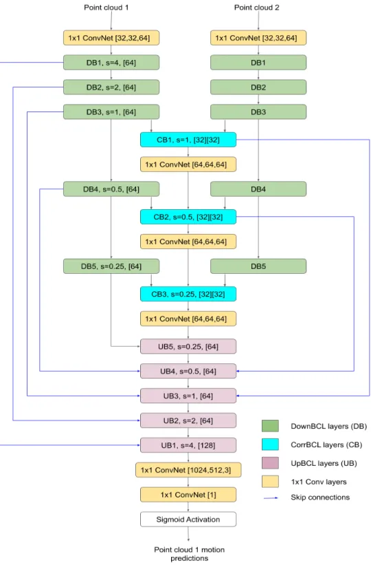
The network architecture is shown in Figure 3.6. The architecture uses three CorrBCL layers. The output from each CorrBCL layer is concatenated with the signals from the first point cloud to input into the next CorrBCL layer. The inputs from the second point cloud are handled individually. A leaky ReLU activation is used throughout the model except for the last two layers. The last layer is activated using the sigmoid function to receive probabilities of predictions. While training, we

(41)

from the first and second point cloud and project them onto the lattice. We use the Adam optimizer for Stochastic Gradient Descent.

3.4 Loss Functions

Supervised learning algorithms require a loss function for finding the error between the prediction and the ground truth for every training sample. In simple words, the loss function generates a heavy penalty if the prediction is very different as compared to the ground truth. A large error indicates that the network has not yet learned to understand the feature embeddings of the dataset. The error ideally should reduce as the training progresses. There are many loss functions to choose from and the choice of the loss function depends on a lot of parameters. The choice of the loss will depend on factors like the task at hand(regression or classification), the class imbalance in the dataset, the number of outliers in the dataset, the type of learning algorithm chosen, etc. There is no single loss function that suits all purposes. The same loss function may not even work well for the same operation on different datasets. Here, we discuss three major loss functions which helped us in training for motion segmentation. Since ours is a binary classification task, the loss functions which we relied upon were binary cross entropy(BCE) loss, focal loss, and soft F1 loss. We chose to experiment on these loss functions because these loss functions are popular for binary classification. Also, the attractive feature of the focal loss is that it offers hyperparameters that can be tuned. The soft F1 loss tries to optimize the F1 score and that is a great advantage.

(42)

Figure 3.6: Network architecture for motion segmentation. The values in brackets are the number of output channels of the layers. Two values in the CorrBCL layers correspond to Patch correlation and Displacement filtering.

(43)

3.4.1 Binary Cross Entropy Loss

In the motion segmentation task, we want to predict if a point is moving or not. Hence we just have two labels in the ground truth - moving, non-moving. The sigmoid activation in the last layer of the network gives out the result in the range of 0 to 1. This output is the probability of a point to be moving. A probability tending to 1 indicates that the network is confident that the point is moving. Whereas if the probability tends to 0, the network is confident that the point is non-moving. The binary cross entropy loss is a log loss that helps in calculating the confidence of the network in predicting the motion state of every training sample. If the ground truth and the prediction deviate by a large value, then the loss function should give a large error and vice versa. The loss can be calculated as shown in equation 3.7.

Ebceloss= −1 N N X i=1

yi·log(p(yi)) + (1−yi)·log(1−p(yi)) (3.7)

In the equation 3.7,yi is the ground truth target value andp(yi) is the probability

predicted by the network. It can be easily noticed that when the target value is 1 i.e the point is actually moving, BCE loss adds the log(p(yi)) term to the overall loss.

When the target value is 0 (non-moving point), the function adds log(1−p(yi)) to

the loss. So the loss of every training sample would be

Ebcelossi =      log(p(yi)), yi = 1 log(1−p(yi)), yi = 0 (3.8)

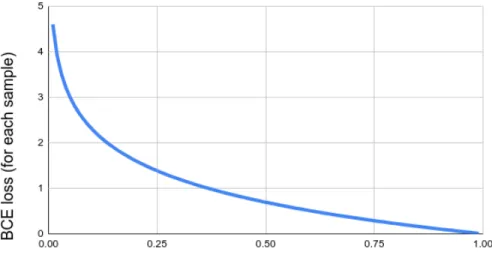
The loss is averaged over all the points from the point cloud. The function calculates the negative log loss because the log provides negative values when the inputs are in the range 0 to 1. Also, another reason for choosing log values in this loss function is that the loss increases exponentially when the predictions are near

(44)

0 and the target value is 1. Since the objective of the network is to reduce the loss, this heavy loss will motivate the network to provide better predictions. This can visually be understood from the log loss graph in Figure 3.7.

Figure 3.7: Log loss graph when the ground truth is 1

3.4.2 Focal Loss

Focal loss is a popular loss function used particularly with datasets that might have unbalanced class sizes. This loss was introduced in [23] to perform dense object detection. This loss builds upon the BCE loss. This loss gives more emphasis on the hard training samples. It heavily penalizes the samples which are hard to classify(the under-sampled class) than the easily classified training samples(the dominant class). For example, if the network is supposed to do a foreground-background classification, and if the background class occupies most of the scene, then background class will dominate the training samples and it will be easy for the network to predict this class correctly. However, it is important to classify the foreground with as much precision as the background and the traditional BCE loss will not be a great help

(45)

in this case. [23] used the focal loss for dense object detection. The objective of this paper is to segregate the objects from the background. Since there is a serious class imbalance problem, the BCE loss is reshaped to include a weighting factor. This weighting factor is listed in equation 3.9

w= (1−pt)γ (3.9)

The pt variable in the equation 3.9 is defined as

pt=e−Ebceloss (3.10)

The focal loss in its raw form is modeled as

Ef ocal =w∗Ebceloss (3.11)

This loss is meant to give more importance to training samples which are hard to classify. In our case, we are more worried about classifying the moving points with certainty. If the moving points have the label 1 and the non-moving points as 0, then the weight will have a large value when the moving point is wrongly classified. The weight will be a relatively small value when a non-moving point has been classified as a moving point. This means the loss increases by a large amount when the moving points are classified wrong. Focal loss differentiates easily between the hard and easy samples. Another factor α is usually added to balance the two classes in terms of their quantity. The value of α can be set based on the ratio of imbalance between the two classes or this parameter can be tuned using cross-validation. The focal loss then

(46)

becomes-Ef ocal =α∗w∗Ebceloss (3.12)

It can be visualized from Figure 3.8 that focal loss as given in equation 3.12 is the same as the BCE loss when γ is 0. As γ increases, the value of the focal loss reduces. It can be seen that the focal loss is very small compared to the BCE loss when predictions are closer to 1. This is due to the weighting factor w.

Figure 3.8: Focal loss for different values ofγ when the ground truth is 1

The α and γ are hyperparameters that need to be tuned. [23] has done a study of different combinations of these values and found α = 0.25 and γ = 2 to give the best results for their task. Due to time constraints, we have used these values for our training. This does not mean that these values are best suited to our task. Further analysis is required to choose the best values.

3.4.3 Soft F1 Loss

(47)

overview of the F1 metric and the procedure to calculate this score. To summarize, F1 score is the harmonic mean of the precision and recall measures of the model. The Precision value for a class is the percentage of samples predicted correctly in the total predictions for that class. Meanwhile, recall is the percentage of samples predicted correctly in the total number of samples present in the class(ground truth). Both these measures are equally important to understand the fitness of the model. Hence we use the F1 score which is a combination of both these metrics.

However, it is not trivial to use F1 score into the loss function and the reason for that is the F1 score is not differentiable. Since it is not differentiable, we cannot backpropagate it and update the weights of the network after each batch. A method to make this metric differentiable is introduced in [28]. This article proposes direct embedding of the modified F1 score into the loss function. In most classifier net-works, a threshold is set to classify a predicted probability from the network into a class. In all the loss functions we have used, the threshold is set at 0.5. If the predic-tion from the network is greater than 0.5, then it is considered to be predicting the moving class which has the label 1. If the predictions are less than the threshold, the network is considered to be predicting the non-moving class. While calculating the F1-score, the predicted probabilities are rounded off to either class labels to calculate the true positives, false positives, and the false negatives. To make the F1 score usable i.e to make it differentiable, we do not round off the predictions but use them as they are. They are directly used as the continuous sum of likelihoods to generate the loss. The following equations tell how the modified true positives, false positives, false negatives, and true negatives are calculated. If y is the target vector with ground truth values and y0 is the vector of predictions without the threshold

applied, then the True Positive(TP), False Positive(FP), False Negative(FN), and True Negative(TN) values can be calculated as follows.

(48)

T P = n X i=1 (y0 ∗y) (3.13) F P = n X i=1 (y0∗(1−y)) (3.14) F N = n X i=1 ((1−y0)∗y) (3.15) T N = n X i=1 ((1−y0)∗(1−y)) (3.16)

Using the above equations, the modified F1 scores of both the binary classes will be calculated as follows. Here we consider the two classes - moving and non-moving.

F1moving = 2∗T P (2∗T P +F N +F P) (3.17) F1non−moving = 2∗T N (2∗T N+F N +F P) (3.18)

It is to be noted that, while programming these equations during training, often a small number is added to the denominator so that in any case, the score values do not become indeterminate. These are the modified F1 scores and we need to maximize these scores. Since most of the optimization problems are minimization problems, we will focus on minimizing the following quantities.

costmoving = 1−F1moving (3.19)

(49)

Minimizing the above costs will naturally maximize the F1 scores. Now, to build the loss function, we need to use both equation 3.19 and 3.24. This becomes necessary because if we just use equation 3.19 as the loss function the network will try to predict all the samples as 1 to minimize this loss. Hence the soft F1 loss function is designed as the average of both the costs. This loss function balances scores for both the classes.

Esof t−F1 =

costmoving+costnon−moving

2 (3.21)

3.5 FlyingThings3D Dataset Preparation

Dataset preparation is a critical and herculean task in machine learning. Data scien-tists often spend most of their time in preparing, analyzing, and cleaning the data. If the quality of the dataset is compromised, any number of efforts in developing efficient machine learning algorithms will be futile.

FlyingThings3D [32] is a synthetic dataset prepared mainly for optical flow, scene flow, and disparity estimation. It consists of a huge collection of stereo image sequences. It provides more than 39000 image pairs, perhaps one of the largest datasets for this purpose. The dataset contains stereo images recorded from a camera moving randomly. The camera captures the scene with random objects moving in random directions. The advantage of this dataset is that it is extremely general i.e the objects in the frames do not belong to any particular category. Also, the number of moving pixels in any frame is not constant. For every frame, the dataset provides optical flow to the next frame, optical flow to the previous frame, disparity values of the current frame, disparity change values to the next frame, disparity change values to the previous frame, and motion boundaries. For our work, we use

(50)

optical flow values, disparity values, and disparity change values. The following are the steps that we follow to reshape the data to our needs.

• We need to convert all the pixels of the image into 3D points. This is done using 3D reconstruction. The camera parameters are obtained from the dataset and the following equations are used to find the [X,Y,Z] 3D coordinates from the [x,y,f] image coordinates. f is the focal length of the camera,B is the baseline, and d denotes the disparity.

Z = f∗B d (3.22) X = x∗Z f (3.23) Y = y∗Z f (3.24)

• Once we have the point cloud from the first pair of left and right images, we use the forward optical flow data and the disparity change values to reconstruct the second point cloud from the first.

• We use the motion segmentation labels provided by [42] for the first point cloud in every pair.

It is to be noted that even though we have correspondences between both the point clouds as mentioned in the above process, we do not use this information. While training, random points are chosen from the first point cloud and separately from the second point cloud to form the lattices. Furthermore, only the points which

(51)

uncertainty of depth measurements grow quadratically with the distance. Hence as mentioned in [15], we choose the distance threshold to be 35m.

3.6 KITTI Dataset Preparation

We use the LiDAR dataset open-sourced by [14] for this task. Semantic labels for this dataset are provided in [4]. From these labels, we understand that there are extremely less number of moving points in this dataset. Hence, we modify this dataset to simulate some motion into the dataset. The following are the steps that we follow.

• We get the first 360◦ point cloud from the dataset. We use the ground truth pose information to reconstruct the next 3D point cloud from the first. • We reconstruct the second point cloud from the first to find correspondences

for simulating motion. The correspondence information is not used while training. It is used just to generate the dataset.

• We add a random uniform noise in the range -0.2 to 0.2 to some points in the first point cloud. We then add a fraction of this noise to the corresponding points in the second point cloud. Basically, before adding the noise, we know that the point was a static point. After adding the noise, the point is not where it should have been for it to be static and hence we label this point as moving.

• Adding noise to the point clouds is done in clusters. In the real world, there are usually clusters of points that move together. For example, many points lie on a car and these points move together. We add the same noise to 5 consecutive points.

(52)

(a) MotionI class (b) MotionII class (c) MotionIII class

Figure 3.9: Demonstration of different motion content in point cloud samples. The red points indicate motion and the green points indicate static points

• We make a generalized dataset in terms of the percentage of noise in the point clouds. We randomly add noise to the point clouds such that some point clouds have less than 30% moving points(named as the MotionI class), some have 30-60% of the points moving(named as the MotionII class) and the rest have 60-75% of the points moving(called the MotionIII class). These point clouds are chosen at random for each percentage value. These classes can be visualized in Figure 3.9.

We separate the generalized dataset into three sets. About 20% of data is stored for testing, 20% is stored for validation, and the rest for training(only a fourth of this data is used for training due to time constraints). Even in this dataset, we only choose points that are closer than 35m from the sensor. Also, the advantage of the KITTI dataset is that it is a real LiDAR dataset that has values in the 360◦ angular

range. The sparsity of the LiDAR is also well captured in this dataset.

3.7 Evaluation Criteria

It is important to choose evaluation metrics that give valuable information about how the model has fared. F1 score is the major metric that we observe. We also

Motion Segmentation for Autonomous Robots Using 3D Point Cloud Data

Digital WPI

Digital WPI

Motion Segmentation for Autonomous Robots Using 3D Point

Motion Segmentation for Autonomous Robots Using 3D Point

Cloud Data

Cloud Data

Motion Segmentation for Autonomous Robots Using 3D

Point Cloud Data

Contents

List of Figures

List of Tables

Chapter 1

Introduction

1.1

Motivation

1.2

Background

1.2.1

Understanding LiDAR Data

1.2.2

Understanding Motion Segmentation

1.3

Problem Formulation

1.4

Contributions

1.5

Outline Of This Thesis

Chapter 2

Related Work

2.1

Why is Motion Information Important?

2.2

Camera Data for Segmentation

2.3

Point Cloud Data for Segmentation

2.4

Datasets

Chapter 3

Methodology

3.1

System Overview

3.2

Point Cloud Representation

3.3

Convolutional Neural Network

3.4

Loss Functions

3.4.1

Binary Cross Entropy Loss

3.4.2

Focal Loss

3.4.3

Soft F1 Loss

3.5

FlyingThings3D Dataset Preparation

3.6

KITTI Dataset Preparation

3.7

Evaluation Criteria